Stanford CS25: V1 I Decision Transformer: Reinforcement Learning via Sequence Modeling

00:00:00.000 | So I'm excited to talk today about our recent work on using transformers for reinforcement

00:00:12.420 | learning.

00:00:13.420 | And this is joint work with a bunch of really exciting collaborators, most of them at UC

00:00:20.640 | Berkeley, and some of them at Facebook and Google.

00:00:24.480 | I should mention this work was led by two talented undergrads, Li Chen and Kevin Liu.

00:00:31.920 | And I'm excited to present the results we had.

00:00:35.280 | So let's try to motivate why we even care about this problem.

00:00:40.360 | So we have seen in the last three or four years that transformers, since the introduction

00:00:48.080 | in 2017, have taken over lots and lots of different fields of artificial intelligence.

00:00:55.600 | So we saw them having a big impact for language processing.

00:00:59.040 | We saw them being used for vision, using the vision transformer very recently.

00:01:05.540 | They were in nature trying to solve protein folding.

00:01:09.560 | And very soon they might just replace us as computer scientists by having an automatically

00:01:14.080 | generate code.

00:01:16.280 | So with all of these advances, it seems like we are getting closer to having a unified

00:01:21.160 | model for decision-making for artificial intelligence.

00:01:25.880 | But artificial intelligence is much more about not just having perception, but also using

00:01:32.760 | the perception knowledge to make decisions.

00:01:35.120 | And this is what this talk is going to be about.

00:01:38.000 | But before I go into actually thinking about how we will use these models for decision-making,

00:01:44.640 | here is a motivation for why I think it is important to ask this question.

00:01:50.020 | So unlike models for RL, when we look at transformers for perception modalities, like I showed in

00:01:58.280 | the previous slide, we find that these models are very scalable and have very stable training

00:02:05.200 | dynamics.

00:02:06.200 | So you can keep-- as long as you have enough computation and you have more and more data

00:02:11.400 | that can be sourced, you can train bigger and bigger models and you'll see very smooth

00:02:16.640 | reductions in the loss.

00:02:20.240 | And the overall training dynamics are very stable and this makes it very easy for practitioners

00:02:26.880 | and researchers to build these models and learn richer and richer distributions.

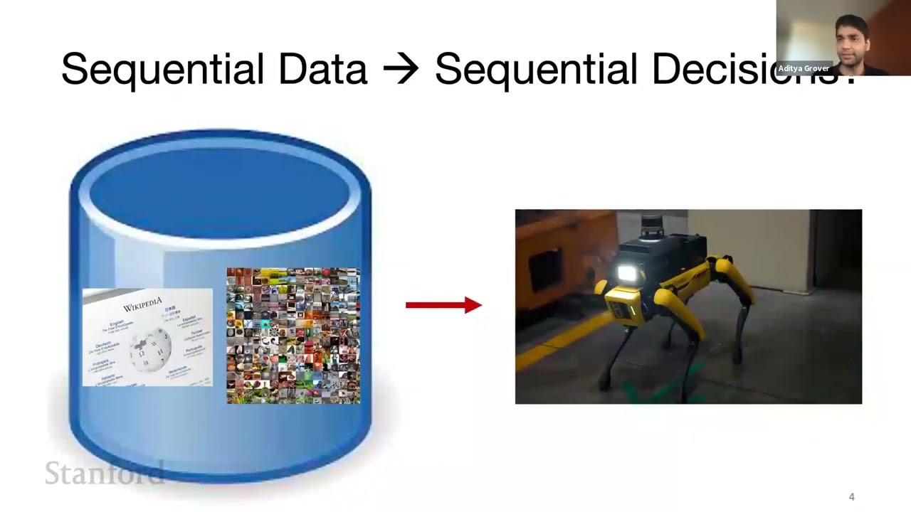
00:02:34.160 | So like I said, all of these advances have so far occurred in perception.

00:02:39.360 | What we'll be interested in this talk is to think about how we can go from perception,

00:02:44.800 | looking at images, looking at text, and all these kinds of sensory signals, to then going

00:02:49.840 | into the field of actually taking actions and making our agents do interesting things

00:02:56.280 | in the world.

00:02:59.800 | And here, throughout the talk, we should be thinking about why this perspective is going

00:03:05.280 | to enable us to do scalable learning, like I showed in the previous slide, as well as

00:03:10.480 | bring stability into the whole procedure.

00:03:13.760 | So sequential decision making is a very broad area.

00:03:17.560 | And what I'm specifically going to be focusing on today is the one route to sequential decision

00:03:23.560 | making, that's reinforcement learning.

00:03:26.460 | So just as a brief background, what is reinforcement learning?

00:03:31.920 | So we are given an agent who is in a current state, and the agent is going to interact

00:03:38.840 | with the environment by taking actions.

00:03:42.960 | And by taking these actions, the environment is going to return to it a reward for how

00:03:49.160 | good that action was, as well as the next state into which the agent will transition,

00:03:54.680 | and this whole feedback loop will continue on.

00:03:58.720 | The goal here for an intelligent agent is to then, using trial and error-- so try out

00:04:05.520 | different actions, see what rewards will lead to-- learn a policy which maps your states

00:04:11.240 | to actions, such that the policy maximizes the agent's cumulative rewards over time horizon.

00:04:17.760 | So you take a sequence of actions, and then based on the reward you accumulate for that

00:04:22.560 | sequence of actions, we'll judge how good your policy is.

00:04:27.960 | This talk is also going to be specifically focused on a form of reinforcement learning

00:04:33.800 | that goes by the name of offline reinforcement learning.

00:04:37.520 | So the idea here is that what changes from the previous picture where I was talking about

00:04:43.040 | online reinforcement learning is that here, now instead of doing actively interacting

00:04:50.080 | with the environment, you have a collection of log data of interactions.

00:04:55.740 | So think about some robot that's going out in the fields, and it collects a bunch of

00:05:00.240 | sensory data, and you've all logged it.

00:05:02.960 | And using that log data, you now want to train another agent-- it could be another robot--

00:05:09.200 | to then learn something interesting about that environment just by looking at the log

00:05:14.400 | data.

00:05:15.400 | So there's no trial and error component, which is currently one of the extensions of this

00:05:24.380 | framework, which will be very exciting.

00:05:26.520 | So I'll talk about this towards the end of the talk, why it's exciting to think about

00:05:30.400 | how we can extend this framework to include an exploration component and have trial and

00:05:36.000 | error.

00:05:37.000 | OK, so now to go more concretely into what the motivating challenge of this talk was

00:05:44.240 | now that we have introduced RL.

00:05:47.140 | So let's look at some statistics.

00:05:50.200 | So large language models have billions of parameters.

00:05:55.380 | And today, they have roughly about 100 layers and transformer.

00:06:01.600 | They're very stable to train using supervised learning style losses, which are the building

00:06:07.940 | blocks of autoregressive generation, for instance, or for mass language modeling, as in BERT.

00:06:15.920 | And this is like a field that's growing every day.

00:06:20.280 | And there's a course at Stanford that we're all taking just because it has had such a

00:06:24.640 | monumental impact on AI.

00:06:27.240 | RL policies, on the other hand-- and I'm talking about deep RL-- the maximum they would extend

00:06:35.920 | to is maybe millions of parameters or 20 layers.

00:06:42.080 | And what's really unnerving is that they're very unstable to train.

00:06:46.200 | So the current algorithms for reinforcement learning, they're built on a mostly dynamic

00:06:51.960 | programming, which involves solving an inner loop optimization problem that's very unstable.

00:06:57.280 | And it's very common to see practitioners in RL looking at reward codes that look like

00:07:02.920 | this.

00:07:03.960 | So what I really want you to see here is the variance in the returns that we tend to get

00:07:09.720 | in RL.

00:07:11.120 | It's really huge, even after doing multiple rounds of experimentation.

00:07:15.660 | And that is really at the core got to done with the fact that our algorithms, our learning

00:07:22.960 | objectives, need better improvements so that the performance can be stably achieved by

00:07:28.840 | agents in complex environments.

00:07:33.440 | So what this work is hoping to do is it's going to introduce transformers.

00:07:41.440 | And I'll first show in one slide what exactly that model looks like.

00:07:45.640 | And then we're going to go into deeper details of each of the components.

00:07:49.920 | I have a--

00:07:50.920 | Quick question.

00:07:51.920 | Yeah, can I ask a question real quick?

00:07:52.920 | Yes.

00:07:53.920 | And--

00:07:54.920 | Thank you.

00:07:55.920 | [INAUDIBLE]

00:07:56.920 | What I'm curious to know is, what is the cause for why RL typically has several orders

00:08:05.720 | of magnitude fewer parameters?

00:08:07.440 | That's a great question.

00:08:11.000 | So typically, when you think about reinforcement learning algorithms, in deep RL in particular,

00:08:18.560 | so the most common algorithms, for example, have different networks playing different

00:08:25.000 | roles in the task.

00:08:29.200 | So you have a network, for instance, playing the role of an actor, so it's trying to figure

00:08:34.400 | out a policy.

00:08:35.400 | And then there'll be a different network that's playing the role of a critic.

00:08:39.600 | And these networks are trained on data that's adaptively gathered.

00:08:45.340 | So unlike perception, where you will have a huge data set of interactions on which you

00:08:51.760 | can train your models, in this case, the architectures and even the environments, to some extent,

00:09:00.160 | are very simplistic because of the fact that we are trying to train very small components,

00:09:07.240 | the functions that we are training, and then bringing them all together.

00:09:11.200 | And these functions are often trained in not super complex environments.

00:09:17.760 | So it's a mix of different issues.

00:09:20.020 | I wouldn't say it's purely just about the fact that the learning objectives are at fault,

00:09:26.720 | but it's a combination of the environments we use, the combination of the targets that

00:09:31.200 | each of the neural networks are predicting, which leads to networks which are much bigger

00:09:37.560 | than what we currently see, tending to overfit.

00:09:41.920 | And that's why it's very common to see neural networks with much fewer layers being used

00:09:47.640 | in RL as opposed to perception.

00:09:50.640 | Thank you.

00:09:52.480 | Do you want to ask a question?

00:09:58.200 | Yeah.

00:09:59.200 | Yeah, I was going to.

00:10:00.200 | Is there a reason why you chose offline RL versus online RL?

00:10:06.440 | That's another great question.

00:10:07.680 | So the question is, why offline RL as opposed to online RL?

00:10:12.080 | And the plain reason is because this is the first work trying to look at reinforcement

00:10:17.120 | learning.

00:10:18.120 | So offline RL avoids this problem of exploration.

00:10:23.640 | You are given a log data set of interactions.

00:10:25.800 | You're not allowed to further interact with the environment.

00:10:29.400 | So just from this data set, you're trying to unearth a policy of what the optimal agent

00:10:35.080 | would look like.

00:10:36.620 | So it would.

00:10:37.620 | Right.

00:10:38.620 | If you do online RL, wouldn't that just give you this opportunity of exploration, basically?

00:10:44.840 | It would.

00:10:45.840 | It would.

00:10:46.840 | And what it would also do, which is technically challenging here, is that the exploration

00:10:53.000 | would be harder to encode.

00:10:54.800 | So offline RL is the first step.

00:10:56.480 | There's no reason why we should not study why online RL cannot be done.

00:11:00.960 | It's just that it provides a more contained setup where ideas from transformers will directly

00:11:06.920 | extend.

00:11:07.920 | Okay.

00:11:08.920 | Sounds good.

00:11:09.920 | So let's look at the model and it's really simple on purpose.

00:11:19.480 | So what we're going to do is we're going to look at our offline data, which is essentially

00:11:24.860 | in the form of trajectories.

00:11:27.140 | So offline data would look like a sequence of states, actions, returns over multiple

00:11:34.200 | time steps.

00:11:35.200 | It's a sequence.

00:11:37.420 | So it's natural to think of us as directly feeding as input to a transformer.

00:11:44.100 | In this case, we use a causal transformer as it's common in GPT.

00:11:50.160 | So we go from left to right.

00:11:51.820 | And because this dataset comes with the notion of time step, causality here is much more

00:11:57.400 | well-intended than the general meaning that's used for perception.

00:12:01.640 | This is really causality, how it should be in perspective of time.

00:12:07.200 | What we predict out of this transformer are the actions conditioned on everything that

00:12:14.240 | comes before that token in the sequence.

00:12:17.840 | So if you want to predict the action at this T minus one step, we'll use everything that

00:12:22.480 | came at time step T minus two, as well as the returns and states at time step T minus

00:12:31.160 | one.

00:12:34.400 | So we will go into the details of how exactly each of these are encoded.

00:12:41.320 | But essentially, this is in a one liner.

00:12:45.320 | It's taking the trajectory data from the offline data, treating it as a sequence of tokens,

00:12:50.400 | passing it through a causal transformer, and getting a sequence of actions as the output.

00:12:56.280 | OK, so how exactly do we do the forward pass through the network?

00:13:03.720 | So one important aspect of this work, which is we use states, actions, and this quantity

00:13:12.440 | called returns to go.

00:13:14.880 | So these are not direct rewards.

00:13:16.400 | These are returns to go, and let's see what they really mean.

00:13:22.880 | So this is our trajectory that goes as input.

00:13:28.160 | And the returns to go are the sum of rewards starting from the current time step until

00:13:35.840 | the end of the episode.

00:13:38.080 | So really what we want the transformer is to get better at using a target return-- this

00:13:45.760 | is how you should think of returns to go-- as the input in deciding what action to take.

00:13:52.880 | This perspective is going to have multiple advantages.

00:13:55.040 | It will allow us to actually do much more than offline RL and generalizing to different

00:14:00.000 | tasks by just changing the returns to go.

00:14:04.520 | And here it's very important.

00:14:06.360 | So at time step one, we will just have the overall sum of rewards for the entire trajectory.

00:14:12.840 | At time step two, we subtract the reward we get by taking the first action, and then have

00:14:18.600 | the sum of rewards for the remainder of the trajectory.

00:14:22.720 | OK, so that's how we call it returns to go, like how many more rewards in accumulation

00:14:30.360 | you need to acquire to fulfill your return goal that you set in the beginning.

00:14:39.240 | What is the output?

00:14:40.600 | The output is the sequence of predicted actions.

00:14:44.440 | So as I showed in the previous slide, we use a causal transformer.

00:14:49.040 | So we'll predict in sequence the desired actions.

00:14:55.320 | The attention, which is going to be computed inside the transformer, will take in an important

00:15:03.680 | hyperparameter k, which is the context length.

00:15:06.680 | We see that in perception as well here.

00:15:09.480 | And for the rest of the talk, I'm going to use the notation k to denote how many tokens

00:15:14.000 | in the past would we be attending over to predict the action and the current time step.

00:15:21.680 | OK, so again, digging a little bit deeper into code, there are some subtle differences

00:15:29.680 | with how a decision transformer operates as opposed to a normal transformer.

00:15:37.920 | The first is that here, the time step notion is going to have a much bigger semantics that

00:15:46.880 | extends across three tokens.

00:15:50.400 | So in perception, you just think about the time step per word, for instance, like an

00:15:57.040 | NLP or per patch for vision.

00:15:59.880 | And in this case, we will have a time step encapsulating three tokens, one for the states,

00:16:05.680 | one for the actions, and one for the rewards.

00:16:09.120 | And then we'll embed each of these tokens and then add the position embedding as is

00:16:15.200 | common in a transformer.

00:16:18.040 | And we feed those inputs to the transformer.

00:16:23.000 | At the output, we only care about one of these three tokens in this default setup.

00:16:27.920 | I will show experiments where even the other tokens might be of interest as target predictions.

00:16:33.360 | But for now, let's keep it simple.

00:16:34.800 | We want to learn a policy, a policy that's trying to predict actions.

00:16:38.840 | So when we try to decode, we'll only be looking at the actions from the hidden representation

00:16:46.160 | in the pre-final layer.

00:16:47.640 | OK, so this is the forward pass.

00:16:49.920 | Now, what do we do with this network?

00:16:51.720 | We train it.

00:16:52.720 | How do we train it?

00:16:53.720 | Sorry, just a quick question on semantics there.

00:16:57.760 | If you go back one slide, the plus in this case, the syntax means that you are actually

00:17:03.040 | adding the values element-wise and not concatenating them.

00:17:05.440 | Is that right?

00:17:06.440 | That is correct.

00:17:07.440 | OK, cool.

00:17:08.440 | So let me check.

00:17:09.440 | Thanks.

00:17:10.440 | OK, so what's the last function?

00:17:11.440 | Follow up on that.

00:17:12.440 | I thought it was concatenated.

00:17:13.440 | Why are we just adding it?

00:17:14.440 | Sorry.

00:17:15.440 | Can you go back?

00:17:16.440 | Yeah, I think it's a design choice.

00:17:17.440 | You can concatenate.

00:17:18.440 | You can add it.

00:17:19.440 | It leads to different functions being encoded.

00:17:20.440 | In our case, it was addition.

00:17:34.760 | OK, why did you-- did you try the other one and it just didn't work, or why is that?

00:17:42.920 | Because I think intuitively, concatenating would make more sense.

00:17:48.880 | So I think both of them have different use cases for the functional encoding.

00:17:55.520 | One is really mixing in the embeddings for the state and basically shifting it.

00:18:01.760 | So when you add something, if you think of the embedding of the states as a vector, and

00:18:09.400 | you add something, you are actually shifting it, whereas in the concatenation case, you

00:18:15.080 | are actually increasing the dimensionality of the space.

00:18:20.640 | So those are different choices, which are doing very different things.

00:18:25.680 | We found this one to work better.

00:18:27.960 | I'm not sure I remember if the results were very significantly different if you would

00:18:32.880 | concatenate them, but this is the one which we operate with.

00:18:37.560 | But wouldn't there-- because if you're shifting it, if you have an embedding for a state,

00:18:41.440 | let's say you perform certain actions and you end up at the same state again, you would

00:18:47.120 | want these embeddings to be the same, however, now you're at a different time step.

00:18:51.480 | So you shifted it.

00:18:52.960 | So wouldn't that be harder to learn?

00:18:55.960 | So there's a bigger and interesting question in that what you said is basically, are we

00:19:01.640 | losing the Markov property?

00:19:04.800 | Because as you said, if you come back to the same state at a different time step, shouldn't

00:19:11.400 | we be doing similar operations?

00:19:15.680 | And the answer here is yes, we are actually being non-Markov.

00:19:20.080 | And this might seem very non-intuitive at first, that why is non-Markovness important

00:19:28.080 | here?

00:19:30.080 | And I want to refer to another paper which came very much in conjunction with this, the

00:19:35.640 | triarchy transformer, that actually shows in more detail.

00:19:38.680 | And it basically says that if you were trying to predict the transition dynamics, then you

00:19:43.480 | could have actually had a Markovian system built in here, which would do just as good.

00:19:50.520 | However, for the perspective of trying to actually predict actions, it does have to

00:19:58.440 | look at the previous time steps, even more so when you have missing observations.

00:20:03.200 | So for instance, if you have the observations being a substrate of the true state.

00:20:09.440 | So looking at the previous states and actions helps you better fill in the missing pieces

00:20:16.640 | in some sense.

00:20:17.640 | So this is commonly known as partial observability, where by looking at the previous tokens, you

00:20:22.840 | can do a better job at predicting the actions that you should take at the current time step.

00:20:31.320 | So non-Markovness is on purpose.

00:20:35.280 | And it's not intuitive, but I think it's one of the things that separates this framework

00:20:41.760 | from existing ones.

00:20:44.680 | So it will basically help you-- because RL usually works better on infinite horizon problems,

00:20:51.400 | right?

00:20:52.400 | So technically, the way you formulate it, it would work better on finite horizon problems,

00:20:56.040 | I'm assuming.

00:20:57.040 | Because you want to take different actions based on the history, based on given a fact

00:21:00.800 | that now you're at a different time step.

00:21:03.040 | Yeah.

00:21:04.040 | Yeah.

00:21:05.040 | So if you wanted to work on infinite horizon, maybe something like discounting would work

00:21:10.280 | just as well to get that effect.

00:21:12.680 | In this case, we were using a discount factor of 1, or basically no discounting at all.

00:21:19.960 | But you're right.

00:21:20.960 | If I think we really want to extend it to infinite horizon, we would need to change

00:21:24.400 | the discount factor.

00:21:25.400 | All right.

00:21:26.400 | Thanks.

00:21:27.400 | OK.

00:21:31.680 | So--

00:21:32.680 | Quick question.

00:21:33.680 | Oh.

00:21:34.680 | I think it was just answered in chat, but I'll ask it anyways.

00:21:38.120 | I think I might have missed this, or maybe you're about to talk about it.

00:21:40.760 | The offline data that was collected, what policy was used to collect it?

00:21:44.600 | So this is a very important question, and it will be something I mentioned in the experiment.

00:21:52.640 | So we were using the benchmarks that exist for offline RL, where essentially the way

00:21:58.560 | these benchmarks are constructed is you train an agent using online RL, and then you look

00:22:03.840 | at its replay buffer at some time step while it's training.

00:22:08.960 | So while it's like a medium sort of expert, you collect the transitions it's experienced

00:22:15.420 | so far and make that as the offline data.

00:22:18.240 | It's something which is-- like our framework is very agnostic to what offline data that

00:22:23.560 | you use.

00:22:24.560 | So I've not discussed it so far.

00:22:27.680 | But it's something that in our experiments is based on traditional benchmarks.

00:22:32.000 | Got it.

00:22:33.000 | So the reason I ask isn't-- I'm sure that your framework can accommodate any offline

00:22:37.200 | data.

00:22:38.200 | But it seems to me like the results that you're about to present are going to be heavily contingent

00:22:41.840 | on what that data collection policy is.

00:22:45.240 | Indeed.

00:22:46.240 | Indeed.

00:22:47.240 | And also-- so we will-- I think I have a slide where we show an experiment where the

00:22:53.720 | amount of data can make a difference in how we compare with baselines.

00:22:58.760 | And essentially, we will see how this [INAUDIBLE] especially shines when there is small amounts

00:23:06.060 | of offline data.

00:23:07.060 | OK.

00:23:08.060 | Cool.

00:23:09.060 | Thank you.

00:23:10.060 | OK.

00:23:11.060 | Great questions.

00:23:12.060 | So let's go ahead.

00:23:14.320 | So we have defined our model, which is going to look at these trajectories.

00:23:21.200 | And now, let's see how we train it.

00:23:23.720 | So very simple, we are trying to predict actions.

00:23:27.520 | We'll try to match them to the ones we have in our data set.

00:23:30.840 | If they are continuous, using the mean squared error.

00:23:33.160 | If they are discrete, then we can use the cross-entropy.

00:23:38.320 | But there is something very deep in here for our research, which is that these objectives

00:23:45.760 | are very stable to train and easy to regularize because they've been developed for supervised

00:23:50.520 | learning.

00:23:52.360 | In contrast, what RL is more used to is dynamic programming style objectives, which are based

00:23:57.640 | on the Bellman equation.

00:24:00.040 | And those end up being much harder to optimize and scale.

00:24:05.160 | And that's why you see a lot of the variance in the results as well.

00:24:09.920 | OK.

00:24:11.540 | So this is how we train the model.

00:24:13.280 | Now, how do we use the model?

00:24:14.920 | And that's the point about trying to do rollout for the model.

00:24:19.800 | So here, again, this is going to be similar to doing an autoregressive generation.

00:24:26.640 | There is an important token here, which was the returns to go.

00:24:30.840 | And what we need to set during evaluation, presumably, we want export level performance

00:24:37.640 | because that will have the highest returns.

00:24:41.080 | So we set the initial returns to go, not based on our trajectory, because now we don't have

00:24:47.280 | a trajectory.

00:24:48.280 | We're going to generate a trajectory.

00:24:49.280 | So this is at entrance time.

00:24:51.080 | So we'll set it to the export return, for instance.

00:24:54.800 | So in code, what this whole procedure would look like is basically you set this returns

00:24:59.560 | to go token to have some target return.

00:25:03.800 | And you set your initial state to run from the environment distribution of initial states.

00:25:12.240 | And then you just roll out your decision transformer.

00:25:16.100 | So you get a new action.

00:25:18.840 | This action will also give you a state and reward from the environment.

00:25:23.400 | You append them to your sequence, and you get a new returns to go.

00:25:29.760 | And you take just the context and key, because that's what's used by the transformer to making

00:25:33.920 | predictions, and then feed it back to the decision transformer.

00:25:38.480 | So it's regular autoregressive generation, but the only key point to notice is how you

00:25:44.600 | initialize the transformer for RL.

00:25:49.000 | Sorry, I had one question here.

00:25:52.920 | How much does the choice of the export target return matter?

00:25:55.840 | Does it have to be the mean export reward, or can it be the maximum reward possible in

00:25:59.280 | the environment?

00:26:00.280 | Does the choice of the number really matter?

00:26:04.480 | That's a very good question.

00:26:05.640 | So we generally would set it to be slightly higher than the max return in the data set.

00:26:16.040 | So I think the factor we use is 1.1 times.

00:26:20.280 | But I think we have done a lot of experimentation in the range, and it's fairly robust to what

00:26:29.880 | choice you use.

00:26:31.080 | So for example, for Hopper, export returns about 3,600, and we have found very stable

00:26:36.760 | performance all the way from 3,500, 3,400 to even going to very high numbers, like 5,000,

00:26:46.340 | it works.

00:26:48.520 | Yeah.

00:26:51.000 | So however, I would want to point out that this is something which is not typically needed

00:26:58.240 | in regular RL, like knowing the export return.

00:27:02.560 | Here we are actually going beyond regular RL in that we can choose a return we want,

00:27:07.000 | so we also actually need this information about what the export return is at test.

00:27:13.720 | Sorry.

00:27:14.720 | There's another--

00:27:15.720 | Yeah.

00:27:16.720 | Yes.

00:27:17.720 | Hi.

00:27:18.720 | So it's just that you cannot be on the regular RL, but I'm curious about do you also restrict

00:27:28.240 | this framework to only offline RL, because if you want to run this kind of framework

00:27:34.520 | in online RL, you'll have to determine the returns to go a priori.

00:27:40.220 | So this kind of framework, I think it's kind of restricted to only offline RL.

00:27:44.600 | Do you think so?

00:27:46.320 | Yes.

00:27:47.320 | And I think asking this question as well earlier, that yes, I think for now, this is the first

00:27:55.320 | book, so we were focusing on offline RL where this information can be gathered from the

00:28:00.920 | offline data set.

00:28:04.700 | It is possible to think about strategies on how you can even get this online.

00:28:10.720 | What you'll need is a curriculum.

00:28:12.080 | So early on during training as we're gathering data, you will set-- when you're doing rollouts,

00:28:18.760 | you will set your expert return to whatever you see in the data set, and then increment

00:28:25.400 | it as and when you start seeing that the transformer can actually exceed that performance.

00:28:31.160 | So you can think of specifying a curriculum from slow to high for what that expert return

00:28:37.440 | could be for which you roll out the decision transformer.

00:28:42.920 | I see.

00:28:43.920 | Cool.

00:28:44.920 | Thank you.

00:28:45.920 | So yeah, this was about the model.

00:28:49.940 | So we discussed how this model is-- what the input to this model are, what the outputs

00:28:57.500 | are, what the loss function is used for training this model, and how do we use this model at

00:29:02.920 | test time.

00:29:05.160 | There is a connection to this framework as being one way to instantiate what is often

00:29:12.680 | known as RLS probabilistic inference.

00:29:15.760 | So we can formulate RL as a graphical model problem where you have the states and actions

00:29:23.920 | being used to determine what the next state is.

00:29:27.520 | And to encode a notion of optimality, typically you would also have these additional auxiliary

00:29:32.320 | variables, O1, O2, and so on and forth, which are implicitly saying that encoding some notion

00:29:39.400 | of reward.

00:29:40.720 | And conditioned on this optimality being true, RL is the task of learning a policy, which

00:29:48.120 | is the mapping from states to actions such that we get optimal behavior.

00:29:56.920 | And if you really squint your eyes, you can see that these optimality variables and decision

00:30:03.440 | transformers are actually being encoded by the returns to go.

00:30:07.600 | So if when we give a value that's high enough at test time during rollouts, like the expert

00:30:13.680 | return, we are essentially saying that conditioned on this being the mathematical quantification

00:30:23.480 | of optimality, roll out your decision transformer to hopefully satisfy this condition.

00:30:34.200 | So yeah, so this was all I want to talk about the model itself.

00:30:38.480 | Can you explain that, please?

00:30:41.200 | What do you mean by optimality variables in the decision transformer?

00:30:44.680 | And how do you mean like return to go?

00:30:46.960 | Right.

00:30:47.960 | So optimality variables, we can think in the most simplest context as, let's just say they

00:30:55.760 | were binary.

00:30:56.880 | So 1 is if you solve the goal, and 0 is if you did not solve the goal.

00:31:03.600 | And what basically in that case, you could also think of your decision transformer as

00:31:12.200 | at test time and we encode the returns to go, we could set it to 1, which would basically

00:31:19.040 | mean that conditioned on optimality-- so optimality here means solving the goal as 1-- generate

00:31:28.760 | me the sequence of actions such that this would be true.

00:31:34.160 | Of course, our learning is not perfect, so it's not guaranteed we'll get that.

00:31:39.720 | But we have trained the transformer in a way to interpret the returns to go as some notion

00:31:45.520 | of optimality.

00:31:49.300 | So if I'm interpreting this correctly, it's roughly like saying, show me what an optimal

00:31:55.920 | sequence of transitions look like, because the model has learned both successful and

00:32:00.920 | unsuccessful transitions.

00:32:02.440 | Exactly.

00:32:03.440 | Exactly.

00:32:04.440 | OK.

00:32:05.440 | And as we've seen some experiments, for the binary case, it's either optimal or non-optimal.

00:32:12.720 | But really, this can be a continuous variable, which it is in our experiments.

00:32:16.720 | So we can also see what happens in between experimentally.

00:32:20.840 | OK, so let's jump into the experiments.

00:32:27.520 | So there are a bunch of experiments, and I've picked out a few which I think are interesting

00:32:33.400 | and give the key results in the paper, but feel free to refer to the paper for an even

00:32:39.240 | more detailed analysis on some of the components of our model.

00:32:46.520 | So first, we can look at how well does it do an offline RL.

00:32:49.880 | So there are benchmarks for the Atari suite of environments and the OpenAI Gym.

00:32:56.800 | And we have another environment, Key2Door, which is especially hard because it contains

00:33:01.680 | sparse rewards and requires you to do credit assignment that I'll talk about later.

00:33:06.340 | But across the board, we see that decision transformer is competitive with the state-of-the-art

00:33:13.600 | model-free offline RL methods.

00:33:15.480 | In this case, this was a version of Q-learning designed for offline RL.

00:33:21.960 | And it can do excellent, especially when there is long-term credit assignment where traditional

00:33:28.280 | methods based on TD learning would fail.

00:33:31.480 | Yeah, so the takeaway here should not be that we should be at the stage where we can just

00:33:37.560 | simply substitute the existing algorithms for the decision transformer.

00:33:42.600 | But this is a very strong evidence in favor that this paradigm which is building on transformers

00:33:49.640 | will permit us to better iterate and improve the models to hopefully surpass the existing

00:33:57.640 | algorithms uniformly.

00:33:59.600 | And there's some early evidence of that in harder environments, which do require long-term

00:34:04.520 | credit assignment.

00:34:05.520 | OK.

00:34:06.520 | Can I ask a question here about the baseline, specifically TD learning?

00:34:12.240 | I'm curious to know, because I know that a lot of TD learning agents are feedforward

00:34:15.640 | networks.

00:34:16.640 | Are these baselines, do they have recurrence?

00:34:19.560 | Yeah, yeah.

00:34:22.280 | So I think the conservative Q-learning baselines here did have recurrence, but I'm not very

00:34:29.040 | sure.

00:34:30.040 | So I can check back on this offline and get back to you on this.

00:34:33.640 | OK.

00:34:34.640 | Thank you.

00:34:35.640 | Also, another quick question.

00:34:36.640 | So just how exactly do you evaluate the decision transformer here in the experiment?

00:34:46.440 | So because you need to supply the returns to go, so do you use the optimal policy to

00:34:54.080 | get what's the optimal rewards and speed that in?

00:34:57.360 | Yes.

00:34:58.360 | So here we basically look at the offline data set that was used for training.

00:35:02.160 | And we said, whatever was the maximum return in the offline data, we set the desired target

00:35:10.400 | return to go as slightly higher than that.

00:35:14.080 | So 1.1 was the coefficient we used.

00:35:17.680 | I see.

00:35:18.680 | So the performance-- sorry, I'm not really well-versed in RLs, but how is the performance

00:35:24.360 | defined here?

00:35:25.360 | It's just like, is it how much reward you get actually from the--

00:35:28.800 | Yes.

00:35:29.800 | Yes.

00:35:30.800 | So you can specify a target return to go, but there's no guarantee that the actual actions

00:35:36.560 | that you take will achieve that return.

00:35:40.120 | So you measure the true environment return based on that.

00:35:45.880 | Yeah.

00:35:46.880 | I see.

00:35:47.880 | But then just curious, so are these performance the percentage you get for how much reward

00:35:55.320 | you recover from the actual environment?

00:35:58.200 | Yeah.

00:35:59.200 | So these are not percentages.

00:36:00.200 | These are some way of normalizing the return so that everything falls between 0 to 100.

00:36:05.520 | Yeah.

00:36:06.520 | Yeah.

00:36:07.520 | I see.

00:36:08.520 | Then I just wonder if you have a rough idea about how much reward actually is recovered

00:36:13.720 | by decision transformers.

00:36:15.600 | Does it say, if you specify, I want to get 50 rewards, does it get 49?

00:36:20.040 | Or is this even better sometimes?

00:36:24.320 | That's an excellent question.

00:36:25.600 | And my next slide.

00:36:26.600 | OK.

00:36:27.600 | I see.

00:36:28.600 | Thanks.

00:36:29.600 | So here we're going to answer precisely this question that we're asked is like, if you

00:36:34.360 | feed in the target return, it could be expert or it could also not be expert.

00:36:39.200 | How well does the model actually do in attaining it?

00:36:42.960 | So the x-axis is what we specify as the target return we want.

00:36:49.840 | And the y-axis is basically how much, how well do we actually get.

00:36:54.960 | For reference, we have this green line, which is the oracle.

00:36:58.640 | Which means whatever you desire, the decision transformer gives it to you.

00:37:03.320 | So this would have been the ideal case.

00:37:05.320 | So it's a diagonal.

00:37:08.040 | We also have, because this is offline RL, we have in orange what was the best trajectory

00:37:15.600 | data set.

00:37:16.600 | So the offline data is not perfect.

00:37:20.320 | So we just plot what is the upper bound on the offline data performance.

00:37:26.560 | And here we find that for the majority of the environments, there is a good fit between

00:37:34.600 | the target return we feed in and the actual performance of the model.

00:37:39.800 | And there are some other observations which I wanted to take from the slide is that because

00:37:48.200 | we can vary this notion of reward, we can, in some sense, do multitask RL by return conditioning.

00:37:57.600 | This is not the only way to do multitask RL.

00:37:59.800 | You can specify a task via natural language, you can via goal state, and so on and so forth.

00:38:04.960 | But this is one notion where the notion of a task could be how much reward you want.

00:38:13.400 | And another thing to notice is occasionally these models extrapolate.

00:38:17.080 | This is not a trend we have been seeing consistently, but we do see some signs of it.

00:38:21.480 | So if you look at, for example, Sequest, here the highest return trajectory in a data set

00:38:29.040 | was pretty low.

00:38:31.120 | And if we specify a return higher than that for our decision transformer, we do find that

00:38:38.280 | the model is able to achieve.

00:38:41.200 | So it is able to generate trajectories with returns higher than it ever saw in the dataset.

00:38:50.120 | I do believe that future work in this space trying to improve this model should think

00:38:55.720 | about how can this trend be more consistent across environments, because this would really

00:39:01.560 | achieve the goal of offline RL, which is given suboptimal behavior, how do you get optimal

00:39:07.960 | behavior out of it, but remains to be seen how well this trend can be made consistent

00:39:13.720 | across environments.

00:39:14.720 | Can I jump in with a question?

00:39:18.120 | Yes.

00:39:19.160 | So I think that last point is really interesting, and it's cool that you guys occasionally see

00:39:23.160 | it.

00:39:24.160 | I'm curious to know what happens.

00:39:26.520 | So this is all conditioned.

00:39:27.920 | You give as an input what return you would like, and it tries to select a sequence of

00:39:32.080 | actions that gives it.

00:39:33.080 | I'm curious to know what happens if you just give it ridiculous inputs.

00:39:36.600 | Like, for example, here the order of magnitude for the return is like 50 to 100.

00:39:41.600 | What happens if you put in 10,000?

00:39:42.600 | Good question.

00:39:43.600 | And this is something we tried early on.

00:39:49.440 | I don't want to say we went up to 10,000, but we try really high returns that not even

00:39:53.680 | an expert would get.

00:39:55.400 | And generally, we see this leveling performance.

00:39:57.520 | So you can see hints of it in Half Cheetah and Pong as well, or Walker to some extent.

00:40:05.680 | And if you look at the very end, things start saturating.

00:40:09.600 | So if you exceed what is like certain threshold, which often corresponds with the best trajectory

00:40:17.080 | threshold but not always, beyond that, everything is similar returns.

00:40:24.200 | So at least one good thing is it does not degrade in performance.

00:40:27.600 | So it would have been a little bit worrying if you specified a return of 10,000 and gives

00:40:31.800 | you a return which is 20 or something really low.

00:40:37.520 | So it's good that it stabilizes, but it's not that it keeps increasing on and on.

00:40:42.600 | So there would be a point where the performance would get saturated.

00:40:46.400 | OK.

00:40:47.400 | Thank you.

00:40:48.400 | I was also curious.

00:40:49.400 | So usually, for transform models, you need a lot of data.

00:40:52.640 | So do you know how much data do you need?

00:40:55.400 | Where does it scale with data, the performance of decision transformer?

00:40:59.240 | Yeah.

00:41:00.240 | So we actually use the standard data, like the D4RL benchmarks for MuJoCo, which I think

00:41:09.720 | have a million transitions in the order of millions.

00:41:14.040 | For Atari, we used 1% of the replay buffer, which is smaller than the one we used for

00:41:26.200 | the MuJoCo benchmarks.

00:41:28.400 | And I actually have a result in the very next slide, which shows decision transformer especially

00:41:36.200 | being useful when you have little data.

00:41:41.440 | So yeah.

00:41:43.680 | So I guess one question to ask--

00:41:45.680 | Before you move on in the last slide, what do you mean, again, by return conditioning

00:41:51.800 | for the multitask part?

00:41:53.760 | Yeah.

00:41:55.040 | So if you think about the returns to go at test time, the one you have to feed in as

00:42:00.440 | the starting token, as one way of specifying what policy you want, why--

00:42:13.560 | How is that multitask?

00:42:15.760 | So it's multitask in the sense that because you can get different policies by changing

00:42:20.960 | your target return to go, you're essentially getting different behaviors encoded.

00:42:26.600 | So think about, for instance, a hopper, and you specify a return to go that's really low.

00:42:32.120 | So you're basically saying, get me an agent which will just stick around its initial state

00:42:38.720 | and not go into unchartered territory.

00:42:46.040 | And if you give it really, really high, then you're asking it to do the traditional task,

00:42:51.400 | which is to hop and go as far as possible without falling.

00:42:56.080 | Can you qualify those multitask because that basically just means that your return conditioning

00:43:01.400 | is a cue for it to memorize, which is usually like one of the pitfalls of multitask?

00:43:11.760 | So I'm not sure--

00:43:12.760 | It's a task identifier, that's what I'm trying to say.

00:43:18.240 | So I'm not sure if it's memorization because I think the purpose of this, I mean, having

00:43:29.240 | an offline data set that's fixed is basically saying that it's very, very specific to if

00:43:35.360 | you had the same start state, and you took the same actions, and you had the same target

00:43:40.680 | if it turns, that would qualify as memorization.

00:43:44.720 | But here at this time, we allow all of these things to change, and in fact, they do change.

00:43:49.840 | So your initial state would be different, your target return, which could be a different

00:43:57.120 | scaler than one you ever saw during training.

00:44:03.120 | And so essentially, the model has to learn to generate that behavior starting from a

00:44:09.240 | different initial state, and maybe a different value of the target return than it saw during

00:44:15.040 | training.

00:44:16.040 | If the dynamics are stochastic, that also makes it that even if you memorize the actions,

00:44:22.720 | you're not guaranteed to get the same next state, so you would actually have a bad correlation

00:44:28.760 | with the performance if the dynamics are also stochastic.

00:44:33.560 | I also was very curious, how much time does it take to train this new transformer in general?

00:44:41.160 | So it takes about a few hours, so I want to say like about four to five hours, depending

00:44:52.480 | on what quality GPU you use, but yeah, that's a reasonable estimate.

00:44:58.040 | Yep, got it, thanks.

00:45:00.840 | Okay, so actually, while doing this experiment, this project, we thought of a baseline, which

00:45:10.720 | we were surprised is not there in previous literature on offline RL, but makes very much

00:45:16.160 | sense, and we thought we should also think about whether decision transformer is actually

00:45:20.600 | doing something very similar to that baseline.

00:45:23.240 | And the baseline is what we call as person-behavioral cloning.

00:45:27.160 | So behavioral cloning, what it does is basically it ignores the returns and simply imitates

00:45:33.320 | the agent by just trying to map the actions given the current states.

00:45:43.200 | This is not a good idea with an offline data set, which will have project trees of both

00:45:47.720 | low returns and high returns.

00:45:50.940 | So traditional behavioral cloning, it's common to see that as a baseline in offline RL methods

00:45:57.040 | and it is, unless you have a very high quality data set, it is not a good baseline for offline

00:46:04.440 | RL.

00:46:05.440 | However, there is a version that we call as person-BC, which actually makes quite a lot

00:46:10.560 | of sense.

00:46:11.560 | And in this version, we filter out the top trajectories from our offline data set.

00:46:17.880 | What's top?

00:46:18.880 | The ones that have the highest rewards.

00:46:20.640 | You know the rewards for each transition, you calculate the returns of the trajectories

00:46:25.080 | and you take the trajectories with the highest returns and keep a certain percentage of them,

00:46:31.480 | which is going to be hyperparameter here.

00:46:35.480 | And once you keep those top fraction of your trajectories, you then just ask your model

00:46:41.880 | to imitate them.

00:46:46.420 | So imitation learning also uses, especially when it's used in the form of behavioral cloning,

00:46:51.440 | it uses supervised learning essentially.

00:46:54.160 | It's a supervised learning problem.

00:46:55.160 | So you could actually also get supervised learning objective functions if you did this

00:47:00.480 | filtering step.

00:47:05.360 | And what we find actually that for the moderate and high data regimes, the descent transform

00:47:10.880 | is actually very comparable to person-BC.

00:47:13.240 | So it's a very strong baseline, which I think all of future work in offline RL should include.

00:47:17.920 | There's actually an ICARE submission from last week, which has a much more detailed

00:47:24.360 | analysis on just this baseline that we introduced in this paper.

00:47:28.760 | And what we do find is that for low data regimes, the descent transformer does much better than

00:47:35.080 | person-behavioral cloning.

00:47:36.360 | So this is for the Atari benchmarks where, like I previously mentioned, we have a much

00:47:41.560 | smaller data set as compared to the Mojoco environments.

00:47:46.960 | And here we find that even after varying the different fraction of the percentage hyperparameter

00:47:53.400 | here, we are generally not able to get the strong performance that a descent transformer

00:47:58.120 | gets.

00:48:00.440 | So 10% BC basically means that we filter out and keep the top 10% of the trajectories.

00:48:06.560 | If you go even lower, then this data set becomes very small.

00:48:10.200 | So the baseline would become meaningless.

00:48:13.280 | But for even the reasonable ranges, we never find the performance matching that of descent

00:48:18.040 | transformers for the Atari benchmarks.

00:48:21.560 | Diti, if I may.

00:48:26.800 | So I noticed in table 3, for example, which is not this table, but the one just before

00:48:30.160 | in the paper, there's a report on the CQL performance, which to me also feels intuitively

00:48:36.800 | pretty similar to the percent BC in the sense of you pick trajectories you know are performing

00:48:42.000 | well, and you try and stay roughly within sort of the same kind of policy distribution

00:48:47.120 | and state space distribution.

00:48:51.800 | I was curious, on this one, do you have a sense of what the CQL performance was relative

00:48:55.640 | to, say, the percent BC performance here?

00:48:59.360 | So that's a great question.

00:49:01.840 | The question is that even for CQL, you rely on this notion of pessimism, where you want

00:49:10.280 | to pick trajectories where you're more confident in and make sure policy remains in that region.

00:49:17.400 | So I don't have the numbers of CQL on this table, but if you look at the detailed results

00:49:23.240 | for Atari, then I think they should have the CQL for sure, because that's the numbers we

00:49:32.880 | are reporting here.

00:49:36.760 | So I can tell you what the CQL performance is actually pretty good, and it's very competitive

00:49:42.520 | with the decision transformer for Atari.

00:49:46.760 | So this TD learning baseline here is CQL.

00:49:51.520 | So naturally by extension, I would imagine it doing better than percent BC.

00:49:56.320 | Yeah.

00:49:57.320 | And I apologize if this was mentioned, I just missed it, but do you have the sense that

00:50:02.240 | this is basically like a failure of CQL to be able to extrapolate well, or sort of stitch

00:50:07.720 | together different parts of trajectories, whereas the decision transformer can sort

00:50:12.320 | of make that extrapolation between-- you have like the first half of one trajectory is really

00:50:15.920 | good, the second half of one trajectory is really good, and so you can actually piece

00:50:18.480 | those together with decision transformer, where you can't necessarily do that with CQL,

00:50:21.680 | because the path connecting those may not necessarily be well covered by the behavior

00:50:26.040 | policy.

00:50:27.040 | Yeah.

00:50:28.040 | Yeah.

00:50:29.040 | So this actually goes to one of the intuitions, which I did not emphasize too much, but we

00:50:37.000 | have a discussion on the paper where essentially, why do we expect a transformer, or any model

00:50:43.240 | for that matter, to look at offline data that's suboptimal, and get a policy that generates

00:50:49.840 | optimal rollouts?

00:50:50.840 | The intuition is that, as Scott was mentioning, you could perhaps stitch together good behaviors

00:51:01.200 | from suboptimal trajectories, and that stitching could perhaps lead to a behavior that is better

00:51:06.840 | than anything you saw in individual trajectories in your data set.

00:51:11.760 | It's something we find early evidence of in a small scale experiment for graphs, and that

00:51:20.800 | is really our hope also, that something that the transformer is really good at, because

00:51:26.800 | it can attend to very long sequences, so it could identify those segments of behavior

00:51:33.160 | which when stitched together would give you optimal behavior.

00:51:44.440 | And it's very much possible that is something unique to decision transformers, and something

00:51:49.240 | like CQL would not be able to do, PersonBC, because it's filtering out the data, is automatically

00:51:56.720 | being limited and not being able to do that, because the segments of good behavior could

00:52:01.480 | be in trajectories which overall do not have a high return.

00:52:05.080 | So if you filter them out, you are losing all of that information.

00:52:11.520 | OK, so I said there is a hyperparameter, the context in K, and like with most of perception,

00:52:21.480 | one of the big advantages of transformers, as opposed to other sequence models like LSTMs,

00:52:27.080 | is that they can process very large sequences.

00:52:31.840 | And here, at a first glance, it might seem that being Markovian would have been helpful

00:52:37.600 | for RL, which also was a question that was raised earlier.

00:52:42.440 | So we did this experiment where we did compare performance with context and K equals 1.

00:52:48.360 | And here, we had context between 30 for the environments and 50 for Pong.

00:52:56.360 | And we find that increasing the context length is very, very important to get good performance.

00:53:06.280 | OK, now, so far I've showed you how decision transformer, which is very simple, there was

00:53:21.720 | no slide I had which was going into the details of dynamic programming, which is the crux

00:53:27.240 | of most RL.

00:53:28.240 | This was just pure supervised learning in an autoregressive framework that was getting

00:53:33.880 | us this good performance.

00:53:38.280 | What about cases where this approach actually starts outperforming some of the traditional

00:53:45.720 | methods for RL?

00:53:47.280 | So to probe a little bit further, we started looking at sparse reward environments.

00:53:51.600 | And basically, we just took our existing MuJoCo environments, and then instead of giving it

00:53:58.800 | the information for reward for every transition, we fed in the cumulative reward at the end

00:54:04.200 | of the trajectory.

00:54:05.760 | So every transition will have a zero reward, except the very end where you get the entire

00:54:09.840 | reward at once.

00:54:10.840 | So it's a very sparse reward perform scenario for that reason.

00:54:16.160 | And here, we find that compared to the original dense results, the delayed results for DT,

00:54:25.640 | they will deteriorate a little bit, which is expected, because now you are withholding

00:54:31.320 | some of the more fine-grained information at every time step.

00:54:34.120 | But the drop is not too significant compared to the original DT performance here.

00:54:40.760 | Whereas for something like CQL, there is a drastic drop in performance.

00:54:45.920 | So CQL suffers quite a lot in sparse reward scenarios, but the decision transformer does

00:54:52.880 | not.

00:54:54.480 | And just for completeness, you also have performance of behavioral cloning and person-behavioral

00:54:58.240 | cloning, which, because they don't look at reward information, except maybe a person

00:55:03.480 | basically looks at only for preprocessing the data set, these are agnostic to whether

00:55:08.320 | the environments have sparse rewards or not.

00:55:14.480 | >> Would you expect this to be different if you were doing online RL?

00:55:27.280 | >> What's the intuition for it being different?

00:55:28.880 | I would say no, but maybe I'm missing out on a key piece of intuition behind that question.

00:55:37.760 | I think that because you're training offline, the next input will always be the correct

00:55:45.760 | action in that sense.

00:55:47.080 | So you don't just deviate and go off the rails technically because you just don't know.

00:55:52.760 | So I could see how online would have a really hard cold start, basically, because it just

00:55:59.040 | doesn't know and it's just tapping in the dark until it maybe eventually hits the jackpot.

00:56:04.800 | >> Right, right.

00:56:06.960 | I think I agree.

00:56:07.960 | That's a good piece of intuition out there, but yeah, I think here, because offline RL

00:56:16.280 | is really getting rid of the trial and error aspect of it, and for sparse reward environments,

00:56:23.920 | that would be harder.

00:56:26.240 | So the drop in DT performance should be more prominent there.

00:56:34.740 | I'm not sure how it would compare with the drop in performance for other algorithms,

00:56:42.240 | but it does seem like an interesting setup to test DTN.

00:56:49.040 | >> Well, maybe I'm wrong here, but my understanding with the decision transformer as well is this

00:56:55.680 | critical piece that in the training, you use the rewards to go, right?

00:56:59.000 | So is it not the sense that essentially like for each trajectory from the initial state

00:57:06.120 | based on the training regime, the model has access to whether or not the final result

00:57:10.520 | was a success or failure, right?

00:57:15.720 | But that's sort of a unique aspect of the training regime for decision transformers.

00:57:19.920 | In CQL, my understanding is that it's based on sort of a per transition training regime,

00:57:28.480 | and so each transition is decoupled somewhat to what the final reward was.

00:57:32.600 | Is that correct?

00:57:33.600 | >> Yes.

00:57:34.600 | Although like one difficulty which at a first glance you kind of imagined the decision transformer

00:57:41.400 | having is that that initial token will not change throughout the trajectory because it's

00:57:49.320 | a sparse reward scenario.

00:57:50.800 | So except the very last token where it will drop down to zero all of a sudden, this token

00:57:55.400 | remains the same throughout, but maybe that, but I think you're right that maybe just even

00:58:01.880 | at the start feeding it in a manner which looks at the future rewards that you need

00:58:08.320 | to get to is perhaps one part of the reason why the drop in performance is not noticeable.

00:58:16.080 | >> Yeah, I mean, I guess one sort of obligation experiment here would be if you change the

00:58:22.360 | training regime so that only the last trajectory had the reward, but I'm trying to think about

00:58:28.400 | whether or not that would just be compensated for by sort of the attention mechanism anyway.

00:58:35.120 | And vice versa, right, if you embedded that reward information into the CQL training procedure

00:58:39.600 | as well, I'd be curious to see what would happen there.

00:58:43.080 | >> Yeah.

00:58:44.080 | >> And how it would go.

00:58:45.080 | >> Those are good experiments.

00:58:46.080 | Okay.

00:58:47.080 | So related to this, there's another environment we tested.

00:58:55.280 | I gave you a brief preview of the results in one of the earlier slides, so this is called

00:58:59.400 | the key-to-door environment, and it has three phases.

00:59:02.960 | So in the first phase, the agent is placed in a room with the key.

00:59:08.880 | A good agent will pick up the key.

00:59:11.160 | And then in phase two, it will be placed in an empty room, and in phase three, it will

00:59:16.280 | be placed in a room with a door where it will actually use the key that it collected in

00:59:21.600 | phase one, if it did, to open the door.

00:59:26.320 | So essentially, the agent is going to receive a binding reward corresponding to whether

00:59:31.520 | it reached and opened the door in phase three, conditioned on the fact that it did pick up

00:59:40.720 | the key in phase one.

00:59:43.160 | So there is this national notion on that you want to assign credit to something that happened

00:59:48.560 | to an event that happened really in the past.

00:59:51.280 | So it's a very challenging and sensible scenario if you want to test your models for how well

00:59:57.600 | they are at long-term credit assignment.

01:00:01.080 | And here we find that, so we tested it for different amounts of trajectories.

01:00:06.200 | So here, the number of trajectories basically says how often would you actually see this

01:00:10.920 | kind of behavior.

01:00:14.640 | And the Lissen transformer and person-behavioral cloning, both of these actually baselines

01:00:22.920 | do much better than other models which struggle at this task.

01:00:31.640 | There's a related experiment there, which is also of interest.

01:00:36.160 | So generally, a lot of algorithms have this notion of an actor and a critic.

01:00:41.840 | Actor is basically someone that takes actions, condition on the states, and think of a policy.

01:00:47.560 | A critic is basically evaluating how good these actions are in terms of achieving a

01:00:54.160 | long-term, in terms of the cumulative sum of rewards in the long-term.

01:01:01.360 | This is a good environment because we can see how well the Lissen transformer would

01:01:07.640 | do if it was trained as a critic.

01:01:10.320 | So here, what we did is instead of having the actions as the output target, what if

01:01:16.760 | we substituted that with the rewards?

01:01:21.200 | So that's very much possible.

01:01:24.000 | We can again use the same causal transformer machinery to only look at transitions in the

01:01:30.160 | previous time step and try to pick the reward.

01:01:33.320 | And here, we see this interesting pattern where in the three phases that we had in that

01:01:38.600 | key-to-door environment, we do see the reward probability changing very much in how we expect.

01:01:46.800 | So basically, there are three scenarios.

01:01:49.080 | So the first scenario, let's look at Bloom, in which the agent does not pick up the key

01:01:55.200 | in phase one.

01:01:57.080 | So the reward probability, they all start around the same, but as it becomes apparent

01:02:01.640 | that the agent is not going to pick up the key, the reward starts going down.

01:02:05.720 | And then it stays very much close to zero throughout the episode because there is no

01:02:11.720 | way you will have the key to open the door in the future phases.

01:02:18.320 | If you pick up the key, there are two possibilities, which are essentially the same in phase two

01:02:29.120 | where you had an empty room, which is just a distractor to make the episode really long.

01:02:35.840 | But at the very end, the two possibilities are one, that you take the key and you actually

01:02:40.280 | reach the door, which is the one we see in orange and brown here, where you see that

01:02:47.000 | the reward probability goes up.

01:02:49.320 | And there's this other possibility that you actually pick up the key, but do not reach

01:02:52.720 | the door.

01:02:53.720 | In which case, again, you start seeing that the reward probability that's predicted starts

01:02:58.600 | going down.

01:03:00.640 | So the takeaway from this experiment is that machine transformers are not just great actors,

01:03:08.600 | which is what we've been seeing so far in the results from the optimized policy, but

01:03:14.880 | they're also very impressive critics in doing this long-term pattern assignment where the

01:03:20.080 | reward is also very sparse.

01:03:22.240 | So Aditya, just to be correct, are you predicting the rewards to go at each time step, or is

01:03:26.960 | this the reward at each time step that you're predicting?

01:03:32.880 | So this was the rewards to go.

01:03:36.440 | And I can also check-- my impression was in this part of the experiment, it didn't really

01:03:41.600 | make a difference whether we were predicting rewards to go or the actual rewards.

01:03:46.880 | But I think whether it turns to go for this one.

01:03:49.080 | Also, I was curious, so how do you get the probability distribution of the rewards?

01:03:52.840 | Is it just like you just evaluate a lot of different episodes and just plot the rewards?

01:03:56.960 | Or are you explicitly predicting some sort of distribution?

01:04:00.920 | So this is a binary reward.

01:04:04.000 | So you can have a probabilistic outcome.

01:04:06.960 | Got it.

01:04:09.360 | Son, you have a question?

01:04:13.080 | Yeah.

01:04:14.080 | So generally, we will call something predicts state value or state action value as a critic.

01:04:20.720 | But in this case, you ask decision transformer to only predict the reward.

01:04:26.320 | So why should you still call it a critic?

01:04:31.160 | So I think the analogy here gets a bit clearer with returns to go.

01:04:35.040 | Like, if you think about returns to go, it's really capturing that essence that you want

01:04:39.080 | to see the future rewards that--

01:04:41.560 | Oh, I see.

01:04:42.560 | So you mean it's just going to predict the return to go instead of single-step reward,

01:04:47.440 | right?

01:04:48.440 | Yeah.

01:04:49.440 | Yeah.

01:04:50.440 | OK.

01:04:51.440 | So if we're going to predict the returns to go, it's kind of counterintuitive to me.

01:04:55.760 | Because in phase one, when the agent is still in the K room, I think it should have a high

01:05:02.280 | returns to go if it picked up the K. But in the plot, in the K room, the agents pick up

01:05:13.360 | K, and the agent that didn't pick up K has the same kind of level of returns to go.

01:05:20.320 | So that's quite counterintuitive to me.

01:05:24.560 | I think this is reflecting on a good property, which is that your distribution-- like, if

01:05:33.080 | you interpret returns to go in the right way, in phase one, you don't know which of these

01:05:38.120 | three outcomes are really possible.

01:05:40.640 | And phase one also, I'm talking about the very beginning, basically.

01:05:43.240 | Slowly, you will learn about it.

01:05:44.920 | But essentially, in phase one, if you see the returns to go as 1 or 0, all three possibilities

01:05:56.680 | are equally likely.

01:05:59.080 | And all three possibilities-- so if we try to evaluate the predicted reward for these

01:06:05.440 | possibilities, it shouldn't be the same.

01:06:08.860 | Because we really haven't done-- we don't know what's going to happen in phase three.

01:06:15.000 | Sorry, it's my mistake, because previously, I thought the green line is the agent which

01:06:22.120 | doesn't pick up the K. But it turns out the blue line is the agent which doesn't pick

01:06:27.000 | up K. So yeah, it's my mistake.

01:06:29.520 | It makes sense to me.

01:06:30.760 | Thank you.

01:06:31.760 | Also, it was not fully clear from the paper, but did you do experiments where you're predicting

01:06:37.160 | both the actions and both the rewards to go?

01:06:39.280 | And does it-- can it improve performance if you're doing both together?

01:06:43.920 | So actually, we did some preliminary experiments on that, and it didn't help us much.

01:06:49.040 | However, I do want to, again, put in a plug for a paper that came concurrently, Trajectory

01:06:54.000 | Transformer, which tried to predict states, actions, and rewards, actually, all three

01:07:01.320 | of them.

01:07:02.480 | They were in a model-based setup, where it made sense, also, to try to learn each of

01:07:08.920 | the components, like the transition dynamics, the policy, and maybe even the critic in their

01:07:13.800 | setup together.

01:07:15.120 | We did not find any significant improvements.

01:07:19.040 | So in favor of simplicity and keeping it model-free, we did not try to predict them together.

01:07:26.240 | Got it.

01:07:28.880 | OK, so the summary, we showed this in Transformers, which is a first work in trying to approach

01:07:40.480 | RL based on sequence modeling.

01:07:43.720 | The main advantages of previous approaches is it's simple by design.

01:07:48.640 | The hope is that for the extensions, we will find it to scale much better than existing

01:07:54.600 | RL algorithms.

01:07:55.600 | It is stable to train, because the loss functions we are using have been tested and iterated

01:08:03.360 | upon a lot by research and perception.

01:08:08.680 | And in the future, we will also hope that because of these similarities in the architecture

01:08:15.600 | and the training with how perception-based tasks are conducted, it would also be easy

01:08:20.980 | to integrate them within this loop.

01:08:24.160 | So the states, the actions, or even the task of interest, they could be specified based

01:08:31.040 | on perceptual-based senses.

01:08:35.480 | So you could have a target task being specified by a natural language instruction.

01:08:42.520 | And because these models can very well play with these kinds of inputs, the hope is that

01:08:48.720 | they would be easy to integrate within the decision-making process.

01:08:56.280 | And empirically, we saw strong performance in the range of offline RL settings, and especially

01:09:02.040 | good performance in scenarios which required us to do long-term credit assignment.

01:09:09.660 | So there's a lot of future work.

01:09:11.640 | This is definitely not the end.

01:09:16.160 | This is a first work in rethinking how do we build RL agents that can scale and generalize.

01:09:25.700 | A few things that I picked out, which I feel would be very exciting to extend.

01:09:32.240 | The first is multi-modality.

01:09:35.080 | So really, one of our big motivations with going after these kinds of models is that

01:09:41.080 | we can combine different kinds of inputs, both online and offline, to really build decision-making

01:09:48.940 | agents which work like humans.

01:09:51.440 | We process so many inputs around us in different modalities, and we act on them.

01:09:58.060 | So we do take decisions, and we want the same to happen in artificial agents.

01:10:02.800 | And maybe decision transformers is one important step in that route.

01:10:09.140 | Multi-task, so I described a very limited form of multi-tasking here, which was based

01:10:18.960 | on the desired returns to go.

01:10:23.360 | But it could be more richer in terms of specifying a command to be a robot or a desired goal

01:10:31.280 | state, which could be, for example, even visual.

01:10:35.560 | So trying to better explore the different multi-task capabilities of this model would

01:10:41.400 | also be an interesting extension.

01:10:45.520 | Finally, multi-agent.

01:10:49.880 | As human beings, we never act in isolation.

01:10:52.800 | We are always acting within an environment that involves many, many more agents.

01:11:00.080 | Agents become partially observable in those scenarios, which plays to the strengths of

01:11:05.520 | decision transformers being non-Markovian by design.

01:11:09.160 | So I think there is great possibilities of exploring even multi-agent scenarios where

01:11:15.260 | the fact that transformers can process very large sequences compared to existing algorithms

01:11:21.200 | could again help build better models of other agents in your environment and act.

01:11:30.160 | So that, yeah, there's some just useful links in case you're interested.

01:11:34.040 | The project website, the paper, and the code are all public, and I'm happy to take any

01:11:40.620 | more questions.

01:11:41.620 | Okay.

01:11:42.620 | So as I said, thanks for the good talk.

01:11:45.040 | Really appreciate it.

01:11:46.040 | Everyone had a good time here.

01:11:47.040 | So I think we are near the class limit.

01:11:53.280 | So usually I have a round of rapid fire questions for the speaker that the students usually

01:11:59.200 | know.

01:12:00.200 | But if someone is in a hurry, you can just ask general questions first before we stop

01:12:06.760 | the recording.

01:12:07.760 | So if anyone wants to leave earlier at this time, just feel free to ask your questions.

01:12:13.040 | Otherwise, I will just continue on.

01:12:18.400 | So what do you think is the future of transformers in RL?

01:12:20.920 | Do you think they will take over-- so they've already taken over language and vision.

01:12:24.640 | So do you think for model-based and model-free learning, do you think you'll see a lot more

01:12:28.680 | transformers pop up in RL literature?

01:12:32.360 | Yes.

01:12:33.360 | I think we'll see a flurry of work.

01:12:36.600 | If not already, we have good-- there's so many works using transformers.

01:12:43.000 | And this year's ICLR conference.

01:12:46.560 | Having said that, I feel that an important piece of the puzzle that needs to be solved

01:12:50.720 | is expiration.

01:12:52.800 | It's non-trivial.

01:12:56.520 | And it will have to-- my guess is that you will have to forego some of the advantages

01:13:03.800 | that I talked about for transformers in terms of loss functions to actually enable expiration.

01:13:10.960 | So it remains to be seen whether those modified loss functions for expiration actually hurt

01:13:20.000 | performance significantly.

01:13:22.600 | But as long as we cannot cross that bottleneck, I think it is-- I'm not-- I do not want to

01:13:30.800 | commit that this is indeed the future of RL.

01:13:34.720 | Got it.

01:13:35.720 | Also, you think that something--

01:13:37.640 | Wait.

01:13:38.640 | Sorry.

01:13:39.640 | I have a follow-up question.

01:13:40.640 | Sure.

01:13:41.640 | I'm not sure I understood that point.

01:13:43.480 | So you're saying that in order to apply transformers in RL to do expiration, there have to be particular

01:13:48.880 | loss functions, and they're tricky for some reason?

01:13:51.960 | Yeah.

01:13:52.960 | Could you explain more?

01:13:54.320 | Like, what are the modified loss functions, and why do they seem tricky?

01:13:58.760 | So essentially in expiration, you have to do the opposite of exploitation, which is

01:14:05.000 | non-aggregating.

01:14:07.800 | And there is right now no-- nothing in built-in the transformer right now which encourages

01:14:13.360 | that sort of random behavior where you seek out unfamiliar parts of the state space.

01:14:24.720 | That is something which is in built-in to traditional RL algorithms.

01:14:29.800 | So usually you have some sort of entropy bonus to encourage expiration.

01:14:34.960 | And those are the sort of modifications which one would also need to think about if one

01:14:41.120 | were to use decision transformers for online RL.

01:14:45.680 | So what happens if somebody-- I mean, just naively, suppose I have this exact same setup,

01:14:49.840 | and the way that I sample the action is I sample epsilon greedily, or I create a Boltzmann

01:14:55.580 | distribution and I sample from that.

01:14:57.440 | I mean, just what happens?

01:14:59.440 | It seems that's what RL does.

01:15:01.640 | So what happens?

01:15:02.640 | So RL does a little bit more than that.

01:15:06.920 | It indeed does those kinds of things where it would change the distribution, for example,

01:15:12.400 | to be a Boltzmann distribution and sample from it.

01:15:14.840 | But it's also-- there are these-- as I said, the devil lies in the detail.

01:15:19.960 | It's also about how it controls that expiration component with the exploitation.

01:15:25.600 | And it remains to be seen whether that is compatible with decision transformers.

01:15:32.240 | I don't want to jump the gun, but I would say it's-- I mean, preliminary evidence suggests

01:15:38.560 | that it's not directly transferable, the exact same setup to the online case.

01:15:44.800 | That's what we have found.

01:15:47.000 | There has to be some adjustments to be made, to make-- which we are still figuring it out.

01:15:53.640 | So the reason why I ask is, as you said, the devil's in the details.

01:15:56.740 | And so someone naively like me might just come along and try doing what's in RL.

01:16:00.000 | I want to hear more about this.

01:16:01.440 | So you're saying that what works in RL may not work for decision transformers.

01:16:06.040 | Can you tell us why?

01:16:08.480 | What pathologies emerge?

01:16:11.760 | What are those devils hiding in the details?

01:16:14.280 | I also remind you-- sorry, we are also over time, so if you're in a hurry, feel free to--

01:16:21.760 | I'll send an email and follow up.

01:16:23.040 | But to me, that's really exciting, and I'm sure that it's tricky.

01:16:25.920 | Yeah, I will just ask two more questions, and you can finish after this.

01:16:32.400 | So one is, did you think something like decision transformer is a way to solve the credit assignment

01:16:37.440 | problem in RL, instead of using some sort of discount factor?

01:16:42.080 | Sorry, can you repeat the question?

01:16:46.080 | Oh, sorry.

01:16:47.080 | So I think usually in RL, we have to rely on some sort of discount factor to encode

01:16:50.400 | the rewards to go something like that.

01:16:52.240 | But decision transformer is able to do this credit assignment without that.

01:16:56.720 | So do you think something like this book is the way we should do it, like we should, instead

01:17:02.560 | of having some discount, try to directly predict the rewards?

01:17:07.120 | So I would go on to say that I feel that discount factor is an important consideration in general,

01:17:13.800 | and it's not incompatible with decision transformers.

01:17:17.600 | So basically, what would change, and I think the code actually gives that functionality,

01:17:22.640 | where the returns to go would be computed as the discounted sum of rewards.

01:17:30.280 | And so it is very much compatible.

01:17:32.080 | So there are scenarios where our context length is not enough to actually capture the long-term

01:17:39.760 | behavior we really need for credit assignment.

01:17:43.840 | Any traditional tricks that are used could be brought in back to solve those kinds of

01:17:49.680 | problems.

01:17:50.680 | Got it.

01:17:51.680 | Yeah.

01:17:52.680 | I also thought, when I was reading the decision transformer work, that the interesting thing

01:17:56.720 | is that you don't have a fixed gamma, like a gamma is usually a hyperparameter, but you

01:18:01.820 | don't have a fixed gamma.

01:18:02.820 | So do you think, can we also learn this thing?

01:18:04.960 | And could this also be, can you have a different gamma for each time step or something, possibly?

01:18:11.040 | That would be interesting, actually.

01:18:12.520 | I had not thought of that, but maybe learning to predict the discount factor could be another

01:18:19.600 | extension of this work.

01:18:22.600 | Also do you think this decision transformer work, is it compatible with Q-learning?

01:18:27.000 | So if you have something like CQL, stuff like that, can you also implement those sort of

01:18:31.240 | loss functions on top of decision transformer?

01:18:36.240 | So I think maybe I could imagine ways in which you could encode pessimism in here as well,

01:18:45.960 | which is key to how CQL works.

01:18:49.920 | And actually most of the neural algorithms work, including the model-based ones.

01:18:58.000 | Our focus here deliberately was to go after simplicity, because we feel that part of the

01:19:04.160 | reason why our literature has been so scattered as well, if you think about different subproblems

01:19:09.440 | that everyone tries to solve, has been because everyone's tried to pick up on ideas which

01:19:18.080 | are very well suited for that narrow problem.

01:19:23.400 | Like for example, you have, whether you're doing offline or you're doing online or you're

01:19:27.800 | doing imitation, you're doing multitask and all these different variants.

01:19:31.600 | And so by design, we did not want to incorporate exactly the components that exist in the current

01:19:42.960 | algorithms, because then it just starts looking more like an architecture change as opposed

01:19:50.080 | to a more conceptual change into thinking about RLS sequence modeling very generally.

01:19:55.640 | Got it.

01:19:56.640 | Yeah.

01:19:57.640 | That sounds interesting.

01:19:58.680 | So do you think we can use some sort of TD learning objectives instead of supervised

01:20:03.280 | learning?

01:20:06.920 | It's possible, and maybe like I'm saying that for certain, like for online RL, it might

01:20:13.560 | be necessary.

01:20:14.560 | Often RL, we were happy to see it was not necessary, but it remains to be seen more

01:20:22.720 | generally for transformer model or any other model for that matter, encompassing RL more

01:20:28.160 | broadly, whether that becomes a necessity.

01:20:32.080 | Got it.

01:20:33.080 | Yeah.

01:20:34.080 | Well, thanks for your time.

01:20:35.080 | This was great.

01:20:36.080 | Thank you.

01:20:37.080 | Bye-bye.

01:20:38.080 | Bye-bye.

01:20:38.080 | [BLANK_AUDIO]

Stanford CS25: V1 I Decision Transformer: Reinforcement Learning via Sequence Modeling

Chapters