Product Quantization for Vector Similarity Search (+ Python)

00:00:00.000 | I will come to the next video in our series on similarity search. We're going to be covering

00:00:05.760 | product quantization, which is a very effective method for reducing the memory usage of our

00:00:14.800 | vectors. Now, I'll just show you this very quickly. So we, in the first column over here,

00:00:22.560 | we have the recall speed and memory for a dataset of size 1 million. So we're using

00:00:30.480 | the SIFT 1M dataset here. And the dimensionality of the vectors in there is 120. It's a very small

00:00:36.240 | compared to a lot of vector sets out there. Now, the memory usage of that, when we just saw them

00:00:44.000 | as they are, is a quarter of a gigabyte, just over, which is pretty big. And you think this

00:00:50.800 | is a small dataset, small dimensionality, so this is already pretty significant. And when you start

00:01:00.320 | getting into high dimensionality or just larger datasets, it quickly becomes very unmanageable.

00:01:07.600 | So product quantization, or PQ, allows us to reduce that significantly. So in this example,

00:01:15.920 | so the tests that we run here, we reduce the memory usage by 97%, which is pretty significant.

00:01:23.360 | So from a quarter of a gigabyte to 6.5 megabytes, it's like nothing. And then the speed increase is

00:01:29.280 | pretty significant as well. So just under a six-fold speed increase there. So pretty good.

00:01:36.240 | Obviously, the recall also decreases a fair bit. So that's just something that we need to be

00:01:42.000 | careful with. But at the same time, there's different parameters that we can use in order to

00:01:48.880 | fine-tune that. So what we're just going to cover in this video is the logic behind product

00:01:57.120 | quantization. There will also be another video, which will be following this one, where we'll

00:02:02.960 | have a look at product quantization in FICE. And we'll also have a look at a composite

00:02:08.320 | index of product quantization and inverted files, so IVF. And with that, we can actually make the

00:02:16.800 | speed even faster. The memory goes up a little bit to, I think it's like nine megabytes, so pretty

00:02:22.960 | minimal. But the speed increase is very significant. It's like a 92 times speed increase over a flat

00:02:32.480 | index. So it's super fast. But we'll be covering that in the next video. For this one, I'm just

00:02:38.000 | going to work through what product quantization is and how it works. So we'll start with the

00:02:43.440 | example of dimensionality reduction, which is what you can see here. So we have this S value up here,

00:02:49.040 | which is kind of like the scope of possible vectors that we can have, so all along here.

00:02:56.000 | In the middle here, I've highlighted a single vector. So this would be X, our vector. And D

00:03:03.440 | over here is, of course, our dimensionality of that vector. So typically, well, in this CIF-1M

00:03:10.240 | data set, for example, we'd use a dimensionality of 128. Dimensionality reduction is something

00:03:17.200 | like PCA, for example, where we would just reduce the dimensionality there. And we would try to

00:03:24.320 | maintain the geometric or spatial properties of that vector. Even though it has less dimensions,

00:03:31.040 | we would still try and maintain that. So vectors that were close to each other before with a high

00:03:35.920 | dimensionality should be close to each other again in low dimensionality. Now, what we have here is

00:03:43.760 | not dimensionality reduction. This is quantization. Now, quantization is a very generic term. And it

00:03:50.800 | focuses on any method where we're trying to reduce the scope of our vectors. Now, in this case,

00:03:57.600 | so beforehand, the scope is typically either a very large number or technically infinite.

00:04:04.400 | So if we're using floats, for example, the number of possible vectors that you can have within that

00:04:10.480 | space is usually pretty big. You may as well say it's infinite. Now, in this case, what we do is

00:04:18.400 | reduce that. So we reduce the possible scope into a more finite set. Then we may be going from

00:04:27.680 | something like a practically infinite scope to something like 256 possible vectors. That would

00:04:35.680 | be a very small number, but it's just an example. Then notice that the dimensionality does not

00:04:40.960 | necessarily change. It can change with quantization, but that's not the point of

00:04:46.000 | quantization. The point is to reduce the scope of our possible vectors. Now, at a very high level,

00:04:52.640 | let's just kind of cover what product quantization is doing. So what we have here,

00:04:59.440 | this big blue block at the top here, this is our initial vector x. Now, we'll say dimensionality,

00:05:09.040 | this is 128. So D equals 128. Now, the number of bits required to sort this vector, let's say it's

00:05:18.800 | every value is a 32-bit float. So we have 32 bits multiplied by the dimensionality is 128.

00:05:27.440 | So in total, that gives us 4,096 bits that we need to sort a single vector. Now, that is pretty

00:05:35.520 | significant. So what we are going to do with PQ is try our best to reduce that. First thing we do

00:05:41.200 | with product quantization is split our vector x into subvectors, each one represented by U. So U

00:05:51.040 | to a subscript of J, where J is a value from 0 up to 7 in this case, representing the position of

00:05:57.280 | that subvector. Now, the next step is the quantization of product quantization. So the

00:06:04.240 | next step, we process each one of these subvectors through a clustering algorithm. Each of these

00:06:09.200 | clustering algorithms is specific to each subspace. So it's specific to J equals 0,

00:06:15.600 | 1, 2, 3, or so on. And within each one of those clustering sets, we have a set of centroids. Now,

00:06:22.880 | the number of centroids, we set that beforehand. So when we're building our index, we set the

00:06:28.880 | number of centroids that we want. And the more centroids we have, the more memory we use, but

00:06:34.480 | also the more accurate the index becomes. Because you think you have, say you have two centroids

00:06:41.520 | in one vector subspace. Your subvector will have to be assigned to one of those two centroids.

00:06:46.880 | And in the case that we only have two centroids, neither of them could be particularly close

00:06:51.520 | to our vector or subvector. So that average distance between subvectors and the clusters

00:06:58.080 | that they're assigned to is called the quantization error. And for good accuracy, good recall, good

00:07:05.040 | results, we want to minimize that quantization error as much as possible. And we do that by

00:07:10.000 | adding more centroids. So if we compare our cluster of two centroids to a set of clusters

00:07:17.280 | where we have, let's say, 200 centroids, the chances are we're going to find a centroid that

00:07:22.880 | is more closely fitting to our subvector in the 200 centroid algorithm than the one with just two

00:07:29.360 | centroids. So that's the logic behind it, sort of the memory usage and accuracy trade-off there.

00:07:34.480 | Obviously, the more centroids we have, the more data we store in our index to cover the full

00:07:38.960 | scope of all those centroids. Now, once we've assigned a centroid to our subvector, we map

00:07:45.840 | that centroid to its unique ID. So every centroid within this index will have a unique ID. That

00:07:52.480 | unique ID is a 8-bit integer, typically. So we've now gone from-- so originally, we had a vector x

00:08:00.960 | of dimensionality 128. And each value was a 32-bit float. So the number of bits we use there,

00:08:09.520 | 4,096. Now we only have a ID vector, which contains eight 8-bit integers. So that's 8

00:08:20.240 | multiplied by 8. In this case, we have 64 bits. So we've compressed our 4,096-bit vector into

00:08:30.080 | a 64-bit vector. And that's what gets stored in our index.

00:08:36.800 | Now, there's also something called a codebook, which maps each one of those IDs back to the

00:08:43.440 | reconstruction or reproduction values, which are those centroid vectors. But of course,

00:08:50.240 | because we've minimized the scope there, we don't need to store that many of those mappings. So say

00:08:57.360 | our scope is 256, we only need to store 256 of those mappings. So this is how product quantization

00:09:07.280 | can be so effective. Now, we'll go through some more visuals. But I want to actually write this

00:09:15.360 | out in code as we go along. For me, at least, writing out in code makes it much easier to

00:09:21.200 | at least logically understand the process. So there are a few variables that we need to define

00:09:30.320 | here. So we have this vector up here. It's very small. It's using integer values. The data types

00:09:37.680 | here don't matter. We just want to build out the process of product quantization. This is not an

00:09:44.640 | effective implementation or anything like that. We just want to understand the process and logic

00:09:48.720 | behind it. So the first thing is, how many subvectors are we going to convert our x full

00:09:56.080 | vector into? In this case, I want to create four subvectors. And we also need to get the

00:10:03.040 | dimensionality of x as well, which is just the length of x. Now, we have those two. And the

00:10:09.280 | first thing we need to do is make sure that d is divisible by m, because we need equally sized

00:10:17.600 | subvectors. So what we do is rewrite assert that d is, in fact, divisible by m. So we just write

00:10:26.640 | this. And if that is the case, we don't get an error. So if I just add a 1 in there, I'm going

00:10:32.880 | to throw it off. We get this assertion error. So we just add that in there to say, OK, d is

00:10:38.960 | definitely divisible by m. So that's good. We can continue. And what we want to do is say, OK,

00:10:46.160 | what is the length of each subvector? It's going to be equal to d divided by m. And we'll have to

00:10:52.960 | convert that over to an int as well. So we'll just do that. And let's see what we get. So each

00:11:01.520 | subvector will be of size 3. Now, let's build that. So our subvector, or our set of subvectors,

00:11:11.200 | will be assigned to u. And what we're going to do is go x from row to row plus d, d underscore,

00:11:21.520 | for row in range 0 to d. And we're going to take it in steps of d, d underscore. OK. And then let's

00:11:30.880 | see what we get. And see that we now have our subvectors. Now, what does that look like? Let's

00:11:37.520 | visualize that. So here we have that vector. So d up here is our 12. And we're splitting that vector

00:11:46.240 | x of dimension 12 into four subvectors. So m equals 4 down here. We'll create four subvectors.

00:11:54.480 | Now, d over m, which is what we calculated before, produces this d star. Now, in the code,

00:12:00.880 | we can't write the star. So I've changed it to d underscore. And the value of that is 3. So each of

00:12:08.800 | our subvectors has a dimensionality of 3. So here we have that d star dimensionality of 3 here.

00:12:17.120 | These are our subvectors. We have 4 in total. So that is equal to m. Now, next thing I want to do

00:12:24.400 | is answer k. So k is the number of possible values that we're going to have in our data set. So we

00:12:34.880 | are going to do 2 to the power of 5. And we print it out. And we get 32. So k is going to be equal

00:12:42.160 | to 32. Now, the one thing we need to make sure of here is this k value, so the number of possible

00:12:51.200 | centroids, that is going to be shared across our entire set of subspaces or subvectors.

00:13:00.320 | So we need to make sure that that is divisible by m again. So we do the same thing again. We say

00:13:06.480 | assert that k is, in fact, divisible by m. If it is, we can go on to get k star or k underscore,

00:13:16.560 | which is going to be k divided by m. OK. And let's have a look at what that is.

00:13:22.960 | So this means that with that, we should also make sure that's an integer,

00:13:27.840 | like so. OK. So what that means is that we are going to have 8 centroids per subspace. So each

00:13:40.560 | one of these subvectors here will have the possibility of being assigned to one of the

00:13:47.200 | nearest 8 centroids within its subspace. And in total, across all of our subvectors, of course,

00:13:55.040 | we have a total of 32 possible centroids. Now, what that 32 there means is that we will have

00:14:03.680 | a codebook. So a codebook is simply a mapping of our centroid vectors. Or, in fact, let's do the

00:14:11.840 | other way around. It's a mapping of centroid vector IDs. So each one of the centroids that

00:14:17.360 | we haven't created yet but we will create will be assigned a unique ID. And it maps us from the

00:14:23.280 | unique ID to the actual centroid subvector. So that's where later on we call those centroids

00:14:32.800 | reproduction values. Because later on, when we're searching through our index, our index is storing

00:14:39.440 | those 8-bit integers. But obviously, we can't compare those 8-bit integers to an actual vector

00:14:45.760 | that we're searching with, our query vector. So what we do is we map each one of those 8-bit

00:14:53.200 | integers, which are the IDs, back to their original centroid values. Not to the original subvector

00:15:00.160 | values, but to the original centroid values. And that's what our codebook is for. So this k value,

00:15:07.600 | this 32, means that we will have a total of 32 mappings in our codebook. Now, I know that can

00:15:15.680 | maybe seem confusing. So let's have a look at what that actually looks like. So over here, we have

00:15:21.040 | u and our subvectors. Here, we would have, let's say, j equals 0, j equals 1, 2, 3. And over here,

00:15:30.480 | what we have is our reproduction value. So those centroid or those cluster centroids. Now, in this

00:15:38.000 | case, we have these three centroids. In reality, we set k equal to 8. So we should actually see

00:15:45.360 | not 3 centroids here, but we would actually see 8. So we have 1, 2, 3, 4, 5, 6, 7, 8. So in reality,

00:15:54.960 | there would actually be that many centroids in there. And each one of those centroids can be

00:16:00.000 | referred to as c, j. So in this case, j would be 0 and i. So we would have, let's say, this centroid

00:16:09.920 | is i equals 0, this centroid is i equals 1, this centroid is i equals 2, and so on, all the way up

00:16:16.960 | to, in this case, 7. So 0 is 7, giving us the 8 centroids there. So to get to this centroid here

00:16:25.280 | in our codebook, so this c represents our codebook, we would go c, 0, 0. Or this one over here, this

00:16:34.480 | number 2, would be c, 0, 2. Let's say down here, this green centroid, let's say that is i equals

00:16:44.160 | 4. So that means that to get to that in our codebook, we would say c, 3, 4. Okay, so that's

00:16:52.240 | just the notation behind it. So our quantized subvector is one of these centroid subvectors.

00:16:59.760 | And each one of our reproduction values, or those subvectors, the quantized subvectors,

00:17:06.640 | will be assigned a reproduction value id, which is simply what we have here. So this c, j, i.

00:17:13.360 | So in this case, this value here may be, it may be the value 0, 8 integer 0. And if we started

00:17:21.440 | counting through all of our codebook, that would relate to c, 0, 0. Now if we were to go, let's say

00:17:29.840 | down here, this is number 10, the integer value of 10. Now that if we count through, so j is going

00:17:38.080 | to go up to 7, and that's our integer value of 7. And it's going to get reset because we're going to

00:17:44.960 | take j from 0 to 1, which is going to reset our i counter. So it will go from c, 0, 7. And the

00:17:56.160 | next one in our codebook will be down here, which will be c, 1, 0. So this actual integer value in

00:18:05.920 | our id vector, that would be represented by the value 8. So this value here would be 8,

00:18:13.840 | so we add one more. We go to 9, so that would be c, 1, 1. And 10 would be c, 1, 2. So c, 1, 2. Okay,

00:18:22.560 | and that's how we represent those. And we refer back to those original centroid subvectors within

00:18:29.120 | the reproduction values codebook. But for now, we don't have those centroids, so we need to

00:18:34.880 | create some. So what I'm going to do is from random, import random int. C is going to be our

00:18:42.800 | overall codebook or list of reproduction values. And we're going to say for j in range m,

00:18:50.960 | so we're looping through each of our subspaces here, we are going to initialize cj. Okay,

00:18:59.840 | and then in here, we need to store eight different centroid vectors or reproduction values.

00:19:07.280 | And of course, we refer to those as i, so position those as i, for i in range.

00:19:13.760 | And here, we are looping through k_. So in our case, that would be equal to 8. So we

00:19:20.480 | run through that 8 times. Here we have m, so you think 4. We loop through 4 j's,

00:19:29.680 | and we loop through 8 i's for each one of those. So in total, we get that 32 value,

00:19:36.000 | which is our k value. And what we want to do is say we're going to say cji is going to be equal

00:19:43.360 | to, we want to say randint from 0 up to, it's going to be our vector space, our cluster vector

00:19:51.360 | space. So we're just going to set it to the maximum value that we have in here. So we have a 9.

00:19:59.440 | So we set that. So these are the centroid values, remember, not the ids for just underlying in

00:20:08.320 | range. Here we have our dimensionality of each subvector. And what we want to do is just append

00:20:16.160 | that to cj, cji. And then outside that loop, we want to append cj to c.

00:20:26.000 | Okay, so we've now just created our clusters, which we can see in here. So each subspace,

00:20:37.600 | so each j has a total of 8 possible centroids. So we have 0 or 1, 2, 8 here in each one. And

00:20:49.600 | we don't forget we have m of those subspaces, so we should see 4 of them, although it does

00:20:56.000 | put out here, but this is in fact just the fourth one here. Now I think it's pretty cool to be able

00:21:03.120 | to visualize that. So I'm just going to copy and paste this code across. You can see here,

00:21:08.960 | you can copy if you want. It will be also in the notebooks that will be linked in the description

00:21:14.640 | of the video. And we're just going to visualize each of our centroids within each of those

00:21:24.320 | subspaces. So this is c, where j is equal to 0, j is equal to 1, 2, and 3. And these here

00:21:33.360 | are our centroids. Now typically, of course, we would train these, but we are not going to train

00:21:39.920 | them. We just want to create a very simple example here. So we're not going to go that far into it.

00:21:47.920 | Okay, so I mean that's everything we see there. And now what we need to do, so we've produced

00:21:54.160 | those reproduction values, all those centroids, and now what we need to do is actually take our

00:22:01.520 | subvector and assign it to the nearest reproduction value or centroid. Now how do we do that? We

00:22:08.160 | simply calculate the distance between our subvector and each of its equivalent reproduction values or

00:22:16.640 | centroids. I'm sure it's going to get annoying if I keep saying reproduction values or centroids,

00:22:22.720 | so I'm just going to call them centroids from now on. It's so much easier. So we are going to

00:22:27.920 | calculate, we're going to identify the nearest of our centroids to our specific subvector. So

00:22:36.560 | I'm just going to copy these functions in. The top here, we're just calculating the Euclidean distance.

00:22:44.640 | It's pretty straightforward. If you need to just Google Euclidean distance, the form is pretty

00:22:52.720 | straightforward. And then here we're just using that Euclidean distance and looping through each

00:22:58.480 | of our values, so the K_, so each of the centroids within our specific J subspace. So all we need to

00:23:07.920 | do there is pass a specific J subspace and our specific subvector to that function. And to do

00:23:18.480 | that, all we want to do, I'll just also note that what we're doing here, these are the index

00:23:26.240 | positions, so the high positions, and we're looping through and saying if the new distance that we

00:23:32.240 | calculated between, you see here we're accessing that specific centroid, if that is less than the

00:23:38.800 | previous one between our subvector and that centroid, then we assign the nearest ID to that

00:23:46.880 | vector, not necessarily distance. We don't care about distance, we just want to see the nearest ID

00:23:52.720 | to nearest IDX, which is what we return. So what we're going to return there are in fact

00:23:59.040 | the I values for those centroids. So first thing we're going to do is initialize our ID's vector,

00:24:05.520 | so here we're actually going to build that 8-bit integer IDs. In this case, there's not going to be

00:24:12.240 | eight of the values, there will be four, because the length of this vector is always going to be

00:24:17.760 | equal to M. So we have 4J in range M, I is equal to the nearest between CJ and UJ. I want to say

00:24:36.800 | ID's append I. And then let's see what we have. Okay, so that is our quantized subvector, so each

00:24:46.960 | one of these IDs here represent one of our centroid positions. So if we wanted to get those

00:24:56.480 | centroid positions, so in this case I'm going to call them the reproduction or reconstruction values,

00:25:01.520 | we would do this. So this is going to be our reconstructed vector.

00:25:07.040 | I'm going to go between, so we're going to go for each J in range M, again remember,

00:25:15.840 | we're going to say CJI, so the reconstruction value, is equal to C for J. And then the I

00:25:27.680 | position is whichever value we have in here, so we need to say ID's J. Okay, and then we're going to

00:25:35.440 | do Q, extend, CJI, and now let's have a look at what we get for Q. So this is our fully reconstructed

00:25:46.160 | vector. Now earlier on I said that we get the quantization error, and we typically measure that

00:25:53.920 | using the mean squared error, so this function here, you can see it there. So what we can do

00:26:01.920 | is we can measure the error, or mean squared error, between our quantized vector and the

00:26:08.400 | original vector. So all we do here is we go mean squared error, X, and Q. And here we get the total

00:26:17.040 | squared error, mean squared error, between our original vector and the quantized version.

00:26:22.960 | Through sort of increasing the M value, or increasing K, we should be able to minimize

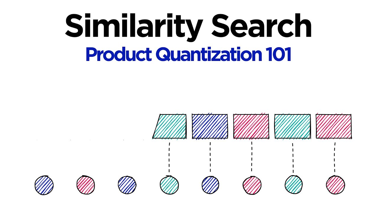
00:26:30.800 | this, and therefore improve the performance of our index. So I have one final thing to show you,

00:26:37.760 | which is how the search works in PQ. So on the right we have just a single ID vector.

00:26:47.360 | We would use our codebook, C, so that they would each go into this, like so.

00:26:59.360 | And from there we would output our quantized subvectors. So these are their reproduction

00:27:07.280 | values. Now on the left we have our query vector, and we would split that, of course,

00:27:17.600 | like we did before with our initial vectors. So we would split that, and we would get this.

00:27:28.080 | Now, what we would do is we calculate the Euclidean distance between these,

00:27:34.800 | and what we would get is we would simply add all of these up. So we'd take the product of all of

00:27:43.520 | them, hence why this is called product quantization, and the total distance would be all of those

00:27:50.800 | added together. Okay, let's say this. Now we would do that for all of our vectors. So this is a

00:28:01.680 | single, so this is like QU. That's a single quantized vector, or set of quantized subvectors.

00:28:11.120 | We need to do that for all of them. And then we just find one that produces the lowest or the

00:28:16.720 | lowest or the smallest product distance. Now, as well, it's worth noting, because we're taking

00:28:22.560 | the product, this isn't really the distance between the two vectors, between U or the

00:28:28.240 | quantized version of U and XQ, but it's almost like a proxy value for that. And then that's

00:28:38.800 | what we use to find, to identify the nearest vector. Now, I'm not going to go into the code

00:28:45.280 | behind this because it's quite long, but I am going to, I'm definitely going to record that

00:28:50.560 | and just leave it as like an extra or almost bonus video if you do want to go through that.

00:28:55.920 | But it is, it's pretty long, so I wouldn't say you necessarily need to. But in the next video,

00:29:02.240 | anyway, we're going to have a look at how we implement all this in FICE, which is obviously

00:29:07.200 | much more efficient. And it is in that video that we will also introduce the IVF and PQ

00:29:15.440 | CompSetIndex, which just allows us, if you have a look at the speed here,

00:29:19.200 | to really reduce the speed an insane amount. It's like a 90 times increase in the speed

00:29:27.760 | of our search. So it's pretty cool. But yeah, that's it for this video.

00:29:31.840 | So thank you very much for watching, and I will see you in the next one.

Product Quantization for Vector Similarity Search (+ Python)

Chapters