Stanford CS25: V1 I Transformers in Language: The development of GPT Models, GPT3

00:00:00.000 | Great. Okay, perfect. So, a sample from this model looks like this. So, they also point

00:00:11.240 | to $99.6 billion from 2004063%. It's a bunch of kind of gibberish. So, the sentence isn't

00:00:19.840 | too coherent, but at least the words do seem to be somewhat related, like they come from

00:00:24.400 | the same space. Now, jumping forward to the beginning of the deep learning boom in 2011,

00:00:31.960 | we have language modeling with neural networks now, and in particular with recurrent neural

00:00:37.040 | networks. So, we can get rid of this giant lookup table from the n-gram models, and instead

00:00:42.600 | we can have our inputs be these tokens and let this kind of recurrent cell remember some

00:00:49.240 | state and persist some state. So, if we set up a neural model like this, we get a sample

00:00:55.680 | as shown below. So, the meaning of life is the tradition of the ancient human reproduction

00:01:00.280 | is less favorable to the good boy for when to remove vigor. So, again, this doesn't really

00:01:05.780 | make any sense, but it kind of starts to have the flow of a real sentence. Yeah, so jumping

00:01:13.040 | forward even more to 2016, we have LSTM models, and of course, LSTMs are an architectural

00:01:20.520 | innovation on top of RNNs, and they have kind of better gradient flow, so they can better

00:01:26.120 | model long-term dependencies. And so, with an LSTM model, we get a sample like this with

00:01:32.740 | even more new technologies coming onto the market quickly. During the past three years,

00:01:37.320 | an increasing number of companies must tackle the ever-changing and ever-changing environmental

00:01:42.120 | challenges online. So, this sentence is starting to make a little bit of sense, though there

00:01:46.120 | are clear artifacts like the repetition of the phrase ever-changing.

00:01:50.640 | Now, starting in 2018, we have our first autoregressive transformer-based language models, which are

00:01:59.080 | even better at modeling these very long-term dependencies. And here, what I'm showing is

00:02:04.320 | an example of a completion. So, in a completion, the user supplies the prompt. In this case,

00:02:11.720 | this text swings over Kansas, and the model will continue from this prompt. So, you can

00:02:18.440 | see that this completion is coherent across multiple sentences now, though there are notable

00:02:23.840 | spelling mistakes. So, you see this like a whatever document it is, so it doesn't quite

00:02:30.520 | make sense. And now, we arrive at GPT-2, which is a 1.5-billion-parameter transformer model.

00:02:40.280 | And I copied in what I personally found was the most compelling completion from GPT-2.

00:02:45.920 | And in contrast with the last slide, what this does is it sets up a clearly fake prompt.

00:02:51.920 | So, we have something about finding unicorns and scientists in South America. And so, the

00:02:59.520 | model's probably not seen this exact prompt before and has to make up something that's

00:03:02.760 | consistent. So, the thing I find most impressive is it does so, and it's coherent across multiple

00:03:09.760 | paragraphs. It invents this fictional Dr. Perez, and it persists Perez throughout multiple

00:03:16.120 | paragraphs. And I think it's very aptly named. You have him from University of LaPaz. And

00:03:23.240 | yeah, we just have fairly coherent completions at this point. So, it's worth disclosing that

00:03:29.360 | this was the best of 10 samples. So, we still had to sample multiple times to get a sample

00:03:35.320 | like this. And finally, to end this session--

00:03:40.840 | >> Sorry, can I interrupt?

00:03:41.840 | >> Yeah, yeah, for sure.

00:03:42.840 | >> Are you talking about just examples of it failing, the worst of the 10?

00:03:45.840 | >> I can pull some up, yes. Yeah, yeah.

00:03:48.720 | >> I'm curious to know what the bad looks like.

00:03:50.320 | >> Yes, yes, yes.

00:03:51.320 | >> [inaudible]

00:03:52.320 | >> Wait, sorry, one last question. When you have these 10, you said we took the best of

00:03:58.840 | 10. That doesn't make sense.

00:03:59.840 | >> Yeah. So, this is human judged. And I'll probably expand a little bit on that for today.

00:04:04.840 | So, I want to end this kind of flyby overview with GPT-3. And since GPT-2 already produces

00:04:13.640 | such coherent text, how do you characterize GPT-3? And I would say that the best way to

00:04:19.240 | do so is that say you took the best out of five or 10 completions from GPT-2, that would

00:04:26.800 | be kind of your first completion from GPT-3. And of course, best is kind of a personal

00:04:31.960 | metric here. So, here I'm showing completion from the book Three-Body Problem. And you

00:04:41.360 | can see that the impressive things about this completion are that it really stays true to

00:04:45.760 | this style of the novel. I think the second thing that kind of impressed me was just how

00:04:52.040 | poetic like the metaphors and similes that it produces are. So, you have this stuff like

00:04:56.880 | blood was seeping through her jacket and a dark red flower was blooming on her chest.

00:05:00.720 | It's kind of like very poetic and stylistic sentences. So, it definitely understands it's

00:05:05.960 | part of a novel and it's trying to generate this kind of prose in the same style.

00:05:11.880 | So, as generated text becomes more and more coherent, I think one really...

00:05:17.120 | [inaudible]

00:05:18.120 | Yeah, yeah. So, it's 175 billion parameters versus GPT-2, which is around one billion.

00:05:26.120 | [inaudible]

00:05:27.120 | Yeah, yeah. That's a very good question. So, there's kind of... Maybe we can dive into

00:05:41.920 | it a little bit after, but there is work on kind of neural scaling laws. And so, the idea

00:05:46.000 | is like, can you predict the performance of a larger model from a series of smaller models?

00:05:50.760 | And so, I would rather characterize the increase in performance, not by kind of the small gain

00:05:54.760 | in perplexity, but like whether it lines up with the projections. And in that sense, GPT-3

00:06:00.120 | does. So, yeah, that's some intuition for... Yeah. I think personally, at OpenAI, we would

00:06:06.280 | have stopped the experiment if we did it. So, yeah.

00:06:07.280 | No, I just think it's interesting how... This is like a general thing, so we don't need

00:06:08.280 | to go into this tangent, but in machine learning, you see people pushing for like an extra,

00:06:09.280 | you know, 1% to like 0.5% accuracy, but the models are increasing in a scale that's not

00:06:22.280 | functional.

00:06:23.280 | Right, right.

00:06:24.280 | So, I wonder sometimes whether it's worth it and like where you should stop, like [inaudible

00:06:29.440 | 00:47]

00:06:30.440 | Right. Yeah. I think maybe this side we'll get to it a little bit, but there's also some

00:06:34.440 | sense in which like as you reach kind of like the entry floor of modeling, like every having

00:06:40.760 | kind of gives you like... If you think about accuracy, right, it's not on a linear scale,

00:06:46.760 | right? Like a 1% early on isn't the same as that last 1%. And so, yeah, those last bits

00:06:53.680 | really do help you squeeze a little bit out of that, you know, as accuracy, yep.

00:06:57.480 | Sorry, excuse me, but I want to ask this too.

00:07:00.480 | Oh, yes, yes. Sorry, this is accuracy. I will explain this slide. Yep. Cool. So, yep. So,

00:07:07.520 | as generated text becomes more and more realistic, I think one very natural question to ask is

00:07:12.080 | whether humans can still distinguish between real and fake text, right? And so, in here

00:07:17.040 | we have... This is, of course, like a very set up scenario. It's not... In all cases,

00:07:23.320 | the model's able to trick humans, but this is for news articles. We kind of presented

00:07:27.680 | GPT-3 generated samples against real news articles. And you can tell kind of as the

00:07:32.920 | number of parameters increases, the ability of humans to distinguish between the real

00:07:37.440 | and fake articles, that that ability goes down to near random chance. And... Oh, yes.

00:07:44.840 | How did you generate the news articles? What prompts did you use?

00:07:50.000 | I'm actually not completely sure. So, I didn't do this work particularly, but I think one

00:07:56.680 | possible approach would be to prime with a couple of news articles and then just to have

00:08:00.840 | a delimiter and just have it start generating news articles from there. Yeah. Any other

00:08:07.280 | questions? Great. So, even with all of these impressive results, I think it's worth taking

00:08:16.200 | a step back at this point and asking, "What do we really care about language modeling

00:08:20.160 | for? And what is it actually useful for?" And I think one can make the argument that

00:08:25.800 | it is actually a fairly narrow capability. Like, why would you just want some system

00:08:29.520 | that just continues text for you? And you could argue that there's more important tasks

00:08:34.320 | to solve, like summarization or translation. And I think most researchers at OpenAI would

00:08:39.400 | agree with this point of view. And in fact, GPT was not really a project that was focused

00:08:45.340 | on language modeling as an end goal, but mostly as a tool to solve a problem called unsupervised

00:08:51.480 | learning, which I'm going to go through in the next couple of slides. So, I want to do

00:08:56.240 | a history of language modeling at OpenAI and hopefully motivate why we ended up at the

00:09:01.680 | GPT series of models and kind of how we arrived there. And hopefully it'll become much more

00:09:06.920 | intuitive after this session. So, the deep learning boom started in 2012

00:09:13.440 | with AlexNet, which was a system that could take images and labels and it could classify

00:09:19.080 | images to their labels. And what we found with AlexNet was these systems were able to

00:09:24.440 | generalize surprisingly well. Like you could take data sets that weren't necessarily the

00:09:28.080 | training distribution and you still have pretty good features on. And since then, this kind

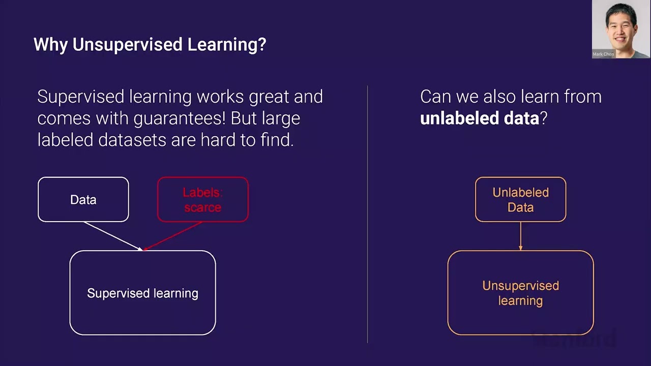
00:09:33.560 | of supervised approach has been really, really powerful, right? We've been able to train

00:09:37.720 | models in many different domains to classify very accurately. And you can even have some

00:09:43.680 | guarantees that supervised learning will work well. So, there's empirical risk minimization.

00:09:49.800 | But the problem with supervised learning is that oftentimes the labels are scarce, right?

00:09:55.000 | Especially in language tasks, there isn't really that many kind of texts paired with

00:09:58.880 | their summaries or too many pairs across languages, for instance. So, collecting a lot of data

00:10:05.880 | can be not too hard, but actually scalably labeling all of that data, it could be very

00:10:10.360 | time consuming and expensive. So, the main problem with unsupervised learning

00:10:15.120 | is can we also learn from unlabeled data? And this is a lot scarier because all of a

00:10:21.240 | sudden we're starting to optimize an objective, which isn't the one we care about downstream,

00:10:25.320 | right? So, a lot of the guarantees that we used to have, we no longer have. And we can

00:10:32.000 | only kind of hope that we learn some features that are adaptable to a wide variety of downstream

00:10:36.740 | tasks. But nevertheless, there's a reason to be very optimistic in language. And the

00:10:44.120 | reason is that there is a huge trove of unlabeled data and it's called the internet. And so,

00:10:49.280 | the real question is, can we leverage all this unlabeled data from the internet to solve

00:10:54.040 | language tasks where we don't really have that much data? And the hope is that if we

00:10:59.560 | kind of pre-train this model on the internet, you'll see all of these words used in different

00:11:03.360 | settings, kind of understand the relationships, and you'll be able to leverage this kind of

00:11:07.440 | understanding for any kind of task we do. So, now that we've established why language

00:11:14.120 | is such a good domain to try unsupervised learning in, let's talk about why use generative

00:11:19.040 | models for it and also why use autoregressive generative models. And I do want to stress

00:11:24.360 | that a lot of the guarantees you have with supervised learning are no longer there for

00:11:28.280 | unsupervised learning. So, some of these arguments will be a little bit kind of intuitive.

00:11:33.000 | And so, the first argument I want to present is this quote by Richard Feynman, which is

00:11:38.680 | pretty widespread. So, what I cannot create, I do not understand. And there's the inverse

00:11:44.080 | of this idea, which we call analysis by synthesis. And it's what I can create, I can also understand.

00:11:50.000 | And this has been studied by Josh Tenenbaum. There's definitely some kind of biological

00:11:56.840 | motivation as well for it. But the idea here is that if you're able to create a language

00:12:04.560 | model, which can generate diverse samples that are coherent, then it must also build

00:12:08.760 | up representations that can help you solve language understanding tasks. And then the

00:12:14.120 | next question is, why do we use autoregressive models? You might argue that autoregressive

00:12:19.680 | models are a kind of local objective, right? Like you're just predicting the next words.

00:12:23.960 | You could do really well with kind of some N-gram approximation, right? Why would it

00:12:29.280 | be good at solving things that allow you to summarize an entire piece of text? And so,

00:12:34.320 | an intuitive argument here could be, say that you wanted to do very well on language modeling

00:12:39.960 | for a mystery novel. And there's this grand reveal at the end, like, oh, like the culprit

00:12:45.200 | was, and then you want to predict that next token. And to do really well at that task,

00:12:50.040 | you really need to have a good understanding of what happened in the story, along with

00:12:53.440 | all the twists and turns, and maybe even some of this kind of like deductive reasoning built

00:12:57.440 | in. So the first sign of life, oh, you got a question? Oh yeah. So the first sign of

00:13:08.960 | life we had at OpenAI was in the task of predicting whether Amazon reviews were positive or negative.

00:13:14.880 | And this was work done in 2017. So instead of training a classifier in the kind of typical

00:13:20.840 | supervised way, what we did was we trained an LSTM model just to predict the next character

00:13:26.060 | in Amazon reviews. And when we trained a linear model on the features from this LSTM, what

00:13:32.120 | we found surprisingly was like one of these cells or one of these neurons was firing in

00:13:37.740 | terms of predicting sentiment. And positive activations for this neuron corresponded to

00:13:43.780 | positive reviews and negative activations to negative reviews. And this was despite

00:13:48.680 | not seeing any of the labels at training time. So you can even track kind of what this neuron

00:13:55.080 | value is across a sample. So it's a little bit hard to read, but these are reviews where

00:14:00.080 | maybe someone says, oh, I really like this film, but I didn't like this part. And you

00:14:03.240 | can kind of see the sentiment switching as you go from positive to negative. So yeah,

00:14:10.080 | just predicting the next character resulted in-- oh, yeah?

00:14:13.960 | Was there any sort of complicated architecture to encourage it?

00:14:19.360 | Oh, yeah. No, no. This was just a pure LSTM.

00:14:21.720 | Oh, yeah. So you basically looked at all the neurons and saw which ones were most--

00:14:25.000 | Yeah, in the hidden state. Yeah. So you train a linear classifier on top of that, and one

00:14:28.560 | neuron is firing with, yeah, just outsized predictive power. Yeah. Great. So next, GPT-1

00:14:36.280 | was one of the first demonstrations that this kind of approach could work broadly for text.

00:14:40.800 | So GPT-1 was trained on the internet, not on Amazon Reviews anymore, and it was fine-tuned

00:14:45.900 | on a bunch of different downstream tasks. And one thing to stress here was kind of to

00:14:51.920 | your point that the fine-tuning was very, I guess, minimally kind of-- you're not kind

00:14:58.920 | of bashing the architecture apart and kind of repurposing new modules. And it's just

00:15:04.720 | a new head that classifies for your task. And this showed that you can use this approach

00:15:11.700 | not just for semantic analysis, but also for entailment, semantic similarity, and getting

00:15:16.840 | SODAs on a lot of these benchmarks downstream. So I've already presented GPT-2 from the point

00:15:24.160 | of view of a very powerful language model. And now, I think it's worth revisiting from

00:15:28.760 | the viewpoint of unsupervised learning. So like GPT-1, GPT-2 was trained on a large chunk

00:15:34.320 | of the internet. And it's only trained to predict the next token or word from previous

00:15:39.500 | words. But the key insight of GPT-2 is that many downstream tasks can be expressed naturally

00:15:45.920 | as a language modeling task. And yeah, so GPT-2 explores how well we can perform on

00:15:51.760 | downstream tasks simply by using this method without any fine-tuning. So let me start with

00:15:56.760 | a couple of examples. So let's say you want to solve some reading comprehension benchmark.

00:16:02.280 | And this is usually set up as a prompt, which is some passage you have to read, and then

00:16:05.880 | a bunch of questions which you have to answer. So you can literally just take the entire

00:16:09.760 | prompting context. You put a question colon. You write out the question, answer colon,

00:16:15.440 | and then have the model complete from there. And this kind of gives you zero-shot reading

00:16:19.800 | comprehension. We can also use it for other tasks, like summarization. For instance, here's

00:16:26.400 | like the beginning of a CNN article about some archaeological finding. And you can just

00:16:34.160 | put TLDR after you see this passage. And the model, hopefully, if it's good enough, will

00:16:40.000 | produce good summaries. And the final example I want to show is that you can do zero-shot

00:16:47.040 | translation as well. So the way you would do this is if you wanted to convert, let's

00:16:52.480 | say, a French sentence into English, you could set up a prompt like the sentence-- insert

00:16:56.960 | the French sentence, translate it from French to English means, and then the model will

00:17:01.000 | complete. And you can sometimes do this as well.

00:17:05.240 | And one kind of critical thing to note here is that here's the chart of performance as

00:17:09.680 | you increase the number of parameters. And in all these models, they were trained on

00:17:17.000 | the same data set. So the only kind of compounding variable is scale. And you can see that as

00:17:21.120 | we scale up the models, these kind of zero-shot capabilities emerge and kind of smoothly

00:17:27.680 | get better. So the role of scale is important here. And yeah, and I think these are starting

00:17:33.640 | to approach some-- I guess they're not great benchmarks, but at least respectable benchmarks.

00:17:39.600 | Yeah, yeah, yeah, exactly. It's not going to be great in a lot of cases. And to be honest,

00:17:45.960 | the blue metric used for translation is actually often-- oh, thank you very much. It's not

00:17:52.120 | a great metric. What it does is it takes a reference solution. And basically, it does

00:17:57.920 | some kind of like n-gram comparison. So it is a big problem to have good translation

00:18:04.240 | metrics in an LP. And yeah, I think when I talk about code, I'll talk a little bit more

00:18:14.600 | about it.

00:18:15.600 | Right, so let's finally talk about how GPT-3 fits into this picture. So the primary insight

00:18:21.520 | of GPT-3 is that the training process itself can be interpreted in the context of meta-learn,

00:18:27.200 | which is kind of like learning over a distribution of tasks. And during training, what the model

00:18:32.000 | is doing is it's developing certain kind of capabilities. It's picking up some set of

00:18:38.720 | skills in terms of modeling certain passages. And during inference time, what it's doing,

00:18:45.080 | it's quickly picking up on what a task is based on what the prompt is so far, and adapting

00:18:50.960 | to that task to predict the next token.

00:18:53.360 | So you can view there's this outward loop of all the SGD steps you're doing during training,

00:18:58.760 | this inward loop of picking up on what the task is, and then modeling the next token.

00:19:04.240 | So you can imagine a lot of tasks being framed in this way. For instance, on the left, you

00:19:08.920 | can have addition. You have a lot of examples of addition in context. And hopefully, that

00:19:14.520 | would help you with a new addition problem, or you can try to unscramble a word, for instance.

00:19:20.480 | And I'll explore results on these two benchmarks in the next slides.

00:19:25.360 | So this setting we call a few-shot arithmetic. And just to explain what's going on, you're

00:19:30.600 | taking the entire context slide of your transformer, and you're putting in as many examples as

00:19:35.120 | will fit. And then finally, you put in the example that you would like to solve. So here,

00:19:42.200 | these examples could be these kind of first three addition problems, and then you have

00:19:49.240 | 31 plus 41 equals, and you ask the model to complete.

00:19:52.960 | So you notice that as the language model gets bigger, it's better able to recognize this

00:19:57.560 | task. And you can see that performance on addition, subtraction, even some kind of multiplication

00:20:03.560 | tasks increases sharply as you go towards 200 billion parameters. And there does seem

00:20:08.840 | to be some step function change right here.

00:20:12.320 | And looking at word unscrambling, this is also true. So we have parameters, again, on

00:20:19.120 | the x-axis. We have accuracy, and each of these is a different kind of unscrambled task.

00:20:23.280 | So this blue line is you do a cyclic shift of the letters, and you want it to uncycle.

00:20:28.800 | And there's a lot of other transforms you can do, like randomly inserting words, for

00:20:34.960 | instance.

00:20:35.960 | So the final point here is that this is a pretty general phenomenon. We didn't just

00:20:41.440 | test it on these two aforementioned tasks. We tried an array of, I think, 40 plus tasks.

00:20:48.620 | And here you can see how the zero shot, one shot, and few shot performance increases as

00:20:52.680 | we scale the models. So of course, they're all smoothly increasing. But one thing to

00:20:57.860 | be aware of is that the gap between zero shot and few shot is also improving as a function

00:21:02.640 | of scale.

00:21:05.600 | Awesome. So we've just seen that we can pre-train a transform-- oh, go ahead.

00:21:12.760 | Yeah.

00:21:13.760 | [INAUDIBLE]

00:21:14.760 | One is the tasks themselves that we're using. Two is the number of parameters. And then

00:21:25.360 | three, my understanding, is also the quantity of data that we've ingested.

00:21:28.060 | Yeah, yeah.

00:21:29.060 | And I was curious between those three, which ones-- you've shown a lot of-- the number

00:21:33.260 | of parameters definitely helps. I was curious, though, in terms of the degree to which also

00:21:37.900 | the training tasks and the sophistication of the tasks, as well as the quantity of data

00:21:42.200 | ingested.

00:21:43.200 | Yeah, yeah. So I guess I can dive-- maybe it's something to save for after. But yeah,

00:21:49.240 | let's dig into that after.

00:21:50.240 | [INAUDIBLE]

00:21:51.240 | Yeah.

00:21:52.240 | [INAUDIBLE]

00:21:53.240 | I guess GPT-2 and 3 aren't different. GPT-1 just has an extra classification head for

00:22:01.980 | the training tasks. Yeah. Yeah. Great, yeah. Good questions. So yeah, we've just seen that

00:22:09.220 | we can use a transformer in this pre-train and binding setup, where we have a lot of

00:22:14.780 | unlabeled data in the pre-training setting. And we have just a little bit of data in the

00:22:19.660 | binding setting.

00:22:20.660 | And we can solve a lot of language tasks in this way. And I would say this has become

00:22:25.760 | the dominant paradigm in language over the last couple of years. So there's follow-up

00:22:30.100 | objectives like BERT and T5, which have done extremely good at pushing the SOTA. But there's

00:22:35.420 | nothing really that says that these transformer models have to be applied to language. The

00:22:40.380 | transformer is a sequence model. And as such, it can just ingest any sequence of bytes and

00:22:45.620 | model them. And when you think about this, all of the data that we consume, like videos

00:22:50.180 | or audio, they're represented on our computers as sequences of bytes, right?

00:22:54.140 | And so you might think, oh, could this approach be used to just model whatever modality we

00:22:59.740 | want? And I think this kind of paradigm is very, at least interesting, when we don't

00:23:08.100 | really have good inductive biases. Like we don't [INAUDIBLE] data. But one question to

00:23:12.500 | ask is, does it even work when you do have really strong inductive biases?

00:23:16.660 | So I'm going to present some work that suggests that the answer is, yes, it still works fairly

00:23:23.280 | well in this case, in the domain of images, where convolutions are already so popular

00:23:28.660 | and proven out. And I'm going to show a second result very briefly here, which is DALI, which

00:23:34.020 | shows that it's strong enough to even ingest two different modalities and be able to jointly

00:23:39.260 | model them. So the first question is, how would you apply

00:23:44.340 | GPTU to images? And there's a few things you have to do. You have to modify this autoregressive

00:23:50.340 | next word prediction objective. So the natural analog is, you can think of images as a very

00:23:56.700 | strange language, where the words are pixels instead. And instead, you need to predict

00:24:01.860 | the next pixel at each point. And so we can just change the objective from next word prediction

00:24:06.200 | to next pixel prediction. And of course, we want this kind of large--

00:24:10.520 | [INAUDIBLE] Oh, yeah. So you just unroll it as a sequence.

00:24:17.140 | It's the same way it's stored on a computer. You just have a sequence of bytes. Yeah. Yeah,

00:24:22.300 | good question. So in the language setting, we pre-train on this large unlabeled data

00:24:27.020 | set on the internet, and we fine tune on question answering or these other benchmarks. In images,

00:24:34.420 | one good analog of this situation is you can pre-train on image net without the labels.

00:24:38.700 | You have, let's say, a low resource-- low data, sorry, setting, like CIFAR. And you

00:24:43.020 | can try to attack CIFAR classification. And of course, in both settings, you can do fine

00:24:47.700 | tuning. In GPT, you can do zero shot. And I would say the standard eval on images is

00:24:52.660 | you do linear probes. So you take features from your model. The model is frozen. You

00:24:57.340 | pass through CIFAR through the model, get some features, and you see how predictive

00:25:01.860 | these features are of the CIFAR classes. Is it kind of pixels there, which basically

00:25:08.540 | you ask a model to predict the max pixel given the-- Yeah, yeah. So pixel CNN is an instantiation

00:25:14.660 | of an autoregressive image prediction model. So what we're asking here is, can we actually

00:25:19.100 | take the same transformer architecture that we use in language, don't make any modifications

00:25:23.700 | at all, and just throw-- so there's no kind of 2D prior. So yeah, I'll call this a model

00:25:34.900 | that we train image GTC or IGPT for short. And here you can see actually what some completions

00:25:40.180 | from the model look like. So on the left column, what I'm feeding in is the pixels of the first

00:25:45.980 | half of the image. And the next four columns, what you're seeing is different model-generated

00:25:51.620 | completions. And the right column here is the original reference image. And you can

00:25:57.260 | actually see that the model is kind of doing some interesting things. If you look at the

00:26:00.740 | last two rows, it's not coming up with semantically the same completion every single time. It's

00:26:05.980 | like putting these birds in different settings, sometimes adding reflections. It's putting

00:26:10.380 | this lighthouse in grassy areas and watery areas, for instance. So if you buy into this

00:26:15.980 | philosophy of analysis by synthesis, we definitely have some hint of the synthesis part. So I

00:26:24.580 | don't have time to go through all the results with you. But I just want to say that it is

00:26:28.580 | fairly successful in this SIFAR setting where you don't have much labeled data. If you train

00:26:33.820 | a linear model on top of the features, you get better results than if you do the same

00:26:40.380 | approach with a ResNet trained on ImageNet with labels. So that's like the typical approach

00:26:44.620 | in the field. You train some ResNet on ImageNet, you get the features. Oh yeah. And if you

00:26:50.100 | compare to this approach, a generative model on ImageNet without the labels, take the features,

00:26:56.220 | it's actually better predictive of synthesis. Yeah. I'm just curious, once the architecture

00:27:01.620 | for this is the same as GPT? Oh yeah. Exactly. Yeah, yeah, yeah, yeah. It's the GPT architecture.

00:27:09.500 | So you can modify GPT to have 2D bias. You can do 2D position embeddings. Well, we don't

00:27:14.580 | do that. We just want to see, can you use the same exact approach? So early use of the

00:27:20.180 | data is just sequential. Yeah. But also there's metadata showing about how that sequential

00:27:23.980 | should be reconstructed. Like what's the weight, for example. Oh, can you explain? So the data

00:27:32.340 | on this stored, but when you want to transform that sequence into an image, you have metadata

00:27:38.180 | that will say something like, just like in NumPy arrays, it'll say, here's the strike.

00:27:41.780 | So here's how to rearrange it. I see. What I'm curious to notice is GPT, before it's

00:27:47.280 | given an image, at least given this metadata. I see, I see. Okay. Yeah, that's an extremely

00:27:52.020 | good question. I don't know how this problem is solved. Yeah, yeah, yeah. In this case,

00:27:57.840 | all the images have the same shape. Oh, okay, okay. Yeah, but we don't tell it the concept

00:28:05.020 | of row within the model. Yeah, but all images are the same shape. Yeah, so it needs to learn

00:28:09.460 | it from the data, but yeah, the data looks the same. Got it. Yeah. It'll be interesting

00:28:13.100 | if it's variable image shapes, then it's going to be interesting to do it. Yeah, yeah. Cool.

00:28:21.660 | Are there a lot more pixels than there are token sizes in the context there? Yeah, so

00:28:26.740 | this is a pretty low resolution images. Yeah, so we can actually, the models we're comparing

00:28:33.380 | against are trained on kind of high resolution images. So I think that makes it even more

00:28:37.140 | impressive. But yeah, we're just training at 32 by 32 resolution. Yeah. Cool. So if

00:28:44.580 | we fine tune these models for CIFAR classification, we can get 99% accuracy, which matches G-pipe.

00:28:50.980 | And this is G-pipe, for instance, is a system which is pre-trained on ImageNet with labels

00:28:55.860 | and then also fine tuned with labels. So yeah, it just kind of shows you like even this approach,

00:29:01.620 | which doesn't really know about convolutions can do well. I think you're going to hear

00:29:05.260 | more about that next week with Lucas' talk. Cool. So by now, it shouldn't be surprising

00:29:12.860 | at all that you can model a lot of different modalities with transformers. So in DALI,

00:29:17.940 | we just asked, what about throwing two different modalities at the model and seeing if it can

00:29:23.180 | learn kind of how to condition on text to produce an image. And for instance, one thing

00:29:29.380 | you might want it to do is like you provide one of these text captions and you want it

00:29:33.340 | to generate some image like the one below. And the easy way to do this is just train

00:29:37.740 | a transformer on the concatenation of a caption and an image. And of course, in a lot of these

00:29:43.460 | situations, the idea is very simple, but the implementation and execution is where the

00:29:48.540 | difficulty is. And I'm not going to talk too much about that. I think the focus today is

00:29:52.340 | on language, but you can refer to the paper for a lot of those details.

00:29:56.140 | Oh, yeah. So you have a max caption length and you just kind of cut it off at that length

00:30:08.620 | and you can pad up to that. Right. So you can see that it can generate fairly good samples.

00:30:16.900 | So if you want like a storefront with the word "OpenAI" on it, it's not perfect, but

00:30:21.540 | it's understood at least it's kind of like reverse OCR problem where you take some text

00:30:26.300 | and render it. And it's kind of typically rendering it in like office looking places.

00:30:31.140 | So that's one encouraging sign. But I do think my favorite results here are zero-shot image

00:30:38.380 | transformation. So what's going on here is, for instance, if your prompt is the exact

00:30:42.940 | same cat on the top as a sketch on the bottom and you feed in the top half of it, this image,

00:30:48.820 | which is a cat, and you ask it to complete the rest of the image, then it'll render the

00:30:53.780 | top cat actually as like a sketch. And you can do the same thing with like flipping over

00:30:59.580 | photos, for instance. You can zoom in to a photo. Of course, they're not perfect, but

00:31:05.260 | it has some understanding of what the text is trying to do.

00:31:08.500 | In the captions originally, like the training, in the training set, do they have like wording

00:31:14.740 | such as extreme close up view? I think that is the, it probably are some

00:31:20.820 | examples like that. And that's probably where it's picking up some of this knowledge from.

00:31:23.940 | Though we don't seek out these examples. It's just, yeah, yeah, exactly.

00:31:28.860 | Okay. Perfect. Yeah. So this is just how we just go and do a massive web script. There's

00:31:36.620 | no kind of, we're not trying to find examples like this. Right. And so you can also do things

00:31:41.940 | like colorization, right? You can take the cat color red, and this has to kind of recognize

00:31:46.560 | that what the object is in the figure. And yeah, and here you can do stuff like semantic

00:31:53.620 | transformations, like adding sunglasses into the cat, and you can put it on postage, for

00:31:58.980 | instance. Yeah. So it's remarkable that you can do a lot of these, like transform zero

00:32:03.420 | shot. It wasn't trained to do these things specifically. Cool. So moving on, the last

00:32:13.060 | section of my talk today is on codex, which is our most recently released code writing

00:32:17.380 | models. And the first question you should rightly

00:32:21.420 | ask here is why, why train them all on code anyway? Isn't at this point, isn't it just

00:32:27.340 | another modality and what is the novelty that there is at this point? Right. So let me give

00:32:33.820 | you a couple of reasons. So the first is that GPT-3, it had a rudimentary ability to write

00:32:39.820 | Python code already from a doc string or descriptive method name. And we actually didn't train

00:32:45.420 | it on much code data. Actually, I think there might've been active filtering to get rid

00:32:49.540 | of code data. And so we were surprised that there was this capability anyway. So that,

00:32:53.820 | you know, like if we actually purpose the model and trained it on the large amount of

00:32:57.620 | code that we can find, maybe something interesting will happen there. Next, what sets apart code

00:33:03.740 | from other modalities is that there is a kind of ground truth correctness of a sample and

00:33:09.660 | functions can be tested with unit tests and an interpreter. So this is very different

00:33:14.140 | from language, whereas to get a ground truth, you might need a human to come in. And even

00:33:18.500 | then sometimes humans won't agree like this, this is the better sample or this isn't the

00:33:22.940 | better sample. And the last thing is I used to dabble in competitive programming myself

00:33:27.380 | and yeah, I really wanted to create a model that could solve problems that I could. So

00:33:34.660 | yeah, we wrote a paper on it too. So yeah. I think it's kind of a high-level programming

00:33:50.020 | language which is similar to our human language. Have you guys ever tried to predict some even

00:33:57.860 | lower level languages like CPP? Yeah. I think there's, yeah, there's follow-up work where

00:34:06.100 | we just train on a bunch of different languages and I don't know the metrics off the top of

00:34:10.700 | my head, but I have seen some assembly writing models. Yeah. Cool. So I guess, yeah, continue

00:34:20.740 | on the third from before. So we have this setting where we have unit tests and interpreter.

00:34:25.860 | So how do we actually evaluate these models in a way that's kind of aware of these two

00:34:30.660 | concepts? So the first thing we did was we have a data set, a new data set, which is

00:34:34.900 | 164 handwritten programming problems. And these kind of have the format shown here.

00:34:41.140 | Like there's a function name, a doc string, there's a solution and there's an average

00:34:45.980 | of around eight units per problem. And why is it important that we hand wrote these?

00:34:50.220 | Well, the thing is we're training on such a large part of GitHub. Like if you said,

00:34:54.780 | okay, I'm going to take like some B code problems and I'm going to turn them into an evaluation,

00:34:59.260 | that's not going to work because there's just so many GitHub repos that are like, oh, here's

00:35:02.700 | the solution to this B code problem. So while this doesn't kind of guarantee that this problem

00:35:07.340 | isn't duplicated, at least someone wrote it without trying to copy it from another source.

00:35:14.780 | So here's some kind of examples of a unit test that you would evaluate the previous

00:35:20.060 | function on. I think it should be fairly clear that we should be using this metric. This

00:35:26.060 | is the correct kind of ground truth metric to use. I mean, humans do use unit tests to

00:35:30.260 | evaluate code. And I would say if you're familiar with competitive programming, you can't manually

00:35:35.420 | judge all like tens of thousands of submissions that are coming in. You need the unit tests

00:35:39.860 | and that is a fairly good filter. So one interesting point here was we had to

00:35:44.980 | create a sandbox environment to run these kind of generated solutions in. Because when

00:35:50.180 | you train on GitHub, there's a bunch of malicious code. There's a bunch of kind of insecure

00:35:53.900 | code. You know, all your models should be sampling that and kind of running that on

00:35:57.060 | your environment. Cool. So now that we have an evaluation data

00:36:02.620 | set, let's define a metric. And so the metric we're going to use is called pass at K. And

00:36:08.540 | the definition is the average probability over all the problems that at least one out

00:36:12.980 | of two samples passes the unit test. So if we evaluate this metric by just taking every

00:36:20.500 | problem and exactly generating K samples, it's actually not, there's high variance just

00:36:26.980 | kind of sampling in that way. But you imagine the pass rate of a particular sample is around

00:36:30.780 | one over K. This is kind of like an all or nothing metric. So what we do instead is we

00:36:36.940 | generate a much larger set of samples and greater than K. Most of the times it's like

00:36:41.580 | greater than 5K. And we count the number that are correct and we compute this unbiased estimator.

00:36:48.100 | And it looks more complicated than it actually is. It's just complimentary counting. You

00:36:52.620 | take kind of the number of combos where all of them fail. Cool. So then we train our model.

00:37:02.580 | And like I alluded to earlier, there's 160, about 160 gigabytes of code, which is collected

00:37:09.900 | from 54 million repositories. For efficient training, what we did was we fine tuned from

00:37:15.260 | GPT-3 models of various sizes. And this isn't actually strictly necessary. We find that

00:37:20.620 | we can get to roughly the same final loss and performance without this, but it is slower

00:37:26.020 | to do it without the super training stuff. And so we already have these models, why not

00:37:30.900 | just fine tune them? And one extra trick to make training much faster here is in code,

00:37:36.660 | there's a lot of runs of spaces, right? And those don't get compressed efficiently in

00:37:40.940 | language because you just don't see them very often. So they typically get broken up into

00:37:46.140 | like many separate tokens. So we introduce additionally some tokens that compress runs

00:37:52.220 | of that space. And that makes training maybe like 30 or 40% more efficient.

00:37:57.340 | Yeah, exactly. Yeah. Great. So once we have these models, we can go and revisit the human

00:38:07.620 | eval data set. And I can share a couple of problems to give you a sense of where the

00:38:12.140 | models are at and also what kind of difficulty level the problems in the data set are at.

00:38:18.440 | So this is a 12 billion parameter model that passed out 90%, which means that 90% of the

00:38:23.700 | samples will pass the unit test. And this is something like anyone doing a first day

00:38:29.620 | of Python would be able to do. So you increment all the elements of a list by one. Here's

00:38:36.780 | a problem where the pass rate is 17%. So this is the problem I gave earlier. So you are

00:38:42.820 | given a non-empty list of integers. You want to return the sum of all odd elements that

00:38:46.820 | are in even positions. And this might not sound that much harder to you, but models

00:38:49.820 | can often get confused about like, "Oh, is odd referring to positions or elements?" And

00:38:55.300 | so here you can actually see that it's doing the right thing.

00:39:00.980 | And finally, this is an example of one of the harder problems in the data set. So the

00:39:05.460 | pass rate is under 1% here. And so what's going on here is actually there's an encode

00:39:09.500 | function which takes a string. It chunks it up into groups of three characters and it

00:39:14.460 | does a cyclic shift on each character. And you have to write a decoder, something that

00:39:18.500 | reverses this operation. So you can see that the model, this is a real model solution.

00:39:24.940 | So it chunks up the characters in the same way. You can see that the cyclic shift is

00:39:29.340 | the opposite way. So up there, it takes the first element of each group, moves it to the

00:39:34.540 | end, and now it takes the last element of each group, moves it to the end.

00:39:39.540 | Okay. So I'm wondering what's the effect of... So you had a couple of examples in the previous

00:39:45.340 | slide, but you didn't give us in the comments. So I'm wondering if the model will be able

00:39:49.540 | to extrapolate what it's doing by the examples on its own and not relying on the distribution.

00:39:55.100 | Right. Yeah. So some of our tasks, there are some examples in the doc string, and some

00:39:59.860 | of them don't. I think it's just to kind of match the distribution of real kind of tasks

00:40:04.820 | we find in the real world. Like in this case, it doesn't have it, but definitely for the

00:40:09.340 | unit tests, none of those appear within...

00:40:11.780 | I'm just curious if you just give it the examples and not be able to distribute all the tasks.

00:40:17.860 | Oh, I see. I see. So can it do like pure induction where you don't tell the task at all? Yeah.

00:40:23.980 | I haven't tried it, to be honest. I think it's worth a shot. Yeah. Thanks.

00:40:30.460 | Yep. So yeah, at this point, we've trained codex models, we've evaluated on this metric,

00:40:37.020 | but the thing is, was it worth all this trouble? You already have these metrics like blue that

00:40:42.460 | are match-based in language. Couldn't we have just used this to approximate it? We don't

00:40:47.420 | need an interpreter, we don't need to generate so many samples. And it would be great if

00:40:52.140 | it kind of separated out like this. But what we find is that this is, if you take four

00:40:59.260 | random problems from human data, and you plot the distribution of blue scores for correct

00:41:04.460 | and wrong solutions, you actually find a lot of distributional overlap, right? It's hard

00:41:09.500 | to distinguish the green from the blue distribution. And so this suggests that blue actually isn't

00:41:16.340 | a very good metric for gauging functional correctness, and that we actually do need

00:41:20.060 | this new kind of metric and this new data set.

00:41:27.140 | So now let's explore the setting where in PASAC-K, K is greater than one. And so the

00:41:33.620 | first observation we have here is that the temperature that you sample at, it affects

00:41:39.260 | your PASAC-K. And just for some intuition, if you do temperature zero sampling, you're

00:41:44.500 | going to get the same sample every single time you're doing hard fact sampling. So it

00:41:48.220 | doesn't matter how many samples you generate, you're just going to get the same PASAC-K.

00:41:53.460 | But if you want to generate a hundred samples, you can afford to make some mistakes. You

00:41:58.420 | just want a very diverse set of samples. So you can up the temperature. You can see kind

00:42:02.820 | of as you up the temperature, the slope of the kind of number of samples against pass

00:42:07.260 | rate, it becomes steeper. And so you can kind of take the upper hull of this and you can

00:42:12.300 | find the optimal temperature for each number of samples.

00:42:19.180 | And so this brings me to personally my favorite result of the paper, which I call the unreasonable

00:42:23.940 | effectiveness of sampling. And so let me explain what's going on here. So this is the number

00:42:28.720 | of parameters in the model, and here you have pass rate at one and a pass rate at a hundred.

00:42:34.100 | And the reason I use this term unreasonable effectiveness is that I think there's a world

00:42:38.700 | where if the orange line and the blue line weren't that far apart, I might not be that

00:42:44.260 | surprised. At these scales, the model, it rarely makes kind of syntactical errors anymore.

00:42:49.020 | Like if you run it, it'll run and produce some kind of output. So you could imagine

00:42:53.260 | a world where basically what you're doing, the model has some approach in mind. It's

00:42:57.340 | just repeatedly sampling that approach and it's just either right or wrong. But instead,

00:43:01.580 | what we find is that the model is actually composing different parts and producing functionally

00:43:06.580 | different things. And you get this huge boost from under 30% to over 70% just by sampling

00:43:13.460 | a lot of samples from the model.

00:43:18.740 | So unfortunately, knowing that one of your samples is correct, it isn't that useful if

00:43:23.940 | you don't have access to the unit tests. And one setting where, practical setting where

00:43:30.100 | you would care about this is say you're creating an autocomplete tool, right? And you generate

00:43:34.460 | a hundred samples, but you don't want to show your user a hundred samples and have them

00:43:38.300 | pick one, right? You want to kind of try to pre-filter, but you don't have unit tests.

00:43:43.940 | So can we kind of approximate this Oracle sampling with some other ranking heuristic?

00:43:50.500 | So here I'm showing a couple of different heuristics. You can randomly pick one, but

00:43:55.780 | the one that seems most promising is to rank by mean probability. And I know it's kind

00:44:03.460 | of maybe not theoretically well grounded, but in language, this kind of heuristic is

00:44:08.500 | fairly strong as well.

00:44:13.540 | So recall that what we're doing is we have this evaluation set where we have kind of

00:44:18.260 | standalone functions. We want to produce solutions to that. But when we're doing training, there's

00:44:24.260 | a lot of code that isn't relevant for this task. For instance, there's a lot of classes

00:44:28.600 | that we're seeing. There's actually data classes too, which aren't relevant at all. And actually

00:44:32.820 | there's a lot of incorrect code on GitHub too. So we might be modeling incorrect solutions

00:44:37.780 | as well as correct ones. So one thing we thought was let's fine tune codecs on further on a

00:44:44.780 | couple of data sets where they are standalone functions and you have kind of more guaranteed

00:44:50.780 | correct solutions to that.

00:44:52.740 | So what we did was we found these problems from a couple of sources. So one is competitive

00:44:57.820 | programming problems. You can kind of go on these sites. Oftentimes they'll just give

00:45:01.780 | you the unit test. Sometimes when they don't give you the unit test, you can submit incorrect

00:45:05.500 | solutions and they'll tell you the first one you failed on and then you can kind of keep

00:45:08.580 | inserting that in. So you can get a lot of competitive programming problems. And another

00:45:14.740 | source is projects where continuous integration is enabled. So why are these useful? Because

00:45:21.620 | you can actually kind of do an execution tracing. So when you run the integration tests, you

00:45:27.220 | can get all the inputs to functions that are called and their outputs as well. And so you

00:45:31.540 | actually have the true function body. You know what the test output is supposed to be.

00:45:35.140 | You know, kind of the ground truth inputs and outputs. And these are kind of like two

00:45:39.540 | orthogonal data sets. One kind of helps you with like algorithmic kind of tasks. And one

00:45:44.420 | is more kind of like, can I manipulate command line utilities and tasks like that.

00:45:52.260 | So this brings us to the main figure of the codecs paper. So really what we're seeing

00:45:57.020 | is a progression of capability. So with GPT-3 on this human eval data set, the pass rate

00:46:02.380 | at one is zero. Basically you can generate like one or two lines coherently, never really

00:46:07.940 | a whole program coherently. Now when you fine tune on code, which is codex, this orange

00:46:14.340 | line, you start to see some kind of non-noticeable performance on this data set. When you do

00:46:19.260 | this additional supervised fine tuning, that's this green line, you get even better pass

00:46:24.500 | rates. And then if you kind of generate a hundred samples from this model, re-rank with

00:46:30.380 | mean log P, even better pass rates. And finally, of course, if you have access to an Oracle,

00:46:35.180 | it gives you the best pass rates.

00:46:36.740 | So I have one question here. So can you actually use a re-ranking to like, like for the, to

00:46:41.020 | the model? Can you use it for like as a backdrop signal?

00:46:43.900 | Yeah, yeah. So we've explored that. I don't know if I can say too much about these results.

00:46:53.420 | And finally, I don't want to suggest that these, these models are perfect. They have

00:46:56.780 | a lot of limitations that human programmers don't run into. So one is like, actually all

00:47:02.420 | generative models are autoregressive generative models, kind of, we have some problems with

00:47:06.780 | binding. So when there's like a lot of variables going on, like a lot of operations going on,

00:47:10.860 | sometimes it's like hard to figure out which operation is binding to which variable. So

00:47:14.620 | you can kind of see some examples of that on the left. And one other kind of counterintuitive

00:47:19.300 | behavior is composition. So we can take a bunch of very simple building blocks, like

00:47:23.740 | take a string and reverse it, or, or like delete every third character or something.

00:47:28.220 | And assuming like, if you can chain two of these operations, you could probably chain

00:47:31.220 | 10 of them, but our models aren't able to do that yet.

00:47:37.540 | Cool. So moving on to the conclusion, we have four main points in today's talk. So first

00:47:45.180 | progress in neural language modeling has been fairly rapid. And at GPT, it wasn't the result

00:47:50.140 | of a push on language modeling and more of a result of work on pushing unsupervised learning

00:47:55.460 | in language. The third point is that autoregressive modeling is universal and it can yield strong

00:48:01.660 | results even when there are strong adaptive biases, like in images or in text. And finally,

00:48:08.180 | we can produce strong co-generating models by fine tuning GPT3 on code. And sampling

00:48:13.620 | is an unreasonably effective way to improve model performance. Cool. And to end with some

00:48:19.700 | acknowledgments, I want to thank my CodeX primary co-authors, some mentors at OpenAI

00:48:25.700 | and the algorithms team, which I have worked very closely with. Great. Thank you guys for

00:48:30.580 | your attention.

00:48:32.460 | Thanks.

00:48:33.460 | Bye.

00:48:33.460 | [BLANK_AUDIO]

Stanford CS25: V1 I Transformers in Language: The development of GPT Models, GPT3

Chapters