Machine Learning 1: Lesson 11

00:00:00.000 | So let's just yeah, let's start by reviewing

00:00:03.080 | Kind of what we've learned about

00:00:06.160 | optimizing

00:00:08.840 | Multi-layer functions with SGD and so the idea is that we've got some data and

00:00:14.740 | Then we do something to that data. For example, we multiply it by a weight matrix

00:00:21.820 | And then we do something to that

00:00:26.280 | for example, we put it through a softmax or a sigmoid and

00:00:30.200 | Then we do something to that such as do a cross entropy loss or a root mean squared error loss

00:00:39.200 | Okay, and that's going to like give us some scalar

00:00:46.660 | So this is going to have no hidden layers this has got a linear layer

00:00:56.440 | A nonlinear activation being a softmax and a loss function being a root mean squared error or a cross entropy

00:01:03.420 | All right, and then we've got our input data

00:01:06.920 | Put linear nonlinear

00:01:13.300 | loss

00:01:16.280 | so for example if this was

00:01:19.440 | sigmoid or

00:01:25.320 | Or softmax and this was cross entropy then that would be logistic regression

00:01:31.420 | So it's still yeah

00:01:36.640 | Cross entropy. Yeah, let's do that next sure

00:01:42.840 | For now think of it like think of root means great error same thing some loss function. Okay now

00:01:49.880 | We'll look at cross entropy again in a moment

00:01:52.880 | So

00:01:54.880 | How do we calculate the derivative of that with with respect to our weights, right?

00:02:05.120 | So really it would probably be better if we said

00:02:07.840 | X comma W here because it's really a function of the weights as well. And so we want the derivative of this

00:02:17.440 | With respect to our weights

00:02:22.380 | Sorry, I put it in the wrong spot

00:02:27.380 | G f of X comma W

00:02:32.700 | I just screwed up. That's all that's why that didn't make sense. All right

00:02:38.480 | So to do that we just basically we do the chain rule so we just say that this is equal to H of

00:02:48.740 | you and

00:02:52.340 | you

00:02:54.340 | Equals

00:02:56.540 | G F of G U equals

00:03:00.480 | G of V and

00:03:04.180 | V equals F of

00:03:06.740 | X

00:03:08.660 | So we can just rewrite it like that

00:03:10.460 | Right and then we can do the chain rule so we can say that's equal to H - the derivative is H - you by

00:03:18.260 | G - V by

00:03:21.660 | F - X

00:03:23.660 | Happy with all that so far. Okay, so

00:03:27.900 | In order to take the derivative with respect to the weights therefore

00:03:33.940 | We just have to calculate that derivative with respect to W using that exact formula

00:03:41.380 | So if we had in there

00:03:44.260 | Yeah

00:03:47.780 | so

00:03:49.780 | Yeah, so so D of all that dW would be that yeah

00:03:58.280 | So then if if we you know went further here and

00:04:05.440 | Had like

00:04:09.780 | Another linear layer, right? Let's give us a bit more room

00:04:17.740 | now the linear layer I

00:04:19.740 | Cover

00:04:24.100 | W2

00:04:27.540 | Right, so we have another linear layer

00:04:30.380 | There's no difference to now calculate the derivative with respect to all of the parameters. We can still use the exact same

00:04:39.740 | chain rule, right

00:04:42.700 | So so don't think of the multi-layer network has been like things that occur at different times

00:04:49.140 | it's just a composition of functions and

00:04:51.500 | So we just use the chain rule to calculate all the derivatives at once, you know

00:04:58.080 | There's a they're just a set of parameters that happen to appear in different parts of the function

00:05:02.540 | but the calculus is no

00:05:04.540 | No different so to calculate this with respect to

00:05:09.660 | W1 and W2, you know, it's it's just you just increase

00:05:14.500 | You know W you can just now just call it W and say W1 is all of those weights

00:05:20.020 | So the result that's a great question so what you're going to have then

00:05:28.220 | is

00:05:31.780 | A list of parameters, right? So

00:05:38.460 | Here's W1 and like it's it's it's probably some kind of higher rank tensor, you know, like if it's a

00:05:47.500 | convolutional layer

00:05:49.740 | It'll you know be like a rec 3 tensor or whatever, but we can flatten it out that we just make it a list of parameters

00:05:57.340 | There's W1. Here's W2

00:05:59.940 | Right. It's just another

00:06:02.100 | list of parameters, right

00:06:04.100 | And here's our loss

00:06:06.580 | Which is a single, you know a single number

00:06:09.020 | so therefore

00:06:11.620 | our derivative

00:06:13.820 | Is just a vector of that same length, right?

00:06:17.940 | It's how much does changing that value of W affect the loss how much does changing that value of W affect the loss?

00:06:24.740 | Right, so you can basically think of it as a function like, you know y equals

00:06:31.260 | ax 1 plus BX 2

00:06:36.100 | Plus C right and say like oh, what's the derivative of that with respect to A B and C?

00:06:42.300 | And you would have three numbers the derivative with respect to A and B and C and that's all this is right

00:06:49.080 | It's a derivative with respect to that weight that weight and that weight and that weight and that weight that way

00:06:52.860 | To get there inside the chain rule

00:07:00.700 | We had to calculate and I'm not going to go into detail here, but we had to calculate like

00:07:05.780 | Jacobians so like the derivative

00:07:08.780 | when you take a matrix product is

00:07:11.940 | you've now got something where you've got like a

00:07:14.980 | weight matrix and

00:07:18.060 | You've got an input vector. These are the activations from the previous layer, right and you've got

00:07:29.220 | some new

00:07:31.100 | output activations, right and so now you've got to say like okay for this particular sorry for this particular

00:07:37.920 | weight

00:07:41.220 | How does changing this particular weight change?

00:07:46.860 | This particular output and how does changing this particular weight change this particular output and so forth so you kind of end up with these

00:07:56.740 | Higher dimensional tensors showing like for every weight. How does it affect?

00:08:01.620 | Every output, right?

00:08:04.340 | But then by the time you get to the loss function the loss function is going to have like a mean or a sum or something

00:08:10.180 | so they're all going to get added up in the end, you know, and so this kind of thing like I

00:08:16.540 | don't know it drives me a bit crazy to try and

00:08:19.660 | Calculate it out by hand or even think of it step by step because you tend to have like

00:08:26.660 | You just have to remember for every input in a layer for every output in the next layer

00:08:31.020 | You know, you're going to have to take out for every weight for every output. You're going to have to have a separate

00:08:37.460 | gradient

00:08:40.300 | One good way to look at this is to learn to use pytorches like dot grab

00:08:47.620 | Attribute and dot backward method manually and like look up the tutorial the pytorch tutorials

00:08:53.460 | and so you can actually start setting up some calculations with a vector input and the vector output and then type dot backward and

00:09:00.120 | Then say type dot grad and like look at it

00:09:03.900 | Right and then do some really small ones with just two or three

00:09:06.540 | items in the input and output vectors and like make the make the operation like plus two or something and like

00:09:13.140 | See what the shapes are make sure it makes sense

00:09:16.700 | Yeah, because it's kind of like

00:09:19.540 | this

00:09:22.660 | Vector matrix calculus is not like introduces zero new concepts to anything you learned in high school

00:09:29.620 | Like strictly speaking but getting a feel for how these shapes

00:09:34.580 | Move around I find talk a lot of practice, you know, the good news is you almost never have to worry about it

00:09:42.900 | Okay, so

00:09:49.660 | We

00:09:51.660 | Were

00:09:55.260 | Talking about then using this kind of logistic regression

00:10:00.580 | For NLP and before we got to that point we were talking about using naive base for NLP

00:10:10.460 | And the basic idea was that we could take a

00:10:15.060 | document

00:10:17.020 | Right a review like this movie is good and turn it into a bag of words

00:10:22.380 | Representation consisting of the number of times each word appears

00:10:26.380 | All right, and we call this the vocabulary. This is the unique list of words. Okay, and we used the

00:10:33.860 | SK learn count vectorizer to automatically generate both the vocabulary which in SK learn they call they call the features

00:10:43.300 | And to call create the bag of words representations and the whole group of them then is called a term document

00:10:49.940 | matrix, okay

00:10:52.700 | And we kind of realized that we could calculate

00:10:55.860 | the probability that

00:10:58.780 | a

00:11:01.860 | positive review contains the word this by just

00:11:05.260 | averaging the number of times this appears in the positive reviews and we could do the same for the

00:11:13.260 | Negatives right and then we could take the ratio of them to get something which if it's greater than one

00:11:19.900 | was a

00:11:21.940 | Word that appeared more often in the positive reviews or less than one was a word that appeared more often in the negative reviews

00:11:28.700 | okay, and

00:11:31.420 | Then we realized you know using using Bayes rule that and taking the logs

00:11:37.920 | That we could basically end up with something where we could add up the logs of these

00:11:43.820 | Plus the log of the ratio of the probabilities that things are in class 1 versus class 0

00:11:49.680 | And end up with something we can compare to 0

00:11:53.580 | It's a bit greater than 0 then we can predict a document is

00:11:58.020 | Positive or if it's less than 0 we can predict the document is negative and that was our Bayes rule, right?

00:12:04.140 | So we kind of did that from math first principles

00:12:09.020 | And I think we agreed that the the naive in naive Bayes was a good description

00:12:14.260 | Because it assumes independence when it's definitely not true

00:12:17.980 | but it's an interesting starting point and I think it was interesting to observe when we actually got to the point where like

00:12:24.780 | Okay, now we've you know calculated

00:12:27.040 | the the ratio of the probabilities and

00:12:31.420 | Took the log and now rather than multiply them together of course we have to add them up and

00:12:37.580 | When when we actually wrote that down we realized like oh that is

00:12:42.580 | You know just a standard

00:12:46.260 | Weight matrix

00:12:50.660 | product plus a bias

00:12:52.780 | Right and so then we kind of realized like oh, okay, so like if this is not very good

00:12:58.860 | accuracy 80% accuracy

00:13:04.380 | Why not improve it by saying hey, we know other ways to calculate a

00:13:09.180 | You know a bunch of coefficients and a bunch of biases, which is to

00:13:14.400 | Learn them in a logistic regression right so in other words this this is the formula we use for a logistic regression

00:13:22.520 | And so why don't we just create a logistic regression and fit it

00:13:28.520 | Okay, and it's going to be

00:13:32.060 | Give us the same thing, but rather than

00:13:34.240 | Coefficients and biases which are theoretically correct based on you know this assumption of independence and based on Bayes rule

00:13:42.620 | There'll be the coefficients and biases that are actually the best in this data

00:13:48.100 | All right, so that was kind of where we got to and so

00:13:52.740 | The kind of key insight here is

00:13:57.340 | like

00:14:00.740 | Just about everything I find a machine learning ends up being either like a tree or

00:14:07.260 | You know a bunch of matrix products and monomerities

00:14:11.380 | Right like it's everything seems to end up kind of coming down to the same thing

00:14:16.540 | Including as it turns out Bayes rule, right?

00:14:20.620 | And then it turns out that nearly all of the time then whatever the parameters are in that function

00:14:28.820 | Nearly all the time it turns out that they're better

00:14:30.820 | learned than

00:14:33.460 | Calculated based on theory right and indeed that's what happened when we actually tried learning those coefficients

00:14:39.780 | We got you know 85 percent

00:14:42.300 | So then

00:14:46.300 | We noticed that we could also rather than take the whole term document matrix

00:14:51.180 | We could instead just take them the you know ones and zeros for presence or absence of a word

00:14:57.420 | And you know sometimes it was you know, this equally is good

00:15:01.460 | But then we actually tried something else which is we tried adding regularization

00:15:06.260 | And with regularization the binarized approach turned out to be a little better. All right, so then

00:15:12.540 | regularization

00:15:15.220 | Was where we took the loss function?

00:15:17.220 | And again, let's start with RMSE and then we'll talk about cross entropy loss function was

00:15:24.960 | Our predictions minus our actuals sum that up take the average

00:15:34.520 | Plus a

00:15:38.600 | Penalty

00:15:41.680 | Okay, and so this specifically is the L2 penalty

00:15:45.300 | If this instead was the absolute value of W

00:15:50.280 | Then that would be the L1 penalty. Okay?

00:15:54.400 | um

00:15:56.400 | We also noted that we don't really care about the loss function per se we only care about its derivatives

00:16:05.400 | That's actually the thing that updates the weights

00:16:07.400 | so we can because this is a sum we can take the derivative of each part separately and so the derivative of this part was just

00:16:15.760 | that

00:16:18.320 | Right, and so we kind of learned that even though these are mathematically equivalent

00:16:22.920 | They have different names

00:16:24.560 | This version is called weight decay and it's kind of what's used that term is used in the neural net picture

00:16:31.100 | Okay

00:16:33.600 | So cross entropy on the other hand, you know, it's just another loss function like root mean squared error

00:16:40.960 | But it's specifically designed for

00:16:52.280 | classification

00:16:54.200 | And so here's an example of

00:16:56.200 | Binary cross entropy. So let's say this is our you know, is it a cat or a dog? So let's just say is cat

00:17:02.400 | one or a zero so cat cat dog dog cat and these are our

00:17:07.960 | Predictions this is the output of our final layer of our neural net or a logistic regression or whatever

00:17:15.000 | all right, then

00:17:18.320 | All we do is we say okay. Let's take

00:17:21.840 | the

00:17:23.840 | the actual

00:17:25.640 | times the log of the prediction and

00:17:27.640 | Then we add to that 1 minus actual times the log of 1 minus the prediction and then take the negative of that whole thing

00:17:35.680 | All right

00:17:39.200 | So I suggested to you all that you tried to kind of write the if statement version of this

00:17:45.800 | So hopefully you've done that by now. Otherwise, I'm about to spoil it for you. So this was

00:17:51.320 | y

00:17:52.640 | times log

00:17:54.640 | y

00:17:56.480 | plus

00:17:58.000 | 1 minus y times log

00:18:01.320 | 1 minus y

00:18:04.520 | Right and negative of that. Okay, so who wants to tell me how to write this is an if statement

00:18:16.560 | She hit me. I'll give a try. So if y equal to

00:18:21.480 | Sorry, if y equal to 1

00:18:24.280 | Then return log y. Mm-hmm

00:18:27.640 | otherwise

00:18:29.680 | Well else return log 1 minus 1. Good. Oh, that's the thing in the brackets and you take C minus

00:18:37.280 | Good. So the key insight she's using is that y has two possibilities 1 or 0

00:18:42.640 | Okay, and so very often the math

00:18:46.080 | Can hide?

00:18:47.760 | The key insight which I think happens here until you actually think about what the values it can take

00:18:53.000 | right, so

00:18:55.720 | That's that's all it's doing it's saying either give me that or give me that

00:19:01.520 | Right. Could you pass that to the back place tension?

00:19:05.360 | If I'm missing something, but do you know the two variables in that statement because you got why?

00:19:13.400 | Shouldn't be like white hot in the way. Oh, yeah. Thank you

00:19:17.020 | As usual, it's me missing something

00:19:22.120 | Okay

00:19:26.080 | Okay, and so then the you know, the multi

00:19:30.220 | Category version is just the same thing but you're saying you know it for different more than just y equals 1 or 0

00:19:37.560 | But y equals 0 1 2 3 4 5 6 7 8 9 for instance

00:19:41.480 | okay, and

00:19:43.480 | So that you know that loss function has a you can figure it out yourself and particularly simple derivative

00:19:50.960 | And it also you know another thing you could play with at home if you like is like thinking about how

00:19:56.440 | The derivative looks when you add a sigmoid or a softmax before it, you know, it turns out at all

00:20:01.840 | Turns out very nicely because you've got an XP thing going into a loggy thing. So you end up with you know, very well behaved

00:20:08.720 | derivatives

00:20:11.400 | The reason I guess there's lots of reasons that people use

00:20:15.800 | RMSE for aggression and cross entropy for classification

00:20:20.200 | But most of it comes back to the statistical idea of a best linear unbiased estimator

00:20:26.560 | You know and based on the likelihood function that kind of turns out that these have some nice statistical properties

00:20:32.400 | It turns out however in practice

00:20:36.280 | Root means grid error in particular the properties are perhaps more theoretical than actual and actually nowadays using the

00:20:43.920 | The absolute deviation rather than the sum of squares deviation can often work better

00:20:53.000 | So in practice like everything in machine learning I normally try both for a particular data set

00:20:58.760 | I'll try both loss functions and see which one works better and us of course

00:21:03.560 | It's a Kaggle competition in which case you're told how Kaggle is going to judge it and you should use the same

00:21:08.560 | Lost function as Kaggle's evaluation metric

00:21:11.760 | Alright

00:21:15.120 | So yeah, so this is really the key insight is like hey

00:21:19.240 | Let's let's not use theory but instead learn things from the data and you know

00:21:23.200 | We hope that we're going to get better results particularly with regularization we do and then I think the key regularization

00:21:29.520 | insight here is hey, let's not like try to reduce the number of parameters in our model that instead like use lots of parameters and

00:21:36.920 | then use regularization to figure out

00:21:38.920 | Which ones are actually useful right and so then we took that a step further by saying hey given we can do that with

00:21:45.800 | Regularization let's create lots more features

00:21:48.400 | by adding biograms and trigrams

00:21:51.120 | You know biograms like by vast and by vengeance and trigrams like by vengeance full stop and by Vera miles

00:21:58.800 | Right and you know just to keep things a little faster

00:22:03.200 | We limited it to 800,000 features, but you know even with the full 70 million features

00:22:07.920 | It works just as well, and it's not a hell of a lot slower

00:22:11.080 | So we created a term document matrix

00:22:13.880 | again using the full set of n grams

00:22:17.840 | for the training set the validation set

00:22:20.840 | And so now we can go ahead and say okay our labels is the training set labels as before

00:22:28.040 | our independent variables is the

00:22:30.480 | Binerized term document matrix as before

00:22:34.920 | And then let's fit a logistic regression to that

00:22:39.680 | and do some predictions and

00:22:43.320 | We get 90% accuracy, so this is looking pretty good

00:22:47.960 | Okay

00:22:51.080 | So the logistic regression

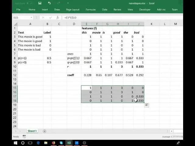
00:22:56.520 | Let's go back to our naive phase right in our naive phase

00:23:00.760 | We have this term document matrix, and then for every feature. We're calculating

00:23:06.960 | the probability of that feature occurring if it's class one that probability of that feature occurring if it's class two and then the

00:23:15.720 | ratio of those two

00:23:18.360 | Right and in the paper that we're actually lip basing this off. They call this P this Q and this

00:23:25.720 | Right, maybe I should just fill that in P

00:23:29.080 | Q maybe then we'll say probability to make it more obvious

00:23:35.920 | Okay

00:23:43.720 | And so then we kind of said hey, let's let's not use these ratios as the coefficients in that

00:23:50.520 | in that matrix multiply, but let's instead like

00:23:55.920 | Try and learn some coefficients. You know so maybe start out with some random numbers

00:24:00.520 | You know and then try and use stochastic gradient descent to find slightly better ones

00:24:09.880 | So you'll notice you know some important features here the the R

00:24:15.480 | Vector is a vector of rank 1 and its length is equal to the number of features

00:24:24.440 | and

00:24:25.760 | Of course our logistic regression coefficient matrix is also

00:24:30.560 | Of length 1 sorry rank 1 and length equal to the number of features right and we're you know

00:24:36.660 | We're saying like they're kind of two ways of calculating

00:24:38.680 | The same kind of thing right one based on theory one based on data

00:24:44.720 | So here is like some of the numbers in R right remember. It's using the log so these numbers

00:24:52.680 | Which are less than zero?

00:24:54.680 | represent things which are

00:24:57.120 | More likely to be negative and these ones that here are more likely

00:25:00.920 | Sorry this one here is more likely to be positive and so

00:25:04.700 | Here's e to the power of that and so these are the ones we can compare to one rather than to zero

00:25:10.720 | So I'm going to do something that hopefully is going to seem weird

00:25:20.520 | And so first of all I'm going to talk about I'm going to say what we're going to do and

00:25:25.120 | Then I'm going to try and describe why it's weird, and then we'll talk about

00:25:29.960 | Why it may not be as weird as we first thought so here's what we're going to do

00:25:34.320 | We're going to take our term document matrix

00:25:37.440 | And we're going to multiply it

00:25:40.160 | by R

00:25:43.160 | So what that means is we're going to we can do it here in Excel right so we're going to say

00:25:50.040 | let's grab everything in our term document matrix and

00:25:52.920 | Multiply it by the equivalent value in the vector of R. All right, so this is like a

00:25:58.880 | broadcasted element wise multiplication not a matrix multiplication

00:26:03.800 | Okay

00:26:08.280 | And that's what that does

00:26:13.320 | Okay, so here is the value of the term document matrix

00:26:20.020 | times R in other words everywhere that a zero appears there a zero appears here and

00:26:25.740 | Every time a one appears here the equivalent value of R appears here

00:26:30.820 | so we haven't really

00:26:33.540 | We haven't really changed much

00:26:37.140 | Right we've just we've just kind of

00:26:39.420 | Changed the ones into something else into the into the R's from that feature

00:26:45.020 | Right and so what we're now going to do is we're going to use this as

00:26:49.060 | our independent variables

00:26:51.980 | Instead in our logistic regression

00:26:54.260 | Okay, so here. We are multiply of X X NB X naive Bayes version is X times R

00:27:02.460 | And now let's do a logistic regression

00:27:04.940 | fitting using those independent variables and

00:27:08.740 | Let's then

00:27:13.500 | Do that for the validation set okay and get the predictions and

00:27:17.580 | Lo and behold we have a better number

00:27:21.420 | Okay, so

00:27:24.900 | Let me explain why this hopefully seems surprising

00:27:32.140 | Given that we're just multiplying oh

00:27:41.620 | I picked out the wrong ones. I should have said not coeth

00:27:46.180 | Okay, that's actually ah I got the wrong number okay

00:27:53.580 | So that's our independent variables right and then the the logistic regression has come up with some set of coefficients

00:28:02.460 | Let's pretend for a moment that these are the coefficients that it happened to come up with right

00:28:10.580 | We could now say well, let's not use this

00:28:13.980 | Set let's not use this

00:28:16.780 | Set of independent variables, but let's use the original binarized feature matrix right and then divide all of our coefficients

00:28:25.380 | by the values in R and

00:28:28.940 | We're going to get exactly

00:28:31.460 | the same result mathematically, so

00:28:35.020 | You know we've got

00:28:40.260 | X naive Bayes version of the independent variables, and we've got some

00:28:46.220 | Some set of weights some sort of some sort of coefficient so call it W

00:28:52.060 | right

00:28:55.220 | W 1 let's say

00:28:57.220 | Where it's found like this is a good set of coefficients and making our predictions from right, but X and B

00:29:04.820 | is simply equal to

00:29:07.740 | X

00:29:09.740 | times as in element wise times

00:29:12.460 | ah

00:29:15.100 | Right so in other words. This is equal to

00:29:17.720 | X times ah

00:29:22.540 | Times the weights and so like we could just change the weights to be that

00:29:30.220 | Right and get the same number

00:29:33.900 | so this ought to mean that

00:29:39.180 | The change that we made to the dependent variable shouldn't have made any difference

00:29:43.180 | Because we can calculate exactly the same thing without making that change

00:29:48.340 | So that's the question

00:29:51.700 | Why did it make a difference?

00:29:53.900 | So in order to answer this question

00:29:56.900 | I'm going to try and get you all to try and think about this in order to answer this question you need to think

00:30:00.900 | About like okay. What are the things that aren't?

00:30:05.620 | mathematically the same why is why is it not identical? What are the reasons like come up with some hypotheses? What are some reasons that maybe

00:30:12.300 | we've actually ended up with a

00:30:15.220 | Better answer and to figure that out. We need to first of all start with like well. Why is it even a different answer?

00:30:20.380 | Why is that different to that?

00:30:22.380 | This is subtle

00:30:32.460 | All right, what do you think I'm just wondering if it was two different kinds of multiplications

00:30:36.660 | You said that one is the element wise multiplication. No they did they do end up mathematically being the same, okay?

00:30:42.340 | Pretty much there's a minor wrinkle, but not but it's not that it's not some order operations thing

00:30:48.360 | Let's try can she

00:30:50.940 | You are on a roll today, so let's see how you go. I feel like the features are less

00:30:55.540 | correlated to each other I

00:30:59.780 | Mean I've made a claim that these are mathematically equivalent, so

00:31:04.900 | So what are you saying really you know why are we getting different answers?

00:31:11.340 | It's good people coming up with hypotheses. We need lots of wrong answers before we start finding. It's the right ones

00:31:21.460 | It's like that. You know I'm a warmer hotter colder. You know Ernest you're gonna get us hotter

00:31:25.540 | Does it have anything to do with the regularization? Yes, and is it the fact that when you so let's start there, right?

00:31:31.900 | So Ernest point here is like okay Jeremy. You've set their equivalent, but they're equivalent outcomes

00:31:37.820 | Right, but you got through you went through a process to get there and that process included regularization, and they're not necessarily equivalent

00:31:45.020 | Regularization like our loss function has a penalty so yeah help us think through and as how much that might impact things

00:31:52.820 | Well, this is maybe kind of dumb, but I'm just noticing that the numbers are bigger in the ones

00:31:57.940 | I've been weighted by the naive phase

00:31:59.940 | Mm-hmm are weights and so

00:32:02.660 | These are bigger and some are smaller some are bigger

00:32:06.420 | But that there are some bigger ones like the variance between the columns is much higher now the variance is bigger

00:32:11.460 | Yeah, I think that's a very interesting insight. Okay. That's all I got okay, so build on that

00:32:17.140 | I

00:32:19.140 | Prince has been on a roll a month so

00:32:24.900 | Hit us I'm not sure that's fine. Is it also considered like considering the dependency of different words?

00:32:31.740 | Is that why it is forming better rather than all?

00:32:35.300 | What independent of each other not really I mean it's it's you know again fear it

00:32:40.240 | You know theoretically these are creating mathematically equivalent outputs

00:32:45.540 | So they're not they're not doing something different except

00:32:50.300 | as Ernest mentioned

00:32:52.860 | They're getting

00:32:54.540 | impacted differently by regularization

00:32:56.540 | so what's

00:32:58.660 | So what's regularization right?

00:33:00.660 | regularization is we start out with our

00:33:04.220 | That was the weirdest thing I forgot to go into screenwriting mode, and it just turns out that you can actually write in Excel

00:33:13.020 | And I had no idea that was true

00:33:15.020 | I still use green writing rows, so I don't skill up my spreadsheet. I just I never tried

00:33:21.660 | So our loss was equal to like our cross entropy loss. You know based on the

00:33:31.240 | Predictions of the predictions and the actuals right plus our

00:33:43.220 | penalty

00:33:45.020 | so

00:33:47.020 | If you're

00:33:49.980 | If your weights a large

00:33:52.260 | Right then that piece

00:33:55.220 | Gets bigger

00:33:57.020 | Right and it drowns out that piece right, but that's actually the piece we care about right we actually want it to be a good fit

00:34:04.740 | So we want to have as little regularization going on as we can get away with we want so we want to have less

00:34:12.460 | weights

00:34:14.860 | So here's the thing right our value. Yes, can you pass it over here?

00:34:20.260 | We should let less weights do you mean lesser weights I do yeah

00:34:27.180 | Yeah, and I kind of use the two words a little equivalently, which is not quite fair

00:34:32.180 | I agree, but the idea is that weights that are pretty close to zero are kind of not there

00:34:35.740 | So here's the thing our values of are

00:34:42.460 | You know and I'm not a Bayesian weenie, but I'm still going to use the word prior right they're kind of like a prior

00:34:48.140 | so like we think

00:34:50.460 | that the

00:34:52.380 | The different levels of importance and positive or negative of these different features

00:34:58.220 | Might be something like that right we think that like bad

00:35:03.380 | you know might be

00:35:06.620 | More correlated with negative than

00:35:11.140 | Than good right so our kind of implicit assumption

00:35:16.500 | But before was that we have no priors so in other words when we'd said

00:35:23.500 | Squared weights we're saying a non zero weight is something. We don't want to have

00:35:28.780 | right, but actually I think what I really want to say is that

00:35:33.580 | Differing from the naive Bayes expectation is something. I don't want to do right

00:35:40.220 | Like only vary from the naive Bayes prior unless you have good reason to believe otherwise

00:35:46.780 | All right, and so that's actually what this ends up doing right we end up saying you know what?

00:35:53.860 | We think this value is probably three

00:35:58.060 | Right and so if you're going to like make it a lot bigger or a lot smaller

00:36:05.100 | Right that's going to create the kind of variation in weights. That's going to cause that squared term to go up right so

00:36:12.860 | so if you can

00:36:15.220 | You know just leave all these values about similar to where they are now

00:36:19.280 | Right and so that's what the penalty term is now doing right the penalty term when our inputs is already multiplied by R

00:36:26.980 | Is saying penalize things where we're varying it from our naive Bayes

00:36:34.060 | prior

00:36:36.060 | Can you pass that

00:36:38.540 | Why multiply only with the R not

00:36:42.780 | Constant like R squared or something like that when the variance would be much higher this time

00:36:47.520 | because our

00:36:50.580 | Our prior comes from an actual theoretical model right so I said like I don't like to rely on theory

00:36:58.220 | But I have if I have some theory

00:37:01.580 | Then you know maybe we should use that as our starting point rather than starting off by assuming everything's equal

00:37:08.060 | So our prior said hey, we've got this model called naive Bayes and the naive Bayes model said

00:37:13.700 | If the naive Bayes assumptions were correct

00:37:17.140 | Then R is the correct coefficient right in this specific

00:37:22.500 | formulation

00:37:24.580 | That that's why we pick that because our our prior is based on that that theory

00:37:29.940 | Okay, so this is a really interesting insight, which I

00:37:39.180 | Never really see covered which is this idea is that we can use these like, you know traditional

00:37:47.500 | Machine learning techniques we can imbue them with this kind of Bayesian sense

00:37:53.140 | by by starting out

00:37:57.500 | You know incorporating our theoretical expectations

00:38:01.180 | Into the data that we give our model right and when we do so

00:38:06.220 | that then means

00:38:08.540 | We don't have to regularize as much and that's good right because if we regularize a lot

00:38:13.380 | But let's try it

00:38:16.300 | Let's go back to

00:38:19.580 | You know here's our

00:38:22.500 | Our

00:38:24.500 | Remember the way they do it in the sklearn logistic regression is this is the reciprocal of the amount of

00:38:35.900 | regularization penalty, so we'll kind of

00:38:39.660 | Add lots of regularization by making it small

00:38:44.660 | So that's like really hurts

00:38:51.580 | That really hurts our accuracy because now

00:38:54.100 | It's trying really hard to get those weights down. The loss function is overwhelmed

00:38:59.540 | By the need to reduce the weights and the need to make it predictive is kind of now seems totally unimportant

00:39:08.060 | right, so

00:39:10.660 | So by kind of starting out and saying you know what don't push the weights down so that you end up

00:39:17.540 | ignoring

00:39:20.020 | The the terms but instead push them down so that you try to get rid of you know ignore

00:39:26.020 | differences from our

00:39:28.700 | expectation based on the naive phase

00:39:30.700 | formulation

00:39:33.140 | So that

00:39:37.340 | Ends up giving us a

00:39:40.540 | very nice

00:39:42.860 | Result which actually was originally this this technique was originally presented. I think about 2012

00:39:49.380 | Chris Manning who's a terrific NLP researcher up at Stanford and

00:39:53.480 | Cedar Wang who I don't know but I assume is awesome because this paper is awesome. They basically came up

00:39:59.340 | with this with this idea and

00:40:02.520 | What they did was they compared it to a number of other approaches on a number of other

00:40:11.300 | Datasets so one of the things they tried is this one is the IMDB data set right and so here's naive Bayes SVM on bigrams

00:40:18.220 | And as you can see this approach out performed the other

00:40:23.060 | linear based approaches that they looked at and also some

00:40:27.140 | Restricted Boltzmann machine kind of neural net based approaches. They looked at now nowadays

00:40:34.700 | There are better ways there

00:40:36.700 | You know there are better ways to do this and in fact in the deep learning course

00:40:39.580 | We showed a new state-of-the-art result that we just developed at fast AI that gets

00:40:43.380 | Well over 94%

00:40:46.180 | But still you know like particularly for a linear technique. That's easy fast and intuitive

00:40:52.460 | This is pretty good

00:40:53.180 | And you'll notice when they when they did this they only used by grams

00:40:57.540 | And I assume that's because they I looked at their code, and it was kind of pretty slow and ugly

00:41:02.180 | You know I figured out a way to optimize it a lot more as you saw and so we were able to use

00:41:08.300 | Here trigrams, and so we get quite a lot better

00:41:12.500 | So we've got 91.8 versus in 91.2, but other than that it's identical

00:41:16.820 | Also, I mean they used a support vector machine. Which is almost identical to a logistic aggression in this case

00:41:24.900 | So there's some minor differences right so I think that's a pretty cool result and

00:41:32.220 | You know I will mention

00:41:36.780 | You know what you get to see here in class is the result of like

00:41:41.460 | many

00:41:43.340 | Weeks and often many months of research that I do and so I don't want you to think like this stuff is obvious

00:41:49.940 | It's not at all like reading this paper

00:41:51.940 | There's no description in the paper of like

00:41:55.800 | Why they use this model how it's different why they thought it works?

00:42:00.900 | You know it took me a week or two to even realize that it's kind of like mathematically equivalent

00:42:06.660 | To a normal logistic regression and then a few more weeks to realize that the difference is actually in the regularization

00:42:12.620 | You know like this is kind of like

00:42:16.620 | Machine learning as I'm sure you've noticed from the Kaggle competitions you enter you know like you come up with a thousand good ideas

00:42:24.140 | 999 of them no matter how confident you are they're going to be great

00:42:28.380 | They always turn out to be shit

00:42:29.500 | you know and then finally after four weeks one of them finally works and

00:42:34.540 | Kind of gives you the enthusiasm to spend another four weeks of misery and frustration

00:42:39.900 | This is the norm right and and like

00:42:43.820 | For sure that the best

00:42:47.580 | Practition as I know in machine learning all share one particular trait in common, which is they're very very tenacious

00:42:55.500 | You know also known as stubborn and bloody-minded right which is definitely a reputation. I seem to have

00:43:03.420 | probably fair

00:43:05.420 | Along with another thing which is that they're all very good coders. You know they're very good at turning their ideas into into code

00:43:12.620 | So yeah

00:43:16.020 | So you know this was like a really interesting

00:43:18.020 | Experience for me working through this a few months ago to try and like figure out how to how to at least

00:43:24.260 | You know how to explain why this at the at the time kind of state-of-the-art result exists

00:43:30.780 | And so once I figured that out. I was actually able to build on top of it and make it quite a bit better

00:43:37.060 | And I'll show you what I did and this is where it was very very handy to have high torch at my disposal

00:43:44.880 | Because I was able to kind of create something that was

00:43:48.700 | Customized just the way that I wanted to be and also very fast by using the GPU

00:43:56.100 | So here's the kind of fast AI version of the NB SVM actually my friend Stephen Marity. Who's a

00:44:03.460 | terrific

00:44:05.980 | Researcher in NLP has christened this the NB SVM plus plus which I thought was lovely

00:44:11.980 | So here is the even though there is no SVM. It's a logistic regression, but as I said nearly exactly the same thing

00:44:17.540 | So let me first of all show you like the code

00:44:22.180 | So this is like we try to like once I figure out like okay

00:44:25.180 | This is like the best way I can come up with to do a linear bag-of-words model

00:44:28.860 | I kind of embed it into fast AI so you can just write a couple of lines of code

00:44:32.180 | So the code is basically hey, I want to create a data class for text classification

00:44:37.860 | I want to create it from a bag of words

00:44:40.080 | Right here is my bag of words

00:44:42.740 | Here are my labels

00:44:45.020 | Here is the same thing for the validation set

00:44:48.060 | and use up to

00:44:51.860 | 2,000 unique words per review which is plenty

00:44:56.440 | So then from that model data

00:45:01.780 | Construct a a learner which is kind of the fast AI generalization of a model

00:45:07.380 | Which is based on a dot product of naive Bayes and then fit that model

00:45:13.400 | And then do a few epochs and

00:45:18.100 | After five epochs I was already up to ninety two point two. All right, so this is now like, you know getting

00:45:25.060 | quite well above

00:45:27.300 | this this linear baseline

00:45:29.300 | So, let me show you the code for for that

00:45:34.200 | So the code is like

00:45:42.580 | horrifyingly short

00:45:44.580 | That's it. Right and it'll also look on the whole

00:45:48.700 | Extremely familiar, right? There's if there's a few tweaks here

00:45:52.780 | Pretend this thing that says embedding pretend it actually says linear. Okay, I'm going to show you embedding in a moment

00:45:58.700 | Pretend it says linear

00:45:59.420 | So we've got basically a linear layer where the number of features coming with the number of features as the rows and remember

00:46:06.500 | SK learn features means number of words basically and then for each row we're going to create

00:46:13.420 | One weight which makes sense right for like a logistic regression every every so not for each row for each word

00:46:21.060 | each word has one weight and

00:46:23.860 | Then we're going to be multiplying it by the the R values. So for each word

00:46:31.440 | We have one R value per class. So I actually made this so this can handle like not just

00:46:38.500 | Positive versus negative but maybe figuring out like which author created this work. There could be five or six authors

00:46:44.740 | Whatever right and basically we kind of use those linear layers

00:46:49.740 | to to get the

00:46:53.140 | The value of the weight and the value of the R and then we take the weight

00:46:58.500 | times the R and

00:47:02.140 | Then sum it up. And so that's just a dot product. Okay, so just just a simple dot product just as we would do for any

00:47:09.660 | logistic regression

00:47:11.660 | And then do the softmax

00:47:13.660 | So the very minor tweak

00:47:18.140 | That we add to get the the better result is this the main one really is this here this plus something

00:47:26.780 | right the thing I'm adding is

00:47:30.020 | It's a parameter, but I pretty much always use this this version this value 0.4

00:47:34.220 | So what does this do?

00:47:36.980 | So what this is doing is it's again kind of changing the prior, right? So if you think about it

00:47:44.620 | Even once we use this R times the term document matrix as our independent variables

00:47:56.460 | You really want to start with a question? Okay, the penalty terms are still pushing W down to zero, right?

00:48:03.180 | So what did it mean?

00:48:05.180 | For W to be 0 right? So what would it mean if we had you know?

00:48:10.460 | Coefficient 0 0 0 0 0

00:48:14.460 | Right. So what that would do when we go? Okay this matrix times these coefficients

00:48:22.340 | We still get 0

00:48:24.540 | Right. So a weight of 0 still ends up saying I have no opinion on whether this thing is positive or negative

00:48:30.580 | On the other hand if they were all 1

00:48:35.220 | Right, then it's basically says my opinion is that the naive phase coefficients are exactly right

00:48:45.500 | Okay, and so the idea is that I said

00:48:52.780 | 0 is almost certainly not

00:48:54.980 | The right prior right we shouldn't really be saying if there's no coefficient. It means ignore the naive Bayes coefficient

00:49:02.320 | One is probably too high

00:49:05.380 | Right because we actually think that naive Bayes is only kind of part of the answer

00:49:09.860 | All right, and so I played around with a few different data sets where I basically said

00:49:15.020 | Take the weights and add to them

00:49:21.900 | some constant

00:49:23.900 | Right, and so 0 would become in this case 0.4

00:49:29.300 | right, so in other words the

00:49:31.900 | the regularization

00:49:35.060 | Penalty is pushing the weights not towards 0 but towards this value

00:49:41.180 | Right, and I found that across a number of data sets 0.4

00:49:46.100 | Works pretty well that and it's pretty resilient. All right. So again, this is the basic idea is to kind of like

00:49:53.660 | Get the best of both worlds, you know, we're we're we're learning from the data using a simple model

00:50:00.780 | But we're incorporating

00:50:03.580 | You know our prior knowledge as best as we can and so it turns out when you say, okay

00:50:10.120 | Let's let's tell it, you know as weight matrix of zeros

00:50:15.620 | Actually means that you should use about you know about half of the R values

00:50:20.140 | That ends up that ends up working better than the prior that the weights should all be zero

00:50:28.620 | Yes

00:50:31.700 | Is the the weights the W is it that the point for the amount of regularization required?

00:50:39.140 | the amount of so we have this

00:50:43.780 | term where the we have the term where we reduce the amount of error the prediction error RMSE plus we have the

00:50:51.140 | Regularization and is it W the point for denote the amount of realization required? So W are the weights

00:50:57.460 | Right, so this is calculating our activations. Okay, so we calculate our activations as being equal to the weights

00:51:06.020 | Times the R

00:51:12.060 | Sum all right, so that's just our normal

00:51:15.680 | At a normal linear function, right so so the the thing which is being penalized is

00:51:26.740 | my weight matrix

00:51:29.580 | That's what gets penalized

00:51:31.580 | So by saying hey, you know what don't just use W use W plus point four

00:51:36.460 | So that's not being penalized

00:51:39.180 | It's not part of the weight matrix

00:51:41.860 | Okay, so effectively the weight matrix gets 0.4 for free

00:51:47.340 | So by doing this

00:51:52.780 | even after regularization then

00:51:55.460 | every

00:51:57.420 | Absolutely

00:51:58.500 | Every feature is getting some form of weight some form of minimum weight or something like that

00:52:03.340 | Um, not necessarily because it could end up choosing a coefficient of negative point four for a feature

00:52:09.300 | And so that would say

00:52:11.300 | You know what even though naive Bayes says it's the R should be whatever for this feature. I think you should totally ignore it

00:52:18.980 | Yeah

00:52:20.660 | great questions, okay

00:52:22.660 | We started at 20 past

00:52:29.440 | - okay, let's take a break for about eight minutes or so and start back about 25 to

00:52:37.820 | four

00:52:39.820 | Okay, so a couple of questions at the break the first was just for a

00:52:51.300 | Kind of

00:52:55.220 | Reminder or a bit of a summary as to what's going on

00:52:58.500 | Yeah, right. And so here we have

00:53:02.660 | W plus

00:53:06.180 | I'm writing it out. Yeah plus

00:53:11.500 | Adjusted weight a weight adjustment times

00:53:17.020 | Right, so so normally what we were doing

00:53:22.580 | So normally what we were doing is saying hey logistic regression is basically

00:53:30.380 | Wx right. I'm going to ignore the bias

00:53:34.420 | Okay, and then we were changing it to be

00:53:37.500 | W dot

00:53:40.460 | Times x

00:53:42.940 | Right, and then we were kind of saying let's do that bit first

00:53:48.380 | right

00:53:51.220 | Although in this particular case actually now I look at it. I'm doing it in this code. It doesn't matter obviously in this code

00:53:58.620 | I'm actually doing

00:54:00.620 | I'm

00:54:02.620 | Doing this bit first

00:54:07.460 | And so

00:54:11.100 | So this thing here actually I could I called it W which is probably pretty bad. It's actually W times X

00:54:24.740 | Right, so so instead of W times X times R. I've got W times X

00:54:33.260 | plus a

00:54:36.020 | constant times R

00:54:38.020 | right

00:54:39.700 | So the the key idea here is

00:54:42.540 | that

00:54:44.780 | regularization

00:54:46.780 | Can't draw in yellow that's fair enough

00:54:54.020 | Regularization wants the weights to be zero right because we're trying to it's trying to reduce

00:55:02.180 | That okay, and

00:55:05.980 | so what we're saying is like okay, we want to push the weights towards zero because we're saying like that's our like

00:55:13.780 | default starting point expectation is the weights are zero and

00:55:19.300 | So we want to be in a situation where if the weights is zero, then we have a model that like

00:55:25.380 | Makes theoretical or intuitive sense to us, right?

00:55:30.660 | This model if the weights are zero doesn't make intuitive sense to us

00:55:36.820 | Right because it's saying hey multiply everything by zero gets rid of all of that and gets rid of that as well

00:55:42.860 | And we were actually saying no we actually think our our is useful. We actually want to keep that

00:55:49.060 | right, so

00:55:51.060 | So instead we say you know what let's take that piece here and add

00:55:58.260 | Zero point four to it

00:56:01.980 | Right so now if the regularizer is pushing the weights towards zero

00:56:06.740 | Then it's pushing the value of this sum

00:56:10.100 | towards zero point four

00:56:12.660 | Right and so therefore it's pushing our whole model to zero point four times up

00:56:19.100 | Right so in other words

00:56:21.100 | Now kind of default starting point if you've regularized all the weights out all together is to say yeah

00:56:27.380 | You know let's use a bit of our that's probably a good idea

00:56:30.420 | Okay

00:56:34.100 | So that's the idea right that's the idea is basically you know what happens when

00:56:40.020 | When that's zero right and you and you want that to like be something sensible because otherwise

00:56:48.460 | Regularizing the weights to move in that direction wouldn't be such a good idea

00:56:53.040 | Second question was about

00:56:59.340 | N grams

00:57:05.500 | So the N in N gram can be uni by try whatever one two three whatever grounds so for the this movie is good

00:57:15.340 | All right, it has four unigrams this movie is good

00:57:23.660 | It has three bigrams this movie movie is is good

00:57:30.700 | It has two trigrams

00:57:33.620 | This movie is

00:57:35.900 | Movie is good

00:57:38.260 | Okay

00:57:42.060 | Can you pass that? So yeah, do you mind go back to the wad chase down the zero point four stuff?

00:57:50.180 | yeah, so I was wondering if this adjustment will harm the predictability of the model because

00:57:56.420 | Think of extreme extreme case if it's not zero point four if it's four thousand and or

00:58:03.660 | Coefficient will be like right essentially. So so exactly so so our prior

00:58:09.540 | Needs to make sense and so our prior here and you know

00:58:13.060 | This is why it's called dot prod MB is our prior is that this is something where we think naive Bayes is a good prior

00:58:20.660 | Right and so naive Bayes says that are equals

00:58:25.220 | P over

00:58:28.180 | That's not how you write P P over Q. I have not had much sleep

00:58:33.620 | P over Q is a good prior and not only do we think it's a good prior

00:58:38.420 | But we think our

00:58:40.420 | Times X plus B is a good model

00:58:46.500 | That's that's the naive Bayes model. So in other words, we expect that

00:58:51.620 | You know a coefficient of one is a good coefficient not not four thousand

00:58:58.600 | Yeah, so we think specifically we don't think we think zero is probably not a good coefficient

00:59:05.540 | All right, but we also think that maybe

00:59:08.100 | The naive Bayes version is a little overconfident. So maybe one's a little high

00:59:13.260 | So we're pretty sure that the right number assuming that our model a naive Bayes model is as appropriate is between

00:59:20.500 | zero and one

00:59:23.140 | No, but what I was thinking is as long as it's not zero you are pushing those

00:59:31.380 | Coefficients that are supposed to be zero to something not zero and makes the

00:59:35.720 | Like high coefficients less distinctive from the mode coefficients

00:59:41.100 | Well, but you see they're not supposed to be zero. They're supposed to be our

00:59:45.460 | Mike that's that's what they're supposed to be. They're supposed to be our right and so

00:59:52.380 | and remember

00:59:54.540 | This is inside our forward function

00:59:56.780 | So this is part of what we're taking the gradient of right? So it's basically

01:00:01.660 | Saying okay, we're still gonna you know, you can still set

01:00:05.460 | self dot W to anything you like

01:00:08.500 | But just the regularizer

01:00:12.260 | Wants it to be zero and so all we're saying is okay if you want it to be zero then I'll try to make zero be

01:00:20.340 | You know give a sensible answer

01:00:24.260 | That's the basic idea and like yeah, nothing says point four is perfect for every data set

01:00:29.460 | I've tried a few different data sets and found various numbers between point three and point six that are optimal

01:00:34.980 | But I've never found one where point four is

01:00:38.180 | Less good than zero which is not surprising and I've also never found one where one is better, right?

01:00:45.100 | So the idea is like this is a reasonable default, but it's another parameter you can play with which I kind of like right?

01:00:50.020 | It's another thing you could

01:00:51.620 | use

01:00:53.180 | Grid search or whatever to figure out for your data set. What's best and you know really the key here being

01:00:59.020 | Every model before this one as far as I know has implicitly assumed

01:01:05.420 | It should be zero because they just they don't have this parameter right and you know by the way

01:01:10.100 | I've actually got a second parameter here as well

01:01:12.100 | Which is the same thing I do to our is actually divide our

01:01:15.940 | By a parameter

01:01:18.180 | Which I'm not going to worry too much about it now

01:01:20.380 | But again, it's this is another parameter you can use to kind of adjust what the nature of the regularization is

01:01:25.660 | You know and I mean in the end I'm I'm a

01:01:29.460 | Empiricist not a theoretician. You know that I thought this seemed like a good idea

01:01:33.420 | Nearly all of my things it seemed like a good idea turn out to be stupid this particular one

01:01:38.740 | Dave good results, you know on this data set and a few other ones as well

01:01:43.740 | Okay, could you pass that?

01:01:47.540 | Yeah, I'm sure a little bit confused about the W plus W adjusted. Uh-huh

01:01:52.240 | So you mentioned that we do W plus W adjusted so that the coefficients don't get set to zero

01:02:00.100 | that we place some importance on the priors, but you also said that the

01:02:05.420 | Effect of learning can be that W gets set to a negative value which in fact really does W plus W

01:02:12.020 | Right zero. So if if we are we are allowing the learning process to indeed set the priors to zero

01:02:20.020 | So why is that in any way different from just having W because yeah, great question because of regularization because we're panelizing it by that

01:02:30.340 | Right so in other words

01:02:33.980 | We're saying you know what if you if the best thing to do is to ignore the value of R

01:02:40.620 | That'll cost you you're going to have to set W to a negative number

01:02:44.220 | Right so only do that if that's clearly a good idea unless it's clearly a good idea then you should leave

01:02:53.420 | Leave it where it is

01:02:56.340 | That's that's the only reason like all of this stuff. We've done today is basically entirely about

01:03:02.840 | You know maximizing the advantage we get from regularization and saying regularization

01:03:09.020 | pushes us towards some default assumption and nearly all of the machine learning literature assumes that default assumption is

01:03:17.100 | Everything zero and I'm saying like it turns out

01:03:21.120 | You know it makes sense theoretically and turns out empirically that actually you should decide what your default assumption is

01:03:27.900 | And that'll give you better results. So would it be right to say that?

01:03:32.940 | In a way, you're putting an additional hurdle in the along the way towards getting all coefficients to zero

01:03:39.500 | So it will be able to do that if it is really worth it

01:03:42.940 | Yeah, exactly. So I'd say like the default hurdle without this is is

01:03:46.940 | Making a coefficient non zero is the hook hurdle and now I'm saying no the co-op that the hurdle is making a coefficient

01:03:54.220 | Not be equal to point four R

01:04:02.500 | So this is sum of W square into C

01:04:06.840 | Some of it is some lambda or C penalty constant

01:04:12.400 | Yeah, yeah time something. Yeah, so the weight decay should also depend on the value of C if it is very less

01:04:18.940 | Like if C is right by say, do you mean this?

01:04:22.020 | Hey, yeah. Yeah. So if a is point one, then the weights might not go

01:04:29.220 | Towards you then we might not need great decay. So well that the whatever this value

01:04:35.140 | I mean if the if the value of this is zero, then there is no recurization, right?

01:04:39.180 | But if this value is higher than zero then there is some penalty

01:04:43.660 | right and and presumably we've set it to non zero because we're overfitting so we want some penalty and so if there is some penalty then

01:04:54.340 | Then my assertion is that we should penalize things that are different to our prior

01:04:59.980 | Not that we should penalize things that are different to zero

01:05:03.020 | And our prior is that things should be you know around about equal to our

01:05:11.700 | Okay, let's move on thanks for the great questions, I want to talk about

01:05:23.860 | Embedding I

01:05:25.660 | Said pretend. It's linear and indeed we can pretend. It's linear

01:05:29.140 | Let me show you how much we can pretend. It's linear as in nn dot linear create a linear layer

01:05:33.980 | Here is our

01:05:37.300 | Data matrix

01:05:39.500 | All right, here are our coefficients if we're doing the our vision here our coefficients are

01:05:44.460 | right, so if we were to

01:05:47.940 | Put those into a column vector

01:05:53.980 | like

01:05:55.980 | So right then we could do a matrix multiply of that

01:06:01.620 | By that right and so we're going to end up with

01:06:07.960 | So here's our matrix is our vector

01:06:21.300 | Alright, so we're going to end up with

01:06:23.300 | One times one plus one times one one times one one times three

01:06:31.020 | Right zero times one zero times point three

01:06:41.320 | All right, and then the next one zero times one one times one so forth okay, so like that the matrix multiply

01:06:50.300 | you know of

01:06:52.300 | this independent

01:06:54.300 | Variable matrix

01:06:57.220 | By this coefficient matrix is going to give us an answer okay, so that's that is just a matrix multiply

01:07:03.860 | So the question is like okay. Well. Why didn't Jeremy right and n dot linear? Why did Jeremy right and n dot embedding?

01:07:12.100 | And the reason is because if you recall we don't actually store it like this

01:07:19.300 | Because this is actually of width

01:07:21.300 | 800,000 and

01:07:23.740 | of height

01:07:25.620 | 25,000 right so rather than storing it like this

01:07:29.220 | we actually store it as

01:07:32.300 | Zero one two three right one two three four zero one two

01:07:43.620 | five

01:07:46.860 | One two four five

01:07:48.860 | Okay

01:07:52.620 | That's actually how we store it that is this bag of words contains which word indexes

01:08:01.940 | That makes sense

01:08:05.060 | okay, so that's like

01:08:07.060 | This is like a sparse way of

01:08:11.220 | Of storing it right is just list out the indexes in each sentence

01:08:16.940 | So given that I

01:08:20.420 | Want to now do that matrix multiply that I just showed you to create that same

01:08:26.940 | outcome

01:08:29.020 | Right, but I want to do it from this representation

01:08:32.300 | So if you think about it

01:08:36.020 | All this is actually doing is

01:08:40.420 | It's saying a one hot you know this is basically one hot encoded right?

01:08:46.020 | It's kind of like a dummy dummy matrix version does it have the word this does it have the word movie?

01:08:50.980 | Does it have the word is and so forth?

01:08:53.100 | So if we took the simple version of like does it have the word this one?

01:08:58.300 | Right and we multiplied that

01:09:04.420 | By that

01:09:08.380 | Right then that's just going to return the first item

01:09:12.900 | That makes sense

01:09:16.500 | So in general a

01:09:19.780 | One hot encoded

01:09:22.900 | vector

01:09:24.740 | times a matrix is

01:09:26.740 | Identical to to looking up that matrix to find the nth row in it

01:09:34.100 | Right so this is identical to saying find the zero first second and fifth

01:09:39.300 | coefficients

01:09:42.460 | Right so they're they're the same they're exactly the same thing and like it doesn't like in this case. I only have one

01:09:49.660 | Coefficient per feature right but actually the way I did this was to have

01:09:55.660 | One coefficient per feature for each class

01:10:01.780 | Right so in this case is both positive and negative

01:10:04.260 | So I actually had kind of like an R positive and an R negative

01:10:09.460 | So negative would be just the opposite right equals that

01:10:13.340 | Divided by that right now the binary case obviously it's redundant to have both, but what if it was like?

01:10:21.420 | What's the author of this text is it?

01:10:26.980 | Jeremy or Savannah or Terrence right now. We've got three categories. We want three

01:10:32.580 | Values of R right so the nice thing is then this sparse version

01:10:38.380 | You know you can just look up. You know the zeroth and the first and the second and the fifth

01:10:46.580 | Right and again, it's identical

01:10:49.100 | mathematically identical

01:10:51.900 | to multiplying by a one hot encoded matrix

01:10:54.180 | but

01:10:56.260 | When you have sparse inputs, it's obviously much much more efficient

01:11:02.120 | so this

01:11:05.180 | computational trick

01:11:07.900 | Which is mathematically identical to not conceptually analogous to mathematically identical to

01:11:14.040 | Multiplying by a one hot encoded matrix is called an embedding

01:11:18.260 | Right, so I'm sure you've all heard or most of you probably heard about embeddings like word embeddings word to back or glove

01:11:26.060 | or whatever and

01:11:28.060 | People love to make them sound like there's some

01:11:30.700 | Amazing you complex neural net thing right they're not

01:11:36.860 | embedding means

01:11:39.420 | Make a multiplication by a one hot encoded matrix faster by replacing it with a simple array look up

01:11:46.300 | Okay, so that's why I said

01:11:49.260 | You can think of this as if it said self dot W equals n n dot linear

01:11:55.540 | and

01:11:56.540 | F plus 1 by 1 right because it actually does

01:12:00.260 | The same thing right it actually is a matrix with those dimensions. This actually is a matrix with those dimensions

01:12:08.300 | All right, it's a linear layer

01:12:10.300 | But it's expecting that the input we're going to give it is not actually a one hot encoded matrix

01:12:18.900 | But it's actually a list of integers

01:12:21.580 | right the indexes for each

01:12:24.580 | Word or for each item so you can see that the forward function in fast AI

01:12:30.180 | Automatically gets for this learner

01:12:33.060 | the feature indexes right so they come from

01:12:37.300 | The sparse matrix automatically numpy makes it very easy to just grab those those indexes

01:12:44.340 | Okay, so in other words there. We've got here. We've got a list of

01:12:51.180 | each word index of a of the 800,000 that are in this document and

01:12:55.980 | So then this here says look up each of those in our embedding matrix

01:13:02.260 | Which is got 800,000 rows and return

01:13:05.420 | Each thing that you find

01:13:08.180 | Okay

01:13:10.260 | so mathematically identical to

01:13:13.460 | multiplying by the one hot encoded matrix

01:13:18.820 | That makes sense, so that's all an embedding is and so what that means is

01:13:25.260 | We can now handle

01:13:31.860 | Building any kind of model like a you know whatever kind of neural network

01:13:37.140 | Where we have potentially very high cardinality categorical variables as our inputs

01:13:45.300 | We can then just turn them into a numeric code between zero and the number of levels and

01:13:51.380 | then we can learn a

01:13:54.660 | You know a

01:13:57.900 | Linear layer from that as if we had one hot encoded it

01:14:02.000 | Without ever actually constructing the one hot encoded version

01:14:06.180 | And without ever actually doing that matrix multiply okay instead. We will just store

01:14:12.460 | The index version and simply do the array lookup

01:14:16.100 | Okay, and so the gradients that are flowing back

01:14:19.580 | You know basically in the one hot encoded version everything that was a zero has no gradient

01:14:24.500 | So the gradients flowing back is best go to update the particular row of the embedding matrix that we used

01:14:31.500 | okay, and so

01:14:33.900 | That's fundamentally important for NLP

01:14:37.700 | Just like here like you know I wanted to create

01:14:41.460 | a pie torch model that would implement this

01:14:45.700 | this ridiculously simple little equation right and

01:14:50.300 | To do it without this trick would have meant I was beating in a 25,000 by that hatred the 800,000

01:14:58.620 | element array

01:15:01.620 | Which would have been kind of crazy right and so this this trick allowed me to write you know

01:15:07.340 | You know I just replaced the word linear with embedding

01:15:10.740 | replace the thing that feeds the

01:15:12.740 | One hot encodings in with something that just feeds the indexes in and that was it that that it kept working

01:15:18.020 | And so this now trains

01:15:20.020 | You know in about a minute per epoch

01:15:24.860 | Okay

01:15:30.620 | so

01:15:32.380 | What we can now do is we can now take this idea and apply it not just to language

01:15:38.940 | But to anything right for example

01:15:41.460 | Predicting the sales of items at a grocery

01:15:46.460 | Yes, where's the

01:15:50.340 | Just a quick question so we are not actually looking up anything right

01:15:56.540 | We are just saying that now that array with the indices that is the representation

01:16:01.060 | So the represent so we are doing a lookup right the representation

01:16:06.020 | That's being stored it for the but for the bag of words is now not

01:16:09.780 | 1 1 1 0 0 1 but 0 1 2 5 right and so then

01:16:15.980 | We actually have to do our

01:16:18.660 | Matrix product right but rather than doing the matrix product we look up

01:16:23.160 | The zeroth thing and the first thing and the second thing and the fifth thing

01:16:29.220 | So that means we are still retaining the one hot encoded matrix no

01:16:35.740 | We didn't there's no one-hot encoded matrix used here. This is the one-hot encoded matrix, which is not currently highlighted

01:16:41.860 | We've currently highlighted the list of indexes and the list of coefficients from the weight matrix

01:16:50.700 | That makes sense

01:16:54.140 | Okay

01:16:57.460 | So what we're going to do now is we're kind of going to go to go a step further and saying like

01:17:03.180 | Let's not use a linear model at all

01:17:05.180 | Let's use a multi-layer neural network, right and let's have the input to that potentially be

01:17:11.900 | Include some categorical variables right and those categorical variables. We will just have as

01:17:18.300 | Numeric indexes

01:17:22.420 | And so the first layer for those won't be a normal linear layer. There'll be an embedding layer

01:17:27.420 | Which we know behaves exactly like a linear layer

01:17:32.100 | mathematically

01:17:33.220 | And so then I hope will be that we can now use this to create a neural network for any kind of data

01:17:39.380 | right and so

01:17:42.020 | There was a competition on

01:17:45.980 | Kaggle a few years ago called Rossman, which is a German grocery chain

01:17:52.140 | Where they asked to predict the sales of items in?

01:17:58.220 | their stores right and that included the mixture of categorical and continuous variables and

01:18:03.740 | In this paper by Gwar and Birkin they described their third place winning entry

01:18:08.500 | Which was much simpler than the first place winning entry

01:18:14.020 | But nearly as good

01:18:16.980 | But much much simpler because they took advantage of this idea of what they call entity embeddings

01:18:24.580 | in the paper they they thought I think that they had invented this actually had been written before earlier by

01:18:31.100 | Yoshio Benjio and his co-authors in another Kaggle competition, which was predicting taxi destinations

01:18:36.980 | although I will say I feel like

01:18:39.900 | Gore went a lot further in describing how this can be

01:18:45.020 | Used in many other ways

01:18:47.620 | And so we'll talk about that as well

01:18:53.340 | So

01:18:54.980 | the

01:18:56.980 | So this one is actually in the is in the deep learning one repo. Okay deal one

01:19:02.780 | Lesson three, okay

01:19:05.540 | Because we talk about some of the deep learning specific aspects in the deep learning course where else in this course

01:19:10.300 | We're going to be talking mainly about the feature engineering

01:19:13.180 | And we're also going to be talking about you know kind of this this embedding idea

01:19:19.860 | So

01:19:21.860 | Let's start with the data right so the data was you know store number one on the 31st of July 2015

01:19:33.100 | was open

01:19:35.980 | They had a promotion going on

01:19:37.980 | It was a school holiday. It was not a state holiday, and they sold five thousand two hundred and sixty three items

01:19:44.660 | So

01:19:48.180 | That's the key

01:19:49.820 | Data they provided and so the goal is obviously to predict sales in a test set that has the same information without sales

01:19:57.500 | They also tell you that for each store

01:20:02.500 | It's of some particular type

01:20:05.460 | It sells some particular assortment of goods

01:20:08.740 | Its nearest competitor competitor is some distance away

01:20:12.860 | The competitor opened in September 2008

01:20:17.980 | And there's some more information about promos. I don't know the details of what that means

01:20:22.660 | Like in many Kaggle competitions they let you

01:20:28.740 | download

01:20:30.860 | External data sets if you wish as long as you share them with other competitors

01:20:34.860 | So people oh they also told you what state each store is in so people downloaded a list of the names of the different states

01:20:42.540 | of Germany

01:20:43.820 | They downloaded a file for each state in Germany for each week

01:20:48.580 | Some kind of Google trend data. I don't know what specific Google trend they got but there was that

01:20:55.060 | For each date they downloaded a whole bunch of temperature information

01:20:58.860 | That's it, and then here's the test set

01:21:04.460 | okay, so I

01:21:06.940 | Mean one interesting insight here

01:21:08.780 | Is that there was probably a mistake in some ways for Rossman to design this competition as being one where you could use external data?

01:21:15.980 | Because in reality you don't actually get to find out next week's weather or next week's Google trends

01:21:22.300 | You know

01:21:23.940 | But you know when you're competing in Kaggle you don't care about that you just want to win

01:21:28.140 | So you use whatever you can get?

01:21:35.900 | So let's talk first of all about data cleaning you know that there wasn't really much feature engineering done in this third place

01:21:42.660 | Winning entry like bite bite particularly by Kaggle standards where normally every last thing counts

01:21:50.620 | This is a great example of how far you can get with with a neural net and it certainly reminds me of the

01:21:57.460 | claims prediction competition we talked about yesterday where the winner did no feature engineering and entirely relied on deep learning

01:22:05.540 | the

01:22:07.540 | Laughter in the room I guess is from people who did a little bit more than no feature engineering in that competition

01:22:15.840 | So you know I should mention by the way like I

01:22:20.620 | find that bit where like you work hard at a competition and then it closes and

01:22:26.620 | You didn't win and the winner comes out and says this is how I won like that's the bit where you learn the most right?

01:22:34.020 | But sometimes that's happened to me, and it's been like oh

01:22:37.700 | I've thought of that

01:22:39.860 | I thought I tried that and then I go back and I realize I like had a bug there

01:22:45.540 | I didn't test properly and I learned like okay like I really need to learn to like test this thing in this different way

01:22:52.180 | Sometimes it's like oh, I thought of that, but I assumed it wouldn't work

01:22:56.980 | I've really got to remember to check everything before I make any assumptions

01:23:00.980 | And you know sometimes it's just like oh, I did not think of that technique

01:23:06.220 | Wow now I know it's better than everything

01:23:09.460 | I just tried because like otherwise somebody says like hey you know here's a really good technique

01:23:14.300 | You're like okay great right, but when you spent months trying to do something and like somebody else did it better by using that technique

01:23:22.460 | That's pretty convincing

01:23:24.380 | Right and so like it's kind of hard like I'm standing up in front of you saying

01:23:28.460 | Here's a bunch of techniques that I've I've used and I've won some Kaggle competitions

01:23:33.420 | And I've got some state-of-the-art results, but it's like that's kind of second-hand information by the time it hits you right, so it's really great to

01:23:40.660 | Yeah, try things out and and also like it's been kind of nice to see

01:23:46.020 | Particularly I've noticed in the deep learning course quite a few of my students have you know

01:23:50.860 | I've said like this technique works really well

01:23:52.780 | And they've tried it and they've got into the top ten of a Kaggle competition the next day, and they're like

01:23:57.980 | Okay, that that counts is working really well, so so yeah Kaggle competitions are

01:24:03.040 | Helpful for lots and lots of reasons

01:24:06.340 | But you know one of the best ways is what happens after it finishes and so definitely like

01:24:10.460 | For the ones that you that are now finishing up make sure you you know watch the forums

01:24:15.060 | See what people are sharing in terms of their solutions

01:24:18.520 | And you know if you want to learn more about them like feel free to ask

01:24:24.260 | The winners like hey, could you tell me more about this so that people are normally pretty pretty good about explaining

01:24:29.500 | And then ideally try and replicate it yourself, right and that can turn into a great blog post

01:24:36.580 | You know or a great colonel is to be able to say okay such-and-such said that they use this technique

01:24:42.320 | Here's a really short explanation of what that technique is and here's a little bit of code showing how it's implemented

01:24:48.140 | And you know here's the result showing you you can get the same result that can be a really interesting write-up as well

01:24:53.900 | Okay, so

01:24:55.900 | You know it's it's always nice to kind of have your data reflect

01:25:03.280 | Like I don't know be as kind of easy to understand as possible

01:25:10.380 | So in this case the data that came from Kaggle used various you know integers for the holidays

01:25:15.780 | We can just use a boolean of like was it a holiday or not?

01:25:19.180 | So like just clean that up

01:25:23.260 | We've got quite a few different tables. We need to join them all together

01:25:26.500 | Right I have a standard way of joining things together with pandas

01:25:31.700 | I just use the pandas merge function and specifically I always do a left joint

01:25:37.580 | So who wants to tell me what a left join is?

01:25:41.460 | Since it's there once go ahead

01:25:44.740 | So you retain all the rows in the left table and you take so you have a key column

01:25:50.780 | You match that with the key column in the right side table, and you just merge the rows that are also present in the right side

01:25:56.620 | Yeah, that's a great explanation good job. I don't have much to add to that thick the key reason that I always do a left

01:26:01.980 | join is

01:26:03.780 | That after I do the join. I always then check if there were things in the right hand side

01:26:10.420 | That are now null right because if so it means that I missed some things

01:26:15.520 | I haven't shown it here, but I also check that the number of rows

01:26:20.220 | Hasn't varied before and after if it has that means that the right hand side table wasn't

01:26:25.740 | Unique okay, so

01:26:28.300 | Even when I'm sure something's true. I always also assume that I've screwed it up, so I always check

01:26:36.500 | So I could go ahead and merge the state names into the weather I can also

01:26:43.140 | If you look at the

01:26:47.100 | Google Trends table

01:26:52.100 | It's got this weak range which I need to turn into a date in order to join it

01:26:57.840 | Right and so the nice thing about doing this in pandas is that pandas gives us access to you know all of Python

01:27:05.360 | Right and so for example inside the the series object is a dot str

01:27:11.940 | Attribute that gives you access to all the string processing functions

01:27:15.900 | Not just like cat gives you access to the categorical functions

01:27:19.140 | DT gives you access to the daytime functions so I can now split

01:27:23.140 | Everything in that column, and it's really important to try and use these pandas functions

01:27:27.460 | Because they you know they're going to be vectorized accelerated through you know often through CMD at least through you know C code

01:27:35.740 | So that runs nice and quickly

01:27:39.600 | and

01:27:42.220 | Then you know as per usual let's add date metadata to our dates

01:27:47.460 | In the end we are basically denormalizing all these tables, so we're going to put them all into one table so in the Google trend

01:27:57.780 | table

01:27:59.900 | There was also though they were mainly trends by state, but there was also trends for the whole of Germany

01:28:06.260 | So we kind of put the Germany own you know the whole of Germany ones into a separate data frame so that we can join that

01:28:12.780 | So we're going to have like Google trend for this date and Google trend for the whole of Germany

01:28:17.640 | And so now we can go ahead and start joining

01:28:21.740 | Both for the training set and for the test set and then for both checks that we don't have zeros

01:28:27.740 | My merge function

01:28:33.660 | I set the suffix if there are two columns that are the same I set the suffix on the left to be nothing at all

01:28:39.840 | So it doesn't screw around with the name and the right hand side to be underscore Y and in this case

01:28:45.140 | I didn't want any of the duplicate ones, so I just went through and

01:28:48.980 | Deleted them okay

01:28:52.820 | And then we're gonna in a moment. We're going to try to

01:28:59.220 | Create a competition you know the the main competitor for this store has been open since some date

01:29:05.960 | Right and so you can just use pandas to date time passing in the year the month and the day

01:29:13.780 | Right and so that's going to give us an error unless they all have years and months

01:29:19.060 | So so we're going to fill in the missing ones with the 1900 and a 1

01:29:23.700 | Okay, and then what we really know it we didn't want to know is like how long is this store been open for?

01:29:29.620 | At the time of this particular record all right, so we can just do a date subtract, okay?

01:29:35.740 | Now if you think about it sometimes the competition

01:29:41.900 | You know opened later than this particular row so sometimes it's going to be negative and it doesn't probably make sense

01:29:50.940 | To have negative spending like it's going to open in x days time now having said that I would never

01:29:58.540 | Put in something like this

01:30:01.740 | Without first of all running a model with it in and without it in right because like our assumptions about

01:30:09.820 | About the data very often turn out not to be true now in this case. I didn't invent any of these

01:30:18.180 | pre-processing steps I wrote all the code, but it's all based on the third place winners github repo, right so

01:30:26.580 | Knowing what it takes to get third place in the Kaggle competition

01:30:31.060 | I'm pretty sure they would have checked every one of these pre-processing steps and made sure it actually improved there

01:30:36.860 | their validation set score

01:30:39.380 | Okay

01:30:42.020 | So what we're going to be doing is

01:30:47.180 | creating a neural network where some of the inputs to it are

01:30:53.020 | continuous and some of them are categorical and

01:30:57.700 | So what that means in the in the neural net that you know we have

01:31:03.220 | We're basically going to have you know this kind of initial weight matrix right and we're going to have this

01:31:16.940 | This input feature vector right and so some of the inputs are just going to be plain

01:31:22.660 | Continuous numbers like you know what's the maximum temperature here, or what's the number of plumbers to the nearest store?

01:31:29.140 | And some of them are going to be

01:31:32.660 | One hot encoded

01:31:38.220 | Effectively right, but we're not actually going to store it as one hot encoded

01:31:44.180 | We're actually going to store it as

01:31:46.180 | the index

01:31:48.180 | Right and so the neural net model is going to need to know which of these columns

01:31:53.900 | Should you should you basically create an embedding for which ones should you treat?

01:31:58.460 | You know as if they were kind of one hot encoded and which ones should you just feed directly into the linear layer?

01:32:05.740 | right and so

01:32:08.340 | We're going to tell the model when we get there

01:32:10.540 | Which is which but we actually need to think ahead of time about like which ones?

01:32:15.020 | Do we want to treat as categorical and which ones are continuous in particular?

01:32:20.260 | Things that we're going to treat it as categorical

01:32:22.780 | We don't want to create

01:32:25.140 | More categories than we need all right, and so let me show you what I mean

01:32:28.780 | the

01:32:31.740 | The the third place getters in this competition

01:32:34.140 | Decided that the number of months that the competition was open was something that they were going to use as a categorical variable

01:32:40.300 | Right and so in order to avoid having more categories than they needed

01:32:44.240 | They truncated it at 24 months. They said anything more than 24 months. I'll truncate to 24

01:32:51.180 | So here are the unique values of competition months open, and it's all the numbers from naught to 24

01:32:57.120 | right

01:32:59.620 | So what that means is that there's going to be you know an embedding matrix

01:33:04.500 | That's going to have basically an embedding vector for things that aren't open yet for things that are open a month

01:33:10.820 | So things that are open two months and so forth now

01:33:13.740 | They absolutely could have done that as a

01:33:17.020 | Continuous variable right they could have just had a number here

01:33:21.380 | Which is just a single number of how many months has it been open?

01:33:24.260 | And they could have treated it as continuous and fed it straight into the initial weight matrix

01:33:30.860 | what I found though and obviously what these competitors found is

01:33:35.900 | Where possible it's best to treat things as categorical variables

01:33:41.620 | All right

01:33:44.380 | And the reason for that is that like when you feed something through an embedding matrix?

01:33:50.140 | You basically mean it means every level can be treated like totally differently

01:33:55.940 | Right and so for example in this case whether something's been open for zero months or one month is

01:34:02.620 | Right really different right and so if you fed that in as a continuous variable

01:34:07.940 | It would be kind of difficult for the neural net to try and find a functional form that kind of has that that big difference

01:34:14.820 | It's possible because neural nets can do anything right, but you're not making it easy for it

01:34:18.740 | Where else if you used an embedding treated it as categorical then it'll have a totally different vector for zero versus one

01:34:25.380 | Right so it seems like particularly as long as you've got enough data

01:34:29.360 | that

01:34:31.820 | The treating columns as categorical variables where possible is a better idea

01:34:36.620 | And so I say when I say where possible that kind of basically means like

01:34:41.340 | Where the cardinality is not too high

01:34:44.900 | You know so if this was like

01:34:47.980 | You know

01:34:51.620 | The sales ID number that was like uniquely different on every row

01:34:55.440 | You can't treat that as a categorical variable

01:34:58.260 | Right because you know it would be a huge embedding matrix and everything only appears once or ditto for like

01:35:05.420 | kilometers away from the nearest store

01:35:07.780 | To two decimal places you wouldn't make a categorical variable, right?

01:35:12.300 | So that's kind of the that's kind of the rule of thumb

01:35:16.900 | That they both used in this competition in fact if we scroll down

01:35:21.260 | to their choices

01:35:23.260 | Here is how they did it right they're continuous variables with things that were genuinely

01:35:30.380 | Continuous like number of kilometers away to the competitor the temperature stuff

01:35:35.340 | Right the number you know the specific number in the Google trend, right?

01:35:41.020 | Where else everything else basically they treat it as categorical

01:35:49.380 | Okay, so that's it for today, so yeah next time. We'll

01:35:55.100 | We'll finish this off. We'll see we'll see how to turn this into a neural network

01:35:59.740 | and

01:36:02.780 | Yeah, kind of wrap things up so see you then

Machine Learning 1: Lesson 11

Chapters