HNSW for Vector Search Explained and Implemented with Faiss (Python)

00:00:00.000 | Hi and welcome to the video. We're going to be having a look at the Hierarchical Navigable Small

00:00:06.080 | Worlds graph or HNSW graph and how it's used in vector search. Now HNSW is one of the best

00:00:17.520 | performing algorithms for approximate nearest neighbors search and what I want to do with this

00:00:25.520 | video is explore how it works and how we can implement it in FICE. So let's go ahead and get

00:00:35.200 | started. Now we'll start with the sort of foundations of HNSW and where it comes from.

00:00:46.800 | So we can split approximate nearest neighbor algorithms into three broad categories. Trees,

00:00:54.960 | hashes, and graphs. Now HNSW, it was HNSW graph so we can figure out it probably belongs in the

00:01:02.800 | graph category and more specifically it's a type of proximity graph which is it simply

00:01:09.600 | means that vertices which are just the vectors in our graph or the nodes in our graph

00:01:16.720 | are connected to other nodes or vertices based on their proximity and we would typically

00:01:24.160 | measure this proximity using Euclidean distance. We don't have to but that's the sort of standard.

00:01:32.720 | Now going from a proximity graph which is pretty simple to a HNSW graph is a pretty big leap

00:01:42.880 | and there's two main algorithms that have really helped me understand what HNSW actually does and

00:01:52.880 | that is the probability skip list and the navigable small world graphs which are just

00:01:58.800 | the predecessors of HNSW. So what I'm going to do is just quickly you know run through those

00:02:07.680 | two algorithms. So this is a probability skip list. It's reasonably old. It was introduced in

00:02:15.840 | 1990 by a guy called William Poog and it works by building several layers of linked list which

00:02:23.520 | is what you can see up here. So what we do with this is we we're looking for the number 11 or the

00:02:30.400 | key 11 and we saw over here the top layer of our start block and what we do is we say in our layer

00:02:40.320 | 3 which is our entry layer and we move across. So we go over to the next block here and we say okay

00:02:48.800 | number 11 is not 5 and 5 is not greater than 11. So we continue and we go all the way over to the

00:02:57.360 | end block over here. Once we reach the end block we know that we need to go to the next layer so

00:03:05.280 | one layer down and so we do that we go to layer 2 at the start block again and we continue moving

00:03:14.480 | across. Now at this point we get to block 19 over here and we say okay 19 is a great 11 so now we

00:03:23.760 | know that we need to go on to our next layer, layer 1 down here and then we go across and we

00:03:30.640 | find number 11. Now the whole point of this is when we have a lot of values this can reduce the

00:03:39.600 | number of steps we need to take in order to get to our final value rather than just going along

00:03:46.000 | our layer 0 and going along every single value within our list. HNSW borrows this hierarchical

00:03:57.360 | layered format or levels as we will see pretty soon. Navigable Small World or NSW graphs were

00:04:05.600 | developed over the course of a few papers around 2011 up to 2014. The basic idea is that we can

00:04:15.920 | have a very large graph with many vertices and because we have both short range links so the

00:04:27.440 | sort of links that you see on the outside of our circle here and we also have these long range

00:04:33.600 | links which is what you see going across the circle we make our graph very navigable so it's

00:04:40.480 | very easy to get from one point to another in very few steps and there's some terminology that we

00:04:47.600 | should cover here which is the all the vertices we have here all of their connections so all the

00:04:54.640 | other vertices that they are connected to we refer to these as that vertex's friends list okay and

00:05:04.160 | when searching this NSW graph we begin at a predetermined entry point so in here we see

00:05:11.440 | we're sort of sawing a few different points but in reality with these sort of big graphs we always

00:05:18.160 | start with one specific entry point or maybe sometimes we can do use different entry points

00:05:25.440 | based on some sort of logic but we have either one or if only a few entry points in our graph

00:05:34.320 | and then what we do is we perform what is called greedy routing now routing just refers to the

00:05:43.520 | route that we take through our graph and greedy refers to the fact that we are always going to

00:05:49.360 | choose out of our vertices friend list we're going to choose the friend that is the closest to our

00:05:59.040 | target vertex now if we find that there are no near vertices in our friend list this is a local

00:06:09.760 | minimum and this is our stopping condition we cannot get any closer we're kind of stuck in

00:06:16.400 | in that local minimum now if our vertex has very few friends we can get stuck

00:06:24.320 | quite easily so we can get stuck in the local minimum if there are less connections

00:06:28.960 | and we actually refer to vertices that have

00:06:40.080 | fewer friends as a low degree vertex so it's low degree it means it has a low number of links or

00:06:48.160 | edges and then we also have high degree vertices now with these it's if we are currently on a high

00:06:57.440 | degree vertex it's harder to get stuck in local minimum because we have more options on where we

00:07:02.480 | can where we can move now the routing through a navigable small world graph is split into two

00:07:09.520 | phases so we have the typically the earlier zoom out phase where we are passing through vertices

00:07:18.720 | that have a low number of links and then we also have the zoom in phase where we are passing through

00:07:28.320 | high degree vertices which have a lot of links and what we tend to find is a high degree vertices

00:07:35.280 | will usually have more long range links so we can move further across our graph with these

00:07:42.160 | high degree vertices now to minimize the probability of stopping early so avoiding

00:07:49.120 | those local minima we can increase the average degree of our vertices now this also increases

00:07:59.520 | the complexity of our network and therefore slows down our search time so we have to find a balance

00:08:07.360 | between both of those now another approach to avoiding hitting a local minima too early

00:08:14.800 | is to start search on high degree vertices so the vertices which have a lot of connections now

00:08:22.960 | for nsw we can do this and it works it works for low dimensional data but it doesn't work perfectly

00:08:32.400 | and it's actually one of the key factors that hnsw improves upon and uses to improve its own

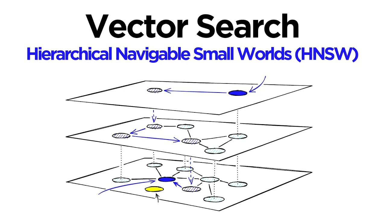
00:08:40.560 | performance so let's move on to to hsw and how both this fit into hsw so hsw is obviously a

00:08:50.480 | an evolution of nsw and it borrows inspiration from poops probability skip list structure with

00:08:59.280 | the with the hierarchy so you can you can see that here we have a few different layers so we

00:09:04.720 | have our entry layer just like we did with the probability skip list structure and we also have

00:09:12.160 | an entry point and what we've basically done here is taken a navigable small nsw graph and split it

00:09:20.720 | across multiple layers so high vertex high degree vertices will tend to be spread across more layers

00:09:32.400 | because when we're building our graph we add the number of friends based on which layer it gets

00:09:41.520 | inserted at the higher the layer that the vertex is inserted at the more friends it's going to have

00:09:48.480 | which makes a high degree vertex and what that does is if we start at that highest layer that

00:09:55.360 | means we're on high degree vertices so we are less likely to get stuck in the local minimum

00:10:01.520 | and that means we're not going to stop early so that allows us to start the top layer and we move

00:10:08.080 | through our graph and what we do is we have our query vector and on each layer we

00:10:17.200 | keep moving or traversing across different edges in that layer in essentially the same way we did

00:10:25.280 | for an sw so we greedily identify the friend of our current vertex that has the least distance

00:10:34.560 | from our query vector and we move to that and then we we keep doing that and once we hit a local

00:10:42.640 | minimum we we don't stop the whole thing we just move down to the next layer and then we we do it

00:10:50.720 | again and we keep doing that until we reach the local minimum of layer zero and that is our

00:10:58.800 | stopping condition that's where we stop now that that's how we search that's what our graph looks

00:11:03.840 | like and how we search but let's have a quick look at how we actually build that graph so

00:11:09.360 | what we do is we have a probability function which essentially says we're pretty much going

00:11:19.040 | to put every vertex or every vector on layer zero not every but a pretty high number of them as we'll

00:11:26.880 | see later and we say okay we get a uniform a random number from uniform distribution

00:11:35.360 | and if that number is greater than our probability for that level we move on to

00:11:42.720 | the next layer so we increment our layer so let's say this turns out to not be true we move up a

00:11:53.280 | layer and we we try again okay now this next layer is going to have lower probability but we're also

00:11:59.920 | going to subtract the probability value from our lower layer from the random number that we've

00:12:08.400 | produced and we keep doing this again and again until we get up to our top layer at that point

00:12:15.200 | there are no other layers this is very unlikely to happen if we say if we have a billion maybe

00:12:23.280 | not a billion like a hundred i think it was a hundred million vectors i tried this with

00:12:28.400 | i got i think four vectors on the top layer so it is it's very unlikely for one vector to go all the

00:12:36.640 | way up to the top but if it does we insert it at that layer and it has the possibility of becoming

00:12:43.600 | a entry point for our graph one other thing that we we also have here is the the ml at the top

00:12:50.480 | now this is called the level multiplier and this value is it's just a normalization value

00:12:59.600 | which allows us to modify the probability or the probability distribution across each one of our

00:13:06.400 | layers now the the creators of hsw they found that the the best value for ml the optimum value

00:13:16.320 | was to use one over the natural logarithm of m and m we'll we'll have a look at that pretty soon

00:13:25.520 | that's just the number of neighbors each vertex is assigned so here we have we we have m so we've set

00:13:33.760 | m to three and we we're saying here so we want to insert this blue vector so that blue vector you

00:13:44.720 | see we've decided okay we're going to insert at layer one that means it gets an insert of it both

00:13:51.520 | layer one and layer zero but not at layer two and we we go through our graph just like we do when we

00:14:01.920 | search but this time we're we're trying to find many neighbors of our new vertex that we can assign

00:14:11.280 | to it's friendless and what we have here is so with an m value of three we would add three neighbors

00:14:22.400 | to that vertex both on layer one and also on layer zero now we can also have a m m max value and an

00:14:32.640 | m max zero value which is what we have down here and basically as more vertices are added we may

00:14:46.000 | find that this vertex ends up with more than three friends and maybe that that's fine but

00:14:55.280 | what we essentially do is use m max to say okay if we have any vertices with more than this number

00:15:03.280 | of friends we need to trim it and we need to just keep the closest like three in this example

00:15:10.400 | and then m max zero is another value and that is the same so it's the maximum number of friends

00:15:17.760 | of vertex you have but for layer zero which is i think always a higher number than the other layers

00:15:25.600 | now one other thing that we we should cover very quickly is we also have two more variables ef

00:15:33.200 | construction ef search now ef construction is used on we're building our graph and it's basically

00:15:40.400 | the number of friends of our inserted vertex that we will use when traversing across layers so in

00:15:50.800 | layer one up here we we have these three friends and that means that during our search for

00:15:57.840 | friends in the low layers we would go down like this we would start our search from each of these

00:16:06.720 | three vertices in the lower layer okay now that would be the case for all of those

00:16:16.000 | and ef search is the same but it's used during search time to search through our graph

00:16:21.360 | and i mean that they're pretty much that's pretty much all we need to know

00:16:27.520 | in on the theory side of hsw so let's dive into the implementation of hsw in advice

00:16:39.680 | okay so in we're in python now all i've done is taken our data so i'm using the sift 1m data set

00:16:47.440 | as we as we usually do and all i'm going to do is use this to you know search throughout our index

00:16:55.440 | as always now the first thing we want to do is actually create or initialize our index so i'm

00:17:02.400 | going to use two parameters so we have d which is the dimensionality the sift 1m data set so the

00:17:09.200 | length of our vectors in there and also m now m if you remember that's the number of neighbors

00:17:16.880 | that we will assign to each vertex in our graph now for this i'm going to use a value of 32

00:17:24.080 | and what we can now do is we write index equals advice

00:17:34.000 | index flat hsw and then we just passed dnm and that's you know we've initialized

00:17:43.360 | okay sorry so it's not flat hsw it's hsw flat okay there we go so with that we have initialized our

00:17:59.120 | index of course there's nothing in there at the moment and we can see that so we can go ahead and

00:18:06.240 | write index hsw max level to see okay how many levels do we have in our index and we'll see that

00:18:16.560 | we get this minus one which means that the the level is in there that the structure has not

00:18:22.800 | been initialized yet and we also see that if we we do this so this is how we get the

00:18:29.840 | number of vertices that we have within each layer so we write the vice vector to array

00:18:40.000 | and in here we want to write index hsw levels and then let's print out

00:18:52.160 | and we see that we we just get this empty array now what we'd also want to do when we do so this

00:18:58.160 | is just a massive array so if we we will have a million values in here once we we add our cif-1m

00:19:09.040 | data set so what we do is we just write npb count levels to count the number to count basically how

00:19:18.960 | many vertices we have in each level when i say level by the way it's the same as earlier on when

00:19:25.440 | i was saying layers it's they're the same so when i say levels layers same thing so obviously at the

00:19:33.840 | moment we don't have anything in our graph so how do we how do we add that we we already know

00:19:41.600 | we just do index add xb okay nothing else so we add that that might take some time because

00:19:50.560 | we're building the graph we saw before it's a reasonably intensive process so it does take a

00:19:55.680 | little bit of time i think maybe around 40 seconds for this so i will fast forward okay so it's done

00:20:06.000 | 52 seconds not too bad now what we're now going to do is i want to have a look at these again so

00:20:14.240 | let's see if we we have a structure in our graph yet so max level so that's cool we have that means

00:20:21.440 | we have five levels zero one two up to four and then if we do this again we'll be able to see the

00:20:30.320 | distribution of vertices across each one of those levels so i'll just write this there we go so we

00:20:38.880 | just ignore this this first one here that doesn't mean anything so this is our layer zero like i

00:20:46.400 | said most vectors get assigned to this layer now we have layer one all the way up to layer four here

00:20:56.320 | or level four now vice will always add at least one vertex to your maximum level because

00:21:05.680 | otherwise we we don't have an entry point to our graph so there's always at least one in there

00:21:11.120 | and we can also check what which vector is being used there so we can write index hsw

00:21:20.880 | entry points yes and there we have said that that's the number of our vector that we have added

00:21:31.120 | as our entry point up here you can also change that if you want but i wouldn't probably especially

00:21:37.840 | with this i definitely wouldn't recommend it now i was super curious as to how it decides

00:21:43.920 | where to insert everything so went through the code which you can find over here so this is the

00:21:52.240 | defy scale repo and we have this hsw cpp file and in here we come down and it might take me a little

00:22:02.320 | while so this is where we initialize our index and we have this set default probus so if we if we go

00:22:11.680 | into set default progress we will find this here which is not really too hard to read i don't

00:22:20.080 | read i don't know c++ but this is pretty simple and what i translated that to in python is this

00:22:28.720 | here with a few comments because there is no comments in the other file for some reason

00:22:35.360 | now what we're basically doing is just building a probability distribution for each of our layers

00:22:42.560 | and we do using this this function here so we're taking the exponential of the the level

00:22:51.280 | divided by at that ml function or value that i mentioned earlier so that's the the multi-level

00:22:59.920 | the level multiplier value and what we get is a probability for the current level now

00:23:07.840 | what we do is once we reach a particularly low probability we we start creating new levels

00:23:15.840 | so if we we run this oh another actually interesting thing is here we we are saying

00:23:25.440 | on every level we will assign m neighbors as our as our m max except from level zero

00:23:32.720 | where we will assign two m okay so this is this m times like two so for our use case we had 32

00:23:44.000 | we had m set to 32 so that means in all of our layers except from layer zero we'll have

00:23:50.480 | each vertex will have 32 neighbors or friends and on layer or level zero it will have 64

00:23:59.760 | friends so i thought that was that was also interesting so

00:24:03.440 | we can go ahead and run that so i'm the 32 here is our m we can replace it m if you if we want

00:24:13.600 | so we run that and we get this probability distribution so this is for layer zero the

00:24:19.520 | probability of it being added using a random number generator so we're saying if our randomly

00:24:26.160 | generated number is less than this value we will assign or we will insert our vertex on at level

00:24:35.600 | zero and then we continue that logic all the way down to here which is our level four and then here

00:24:43.600 | is the total number so the cumulative number of neighbors per level so if we insert at level four

00:24:50.400 | we we will have this many neighbors for that vertex in total if we insert level zero we have 64 again

00:24:58.320 | a little bit interesting now in the in the code we when we're inserting vertices we use another

00:25:07.200 | function this is the last one we're not going to go through all of them we're just going to go

00:25:10.800 | through this one we insert or we decide where to insert our vertex using this function here which

00:25:17.040 | is the random level function this takes our sign probus from up here so this here and also a

00:25:25.840 | randomly generated number so here i'm using the numpy's random number generator

00:25:33.840 | and we go through and that's that's how we assign a different level for each of our values so if i

00:25:42.000 | let's run that and we'll see that we get a very similar distribution to to what we get in vice

00:25:52.240 | which i is i think pretty cool to see so if we do the bin count again we get this now if you take a

00:26:01.760 | look at this these values are so close to to what we produce up here so where is it um so here look

00:26:12.720 | at these values almost exactly the same so yeah it's pretty close they're both working in the same

00:26:23.520 | way now i also visualize that in in this chart here so you can you can see okay on the right

00:26:33.280 | we have a python version on the left we have our vice version and i've included the numbers in there

00:26:38.720 | basically that is exactly it's pretty much exactly the same it's off by a few here and there but not

00:26:45.280 | much so i thought that was pretty cool to see now okay that's cool that's how everything works

00:26:53.280 | that's interesting but what i think many of us are probably most interested in is how do i build the

00:27:02.400 | best hs sub u index for my for my use case for what i want so i ran some codes to go through

00:27:12.240 | all of that and pretty much i did this so we have this is also a good thing for me to show you um

00:27:22.960 | is how we get out ef construction and ef search values so i think you know a good starting point

00:27:29.760 | for both of these values is probably 16 32 is reasonable but you can play around them i think

00:27:40.800 | that's usually the best way and for most of what i'm going to show you i was using this so i was

00:27:47.600 | performing a thousand queries and calculating the recall at one value for those also i was

00:27:57.040 | checking you know how long our search is taking and the memory usage of each of these indexes

00:28:02.960 | so the first thing i wanted to look at is a recall of course so in in what what we have here

00:28:13.840 | on the left we have with a ef constriction value of two which is is very low i person i

00:28:21.200 | i don't know never use that never use an ef constriction value that low it well well you

00:28:28.000 | can see the recall is pretty terrible but you know surprisingly even though this is a very bad

00:28:33.200 | ef constriction value still got up to 40 percent recall so i was impressed with that that was cool

00:28:42.240 | and so the ef search values are what you can see on the bottom so it went from from i think two all

00:28:48.320 | the way up to 256 256 yeah that's right and we did that again for the ef constriction value of 16 here

00:28:59.200 | and also 64 i did it for more ef constriction values but these are probably the ones i think

00:29:05.440 | showed the relationship best and then all the colors you can see here we have a few different

00:29:10.560 | colors we're using different m values so what i found from this is that you basically you want

00:29:19.760 | to increase your your m and your ef search values to improve your recall and ef construction also

00:29:26.960 | helps with that so higher ef constriction value means that we need lower ef search and m values

00:29:33.440 | to achieve you know the same the same recall now of course you know we can just increase all of

00:29:40.960 | these and we we get better recall but that isn't for free we have to sacrifice some of our search

00:29:50.560 | time as well as always so we well this is this is what we've got so same same graphs as last time

00:30:01.040 | this time we have search time on the y-axis now ef construction here

00:30:07.760 | does actually make a bit of a difference when we start using higher m values so i found before in

00:30:18.000 | previous videos and articles that ef construction didn't really have too much of an effect

00:30:23.200 | on the search time which seemed fair enough because it is mostly a index construction

00:30:31.120 | parameter but that it does seem to have some effect when you start adding or increasing

00:30:38.000 | the number of queries that you are searching for and in particular where you have high m values

00:30:45.040 | now one thing to also note here is that we're using a load scale on the y-axis so

00:30:52.000 | the the higher values are definitely a fair bit higher but again i mean if we if we go for a sort

00:30:59.280 | of reasonable ef search value all of these are pretty high i mean 256 for your search values

00:31:05.840 | is high if we go for sort of es search of 32 let's say around here

00:31:18.800 | we're still getting reasonable search times so this is on the

00:31:21.920 | millisecond well it's a bit more than a millisecond scale

00:31:25.840 | and if we if we take a look at that on uh recall we're sort of getting up into the sort of 60

00:31:38.320 | 60 plus area at that point six cent plus and and look obviously it's not bad it's reasonably good

00:31:48.400 | but you can you can definitely get better than that when you start merging different

00:31:52.720 | indexes which we have covered all of that in another video another article so you'll be

00:32:01.120 | able to find that in in the either at the bottom of the article if you're reading the article

00:32:05.600 | or in the the video description if you're watching us on youtube

00:32:08.960 | now having a look at the the ef construction values again their effect on the search time

00:32:16.720 | we find that ef construction when we use those lower end values like i mentioned it doesn't

00:32:22.720 | have too much of a impact on the search time so if you are using a lower m value i think ef

00:32:29.520 | construction is a a good value to increase because it doesn't tend to make push up your search time

00:32:37.680 | too much and you can improve your recall fair bit by increasing it so it's definitely one to

00:32:46.080 | one to try and increase them and see how it goes for me i found it it's been quite useful at least

00:32:52.000 | and then finally the sort of negative point of h and sub u is the memory usage is just

00:33:00.640 | through the roof as you can see here so using the lowest m value which i think was

00:33:06.160 | two which is you you would never ever use that we were getting a memory usage for the sift 1m

00:33:13.120 | data set of more than more than half a gigabyte if you push m up a lot i mean 500 and 512 is is

00:33:23.600 | maybe a little bit too much but we're sort of pushing four and a half gigabytes five gigabytes

00:33:29.680 | so it's something to be aware of i think but like i said before we can we can still improve the the

00:33:39.840 | memory usage and the search speed by simply using different indexes alongside our hsw index so

00:33:47.760 | if memory usage is a concern you just compress the vectors using product quantization

00:33:52.960 | if the speed if you need it to be even faster you can use the an ibf index on top of hsw to improve

00:34:05.120 | the search times and if you want both of those you just put them all together and you can get

00:34:11.280 | that as well now like i said we we have covered all that in a lot more detail in another article

00:34:18.160 | and video but for this video on hsw i think now we're gonna leave it there i think we've covered

00:34:28.160 | plenty so thank you very much for watching and i'll see you in the next one bye

HNSW for Vector Search Explained and Implemented with Faiss (Python)

Chapters