The spelled-out intro to language modeling: building makemore

00:00:00.000 | Hi everyone, hope you're well.

00:00:02.480 | And next up what I'd like to do is I'd like to build out Makemore.

00:00:06.320 | Like micrograd before it, Makemore is a repository that I have on my GitHub web page.

00:00:11.440 | You can look at it.

00:00:12.760 | But just like with micrograd, I'm going to build it out step by step, and I'm going to

00:00:16.600 | spell everything out.

00:00:17.920 | So we're going to build it out slowly and together.

00:00:20.400 | Now what is Makemore?

00:00:22.000 | Makemore, as the name suggests, makes more of things that you give it.

00:00:27.800 | So here's an example.

00:00:29.320 | Names.txt is an example dataset to Makemore.

00:00:32.800 | And when you look at names.txt, you'll find that it's a very large dataset of names.

00:00:38.360 | So here's lots of different types of names.

00:00:41.800 | In fact, I believe there are 32,000 names that I've sort of found randomly on a government

00:00:46.520 | website.

00:00:48.120 | And if you train Makemore on this dataset, it will learn to make more of things like

00:00:53.360 | this.

00:00:54.360 | And in particular, in this case, that will mean more things that sound name-like, but

00:01:00.600 | are actually unique names.

00:01:02.560 | And maybe if you have a baby and you're trying to assign a name, maybe you're looking for

00:01:05.680 | a cool new sounding unique name, Makemore might help you.

00:01:09.780 | So here are some example generations from the neural network once we train it on our

00:01:14.720 | dataset.

00:01:16.440 | So here's some example unique names that it will generate.

00:01:20.000 | So, "Montel", "Irat", "Zendi", and so on.

00:01:25.840 | And so all these sort of sound name-like, but they're not, of course, names.

00:01:30.900 | So under the hood, Makemore is a character-level language model.

00:01:34.980 | So what that means is that it is treating every single line here as an example.

00:01:39.880 | And within each example, it's treating them all as sequences of individual characters.

00:01:45.260 | So R-E-E-S-E is this example.

00:01:49.160 | And that's the sequence of characters.

00:01:50.800 | And that's the level on which we are building out Makemore.

00:01:54.160 | And what it means to be a character-level language model then is that it's just sort

00:01:58.440 | of modeling those sequences of characters, and it knows how to predict the next character

00:02:02.000 | in the sequence.

00:02:03.840 | Now we're actually going to implement a large number of character-level language models

00:02:08.160 | in terms of the neural networks that are involved in predicting the next character in a sequence.

00:02:12.520 | So very simple bigram and bag-of-word models, multilayered perceptrons, recurrent neural

00:02:17.720 | networks, all the way to modern transformers.

00:02:19.840 | In fact, the transformer that we will build will be basically the equivalent transformer

00:02:24.880 | to GPT-2, if you have heard of GPT.

00:02:28.280 | So that's kind of a big deal.

00:02:29.480 | It's a modern network.

00:02:30.840 | And by the end of the series, you will actually understand how that works on the level of

00:02:35.000 | characters.

00:02:36.000 | Now, to give you a sense of the extensions here, after characters, we will probably spend

00:02:41.280 | some time on the word level so that we can generate documents of words, not just little

00:02:45.640 | segments of characters, but we can generate entire large, much larger documents.

00:02:51.280 | And then we're probably going to go into images and image-text networks, such as DALI, stable

00:02:56.600 | diffusion, and so on.

00:02:58.360 | But for now, we have to start here, character-level language modeling.

00:03:02.520 | Let's go.

00:03:03.660 | So like before, we are starting with a completely blank Jupyter Notebook page.

00:03:07.240 | The first thing is I would like to basically load up the dataset, names.txt.

00:03:12.040 | So we're going to open up names.txt for reading, and we're going to read in everything into

00:03:17.680 | a massive string.

00:03:20.060 | And then because it's a massive string, we'd only like the individual words and put them

00:03:23.520 | in the list.

00:03:24.760 | So let's call splitlines on that string to get all of our words as a Python list of strings.

00:03:32.320 | So basically, we can look at, for example, the first 10 words, and we have that it's

00:03:37.320 | a list of Emma, Olivia, Ava, and so on.

00:03:41.800 | And if we look at the top of the page here, that is indeed what we see.

00:03:48.440 | So that's good.

00:03:49.980 | This list actually makes me feel that this is probably sorted by frequency.

00:03:55.880 | But okay, so these are the words.

00:03:58.560 | Now we'd like to actually learn a little bit more about this dataset.

00:04:02.120 | Let's look at the total number of words.

00:04:03.500 | We expect this to be roughly 32,000.

00:04:06.760 | And then what is the, for example, shortest word?

00:04:09.360 | So min of len of each word for w in words.

00:04:13.880 | So the shortest word will be length 2, and max of len w for w in words.

00:04:20.680 | So the longest word will be 15 characters.

00:04:24.900 | So let's now think through our very first language model.

00:04:27.600 | As I mentioned, a character-level language model is predicting the next character in

00:04:31.280 | a sequence given already some concrete sequence of characters before it.

00:04:36.800 | Now what we have to realize here is that every single word here, like Isabella, is actually

00:04:41.560 | quite a few examples packed in to that single word.

00:04:45.880 | Because what is an existence of a word like Isabella in the dataset telling us, really?

00:04:50.020 | It's saying that the character i is a very likely character to come first in a sequence

00:04:56.540 | of a name.

00:04:58.780 | The character s is likely to come after i.

00:05:04.560 | The character a is likely to come after is.

00:05:07.880 | The character b is very likely to come after isa.

00:05:10.920 | And so on, all the way to a following Isabelle.

00:05:14.680 | And then there's one more example actually packed in here.

00:05:17.540 | And that is that after there's Isabella, the word is very likely to end.

00:05:24.020 | So that's one more sort of explicit piece of information that we have here that we have

00:05:28.160 | to be careful with.

00:05:29.900 | And so there's a lot packed into a single individual word in terms of the statistical

00:05:34.280 | structure of what's likely to follow in these character sequences.

00:05:38.340 | And then of course, we don't have just an individual word.

00:05:40.480 | We actually have 32,000 of these.

00:05:42.360 | And so there's a lot of structure here to model.

00:05:45.080 | Now in the beginning, what I'd like to start with is I'd like to start with building a

00:05:48.520 | bigram language model.

00:05:51.520 | Now in a bigram language model, we're always working with just two characters at a time.

00:05:56.920 | So we're only looking at one character that we are given, and we're trying to predict

00:06:01.240 | the next character in the sequence.

00:06:04.080 | So what characters are likely to follow are, what characters are likely to follow a, and

00:06:09.360 | so on.

00:06:10.360 | And we're just modeling that kind of a little local structure.

00:06:13.160 | And we're forgetting the fact that we may have a lot more information.

00:06:17.000 | We're always just looking at the previous character to predict the next one.

00:06:20.440 | So it's a very simple and weak language model, but I think it's a great place to start.

00:06:24.360 | So now let's begin by looking at these bigrams in our dataset and what they look like.

00:06:28.120 | And these bigrams again are just two characters in a row.

00:06:31.160 | So for w in words, each w here is an individual word, a string.

00:06:36.600 | We want to iterate this word with consecutive characters.

00:06:43.880 | So two characters at a time, sliding it through the word.

00:06:46.960 | Now a interesting, nice way, cute way to do this in Python, by the way, is doing something

00:06:52.120 | like this.

00:06:53.120 | Character one, character two in zip of w and w at one, one column.

00:07:02.080 | Print character one, character two.

00:07:04.880 | And let's not do all the words.

00:07:05.880 | Let's just do the first three words.

00:07:07.200 | And I'm going to show you in a second how this works.

00:07:10.240 | But for now, basically as an example, let's just do the very first word alone, Emma.

00:07:15.560 | You see how we have a Emma and this will just print em, mm, ma.

00:07:21.200 | And the reason this works is because w is the string Emma, w at one column is the string

00:07:27.260 | mma, and zip takes two iterators and it pairs them up and then creates an iterator over

00:07:34.940 | the tuples of their consecutive entries.

00:07:37.600 | And if any one of these lists is shorter than the other, then it will just halt and return.

00:07:43.920 | So basically that's why we return em, mm, mm, ma, but then because this iterator, the

00:07:52.040 | second one here, runs out of elements, zip just ends.

00:07:55.960 | And that's why we only get these tuples.

00:07:57.920 | So pretty cute.

00:08:00.000 | So these are the consecutive elements in the first word.

00:08:03.320 | Now we have to be careful because we actually have more information here than just these

00:08:06.400 | three examples.

00:08:08.080 | As I mentioned, we know that e is very likely to come first.

00:08:12.080 | And we know that a in this case is coming last.

00:08:15.840 | So what I'm going to do this is basically we're going to create a special array here,

00:08:21.120 | our characters, and we're going to hallucinate a special start token here.

00:08:27.800 | I'm going to call it like special start.

00:08:32.680 | So this is a list of one element plus w and then plus a special end character.

00:08:41.520 | And the reason I'm wrapping the list of w here is because w is a string, Emma.

00:08:46.240 | List of w will just have the individual characters in the list.

00:08:51.080 | And then doing this again now, but not iterating over w's, but over the characters will give

00:08:58.560 | us something like this.

00:09:00.360 | So e is likely, so this is a bigram of the start character and e, and this is a bigram

00:09:05.560 | of the a and the special end character.

00:09:09.320 | And now we can look at, for example, what this looks like for Olivia or Eva.

00:09:13.600 | And indeed, we can actually potentially do this for the entire dataset, but we won't

00:09:18.800 | print that.

00:09:19.800 | That's going to be too much.

00:09:20.800 | But these are the individual character bigrams and we can print them.

00:09:25.160 | Now in order to learn the statistics about which characters are likely to follow other

00:09:29.400 | characters, the simplest way in the bigram language models is to simply do it by counting.

00:09:34.680 | So we're basically just going to count how often any one of these combinations occurs

00:09:39.060 | in the training set in these words.

00:09:42.040 | So we're going to need some kind of a dictionary that's going to maintain some counts for every

00:09:46.000 | one of these bigrams.

00:09:47.540 | So let's use a dictionary B and this will map these bigrams.

00:09:52.920 | So bigram is a tuple of character one, character two.

00:09:56.440 | And then B at bigram will be B dot get of bigram, which is basically the same as B at

00:10:03.120 | bigram.

00:10:04.960 | But in the case that bigram is not in the dictionary B, we would like to by default

00:10:09.880 | return a zero plus one.

00:10:13.320 | So this will basically add up all the bigrams and count how often they occur.

00:10:18.540 | Let's get rid of printing or rather let's keep the printing and let's just inspect what

00:10:24.800 | B is in this case.

00:10:27.400 | And we see that many bigrams occur just a single time.

00:10:30.500 | This one allegedly occurred three times.

00:10:33.240 | So A was an ending character three times.

00:10:35.720 | And that's true for all of these words.

00:10:38.160 | All of Emma, Olivia and Eva end with A. So that's why this occurred three times.

00:10:46.800 | Now let's do it for all the words.

00:10:49.840 | Oops, I should not have printed.

00:10:53.800 | I meant to erase that.

00:10:57.000 | Let's kill this.

00:10:59.000 | Let's just run and now B will have the statistics of the entire dataset.

00:11:04.360 | So these are the counts across all the words of the individual bigrams.

00:11:08.680 | And we could, for example, look at some of the most common ones and least common ones.

00:11:13.640 | This kind of grows in Python, but the way to do this, the simplest way I like is we

00:11:17.480 | just use B dot items.

00:11:19.800 | B dot items returns the tuples of key value.

00:11:25.560 | In this case, the keys are the character bigrams and the values are the counts.

00:11:31.160 | And so then what we want to do is we want to do sorted of this.

00:11:38.720 | But by default, sort is on the first item of a tuple.

00:11:45.800 | But we want to sort by the values, which are the second element of a tuple that is the

00:11:49.320 | key value.

00:11:50.860 | So we want to use the key equals lambda that takes the key value and returns the key value

00:12:00.080 | at one, not at zero, but at one, which is the count.

00:12:04.160 | So we want to sort by the count of these elements.

00:12:10.680 | And actually we want it to go backwards.

00:12:12.860 | So here what we have is the bigram QNR occurs only a single time.

00:12:18.160 | DZ occurred only a single time.

00:12:20.920 | And when we sort this the other way around, we're going to see the most likely bigrams.

00:12:26.520 | So we see that N was very often an ending character, many, many times.

00:12:31.960 | And apparently N almost always follows an A, and that's a very likely combination as

00:12:36.160 | well.

00:12:38.880 | So this is kind of the individual counts that we achieve over the entire dataset.

00:12:45.160 | Now it's actually going to be significantly more convenient for us to keep this information

00:12:49.520 | in a two-dimensional array instead of a Python dictionary.

00:12:53.800 | So we're going to store this information in a 2D array, and the rows are going to be the

00:13:01.160 | first character of the bigram, and the columns are going to be the second character.

00:13:05.280 | And each entry in this two-dimensional array will tell us how often that first character

00:13:09.240 | follows the second character in the dataset.

00:13:12.920 | So in particular, the array representation that we're going to use, or the library, is

00:13:17.440 | that of PyTorch.

00:13:18.440 | And PyTorch is a deep learning neural network framework, but part of it is also this torch.tensor,

00:13:25.440 | which allows us to create multidimensional arrays and manipulate them very efficiently.

00:13:30.000 | So let's import PyTorch, which you can do by import torch.

00:13:34.960 | And then we can create arrays.

00:13:37.740 | So let's create an array of zeros, and we give it a size of this array.

00:13:44.100 | Let's create a 3x5 array as an example.

00:13:47.420 | And this is a 3x5 array of zeros.

00:13:51.860 | And by default, you'll notice a.dtype, which is short for datatype, is float32.

00:13:56.820 | So these are single precision floating point numbers.

00:13:59.820 | Because we are going to represent counts, let's actually use dtype as torch.int32.

00:14:06.220 | So these are 32-bit integers.

00:14:10.340 | So now you see that we have integer data inside this tensor.

00:14:14.820 | Now tensors allow us to really manipulate all the individual entries and do it very

00:14:19.700 | efficiently.

00:14:20.960 | So for example, if we want to change this bit, we have to index into the tensor.

00:14:25.980 | And in particular, here, this is the first row, because it's zero-indexed.

00:14:33.000 | So this is row index 1, and column index 0, 1, 2, 3.

00:14:38.980 | So a at 1, 3, we can set that to 1.

00:14:43.920 | And then a will have a 1 over there.

00:14:47.380 | We can of course also do things like this.

00:14:49.460 | So now a will be 2 over there, or 3.

00:14:54.140 | And also we can, for example, say a[0, 0] is 5, and then a will have a 5 over here.

00:15:00.320 | So that's how we can index into the arrays.

00:15:03.480 | Now of course the array that we are interested in is much, much bigger.

00:15:06.420 | So for our purposes, we have 26 letters of the alphabet, and then we have two special

00:15:11.560 | characters, s and e.

00:15:14.020 | So we want 26+2, or 28 by 28 array.

00:15:19.500 | And let's call it the capital N, because it's going to represent the counts.

00:15:24.700 | Let me erase this stuff.

00:15:27.020 | So that's the array that starts at 0s, 28 by 28.

00:15:30.700 | And now let's copy-paste this here.

00:15:34.860 | But instead of having a dictionary b, which we're going to erase, we now have an n.

00:15:41.260 | Now the problem here is that we have these characters, which are strings, but we have

00:15:44.580 | to now basically index into an array, and we have to index using integers.

00:15:51.580 | So we need some kind of a lookup table from characters to integers.

00:15:55.540 | So let's construct such a character array.

00:15:58.300 | And the way we're going to do this is we're going to take all the words, which is a list

00:16:01.620 | of strings, we're going to concatenate all of it into a massive string, so this is just

00:16:06.060 | simply the entire dataset as a single string.

00:16:09.500 | We're going to pass this to the set constructor, which takes this massive string and throws

00:16:15.320 | out duplicates, because sets do not allow duplicates.

00:16:19.080 | So set of this will just be the set of all the lowercase characters.

00:16:24.500 | And there should be a total of 26 of them.

00:16:28.860 | And now we actually don't want a set, we want a list.

00:16:32.900 | But we don't want a list sorted in some weird arbitrary way, we want it to be sorted from

00:16:37.860 | A to Z.

00:16:40.060 | So a sorted list.

00:16:42.100 | So those are our characters.

00:16:45.780 | Now what we want is this lookup table, as I mentioned.

00:16:47.940 | So let's create a special s to i, I will call it.

00:16:53.580 | s is string, or character.

00:16:55.740 | And this will be an s to i mapping for i, s in enumerate of these characters.

00:17:04.460 | So enumerate basically gives us this iterator over the integer, index, and the actual element

00:17:11.100 | of the list.

00:17:12.100 | And then we are mapping the character to the integer.

00:17:15.380 | So s to i is a mapping from A to 0, B to 1, etc., all the way from Z to 25.

00:17:24.340 | And that's going to be useful here, but we actually also have to specifically set that

00:17:27.760 | s will be 26, and s to i at E will be 27, because Z was 25.

00:17:36.140 | So those are the lookups.

00:17:37.780 | And now we can come here and we can map both character 1 and character 2 to their integers.

00:17:42.960 | So this will be s to i of character 1, and i x 2 will be s to i of character 2.

00:17:49.620 | And now we should be able to do this line, but using our array.

00:17:54.700 | So n at x1, i x2.

00:17:57.540 | This is the two-dimensional array indexing I've shown you before.

00:18:00.820 | And honestly, just plus equals 1, because everything starts at 0.

00:18:06.380 | So this should work and give us a large 28 by 28 array of all these counts.

00:18:14.480 | So if we print n, this is the array, but of course it looks ugly.

00:18:19.960 | So let's erase this ugly mess and let's try to visualize it a bit more nicer.

00:18:25.000 | So for that, we're going to use a library called matplotlib.

00:18:29.020 | So matplotlib allows us to create figures.

00:18:31.200 | So we can do things like plt im show of the count array.

00:18:36.280 | So this is the 28 by 28 array, and this is the structure.

00:18:41.140 | But even this, I would say, is still pretty ugly.

00:18:44.040 | So we're going to try to create a much nicer visualization of it, and I wrote a bunch of

00:18:47.920 | code for that.

00:18:49.880 | The first thing we're going to need is we're going to need to invert this array here, this

00:18:55.240 | dictionary.

00:18:56.760 | So s to i is a mapping from s to i, and in i to s, we're going to reverse this dictionary.

00:19:03.200 | So iterate over all the items and just reverse that array.

00:19:06.760 | So i to s maps inversely from 0 to a, 1 to b, etc.

00:19:12.840 | So we'll need that.

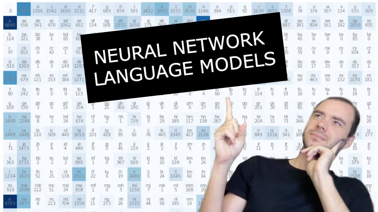
00:19:14.400 | And then here's the code that I came up with to try to make this a little bit nicer.

00:19:19.320 | We create a figure, we plot n, and then we visualize a bunch of things later.

00:19:27.480 | Let me just run it so you get a sense of what this is.

00:19:32.240 | So you see here that we have the array spaced out, and every one of these is basically b

00:19:40.040 | follows g zero times, b follows h 41 times, so a follows j 175 times.

00:19:48.160 | And so what you can see that I'm doing here is first I show that entire array, and then

00:19:53.240 | I iterate over all the individual little cells here, and I create a character string here,

00:19:59.440 | which is the inverse mapping i to s of the integer i and the integer j.

00:20:04.680 | So those are the bigrams in a character representation.

00:20:08.800 | And then I plot just the bigram text, and then I plot the number of times that this

00:20:14.400 | bigram occurs.

00:20:16.240 | Now the reason that there's a dot item here is because when you index into these arrays,

00:20:21.120 | these are torch tensors, you see that we still get a tensor back.

00:20:26.160 | So the type of this thing, you'd think it would be just an integer, 149, but it's actually

00:20:30.140 | a torch dot tensor.

00:20:32.160 | And so if you do dot item, then it will pop out that individual integer.

00:20:38.640 | So it'll just be 149.

00:20:40.840 | So that's what's happening there.

00:20:42.600 | And these are just some options to make it look nice.

00:20:45.440 | So what is the structure of this array?

00:20:46.840 | We have all these counts, and we see that some of them occur often, and some of them

00:20:52.280 | do not occur often.

00:20:54.120 | Now if you scrutinize this carefully, you will notice that we're not actually being

00:20:57.320 | very clever.

00:20:58.840 | That's because when you come over here, you'll notice that, for example, we have an entire

00:21:02.760 | row of completely zeros.

00:21:04.800 | And that's because the end character is never possibly going to be the first character of

00:21:09.080 | a bigram, because we're always placing these end tokens at the end of the bigram.

00:21:14.360 | Similarly, we have entire columns of zeros here, because the s character will never possibly

00:21:21.040 | be the second element of a bigram, because we always start with s and we end with e,

00:21:25.880 | and we only have the words in between.

00:21:27.840 | So we have an entire column of zeros, an entire row of zeros.

00:21:31.960 | And in this little two by two matrix here as well, the only one that can possibly happen

00:21:36.000 | is if s directly follows e.

00:21:38.580 | That can be non-zero if we have a word that has no letters.

00:21:43.240 | So in that case, there's no letters in the word.

00:21:44.760 | It's an empty word, and we just have s follows e.

00:21:47.520 | But the other ones are just not possible.

00:21:50.320 | And so we're basically wasting space.

00:21:51.820 | And not only that, but the s and the e are getting very crowded here.

00:21:55.600 | I was using these brackets because there's convention in natural language processing

00:21:59.440 | to use these kinds of brackets to denote special tokens, but we're going to use something else.

00:22:05.360 | So let's fix all this and make it prettier.

00:22:08.380 | We're not actually going to have two special tokens.

00:22:10.440 | We're only going to have one special token.

00:22:13.140 | So we're going to have n by n array of 27 by set 27 instead.

00:22:19.160 | Instead of having two, we will just have one, and I will call it a dot.

00:22:27.520 | Let me swing this over here.

00:22:30.600 | Now one more thing that I would like to do is I would actually like to make this special

00:22:34.360 | character have position zero.

00:22:36.480 | And I would like to offset all the other letters off.

00:22:39.000 | I find that a little bit more pleasing.

00:22:42.800 | So we need a plus one here so that the first character, which is a, will start at one.

00:22:50.040 | So s to i will now be a starts at one and dot is zero.

00:22:56.120 | And i to s, of course, we're not changing this because i to s just creates a reverse

00:23:00.420 | mapping and this will work fine.

00:23:02.400 | So one is a, two is b, zero is dot.

00:23:06.760 | So we've reversed that.

00:23:08.160 | Here we have a dot and a dot.

00:23:13.160 | This should work fine.

00:23:14.960 | Make sure I start at zeros.

00:23:17.840 | Count.

00:23:18.920 | And then here we don't go up to 28, we go up to 27.

00:23:22.840 | And this should just work.

00:23:26.960 | Okay.

00:23:31.960 | So we see that dot dot never happened.

00:23:33.640 | It's at zero because we don't have empty words.

00:23:36.680 | And this row here now is just very simply the counts for all the first letters.

00:23:43.680 | So j starts a word, h starts a word, i starts a word, et cetera.

00:23:49.720 | And then these are all the ending characters.

00:23:53.200 | And in between we have the structure of what characters follow each other.

00:23:57.200 | So this is the counts array of our entire dataset.

00:24:01.840 | So this array actually has all the information necessary for us to actually sample from this

00:24:06.340 | bigram character level language model.

00:24:09.960 | And roughly speaking, what we're going to do is we're just going to start following

00:24:13.640 | these probabilities and these counts, and we're going to start sampling from the model.

00:24:19.000 | So in the beginning, of course, we start with the dot, the start token dot.

00:24:24.760 | So to sample the first character of a name, we're looking at this row here.

00:24:30.720 | So we see that we have the counts and those counts externally are telling us how often

00:24:35.720 | any one of these characters is to start a word.

00:24:39.740 | So if we take this n and we grab the first row, we can do that by using just indexing

00:24:47.340 | as zero and then using this notation, colon, for the rest of that row.

00:24:53.860 | So n zero colon is indexing into the zeroth row and then it's grabbing all the columns.

00:25:02.140 | And so this will give us a one dimensional array of the first row.

00:25:06.320 | So 0 4 4 10, you know, 0 4 4 10, 1 3 0 6, 1 5 4 2, etc.

00:25:13.020 | It's just the first row.

00:25:14.560 | The shape of this is 27.

00:25:17.420 | Just the row of 27.

00:25:20.180 | And the other way that you can do this also is you just you don't actually give this,

00:25:23.920 | you just grab the zeroth row like this.

00:25:26.420 | This is equivalent.

00:25:28.300 | Now these are the counts and now what we'd like to do is we'd like to basically sample

00:25:33.700 | from this.

00:25:34.700 | Since these are the raw counts, we actually have to convert this to probabilities.

00:25:39.300 | So we create a probability vector.

00:25:43.100 | So we'll take n of zero and we'll actually convert this to float first.

00:25:48.860 | OK, so these integers are converted to float, floating point numbers.

00:25:54.300 | And the reason we're creating floats is because we're about to normalize these counts.

00:25:59.060 | So to create a probability distribution here, we want to divide.

00:26:04.020 | We basically want to do p, p, p divide p dot sum.

00:26:09.860 | And now we get a vector of smaller numbers.

00:26:12.280 | And these are now probabilities.

00:26:13.900 | So of course, because we divided by the sum, the sum of p now is one.

00:26:18.980 | So this is a nice proper probability distribution.

00:26:21.220 | It sums to one.

00:26:22.220 | And this is giving us the probability for any single character to be the first character

00:26:26.420 | of a word.

00:26:28.140 | So now we can try to sample from this distribution.

00:26:30.900 | To sample from these distributions, we're going to use tors dot multinomial, which I've

00:26:34.580 | pulled up here.

00:26:36.400 | So tors dot multinomial returns samples from the multinomial probability distribution,

00:26:43.460 | which is a complicated way of saying you give me probabilities and I will give you integers,

00:26:48.220 | which are sampled according to the probability distribution.

00:26:51.820 | So this is the signature of the method.

00:26:53.420 | And to make everything deterministic, we're going to use a generator object in PyTorch.

00:26:59.460 | So this makes everything deterministic.

00:27:01.160 | So when you run this on your computer, you're going to get the exact same results that I'm

00:27:04.940 | getting here on my computer.

00:27:07.440 | So let me show you how this works.

00:27:12.980 | Here's the deterministic way of creating a torch generator object, seeding it with some

00:27:19.180 | number that we can agree on, so that seeds a generator, gives us an object g.

00:27:24.940 | And then we can pass that g to a function that creates here random numbers, tors dot

00:27:32.180 | rand creates random numbers, three of them.

00:27:34.940 | And it's using this generator object as a source of randomness.

00:27:40.580 | So without normalizing it, I can just print.

00:27:46.700 | This is sort of like numbers between zero and one that are random according to this

00:27:50.500 | thing.

00:27:51.500 | And whenever I run it again, I'm always going to get the same result because I keep using

00:27:55.500 | the same generator object, which I'm seeding here.

00:27:59.000 | And then if I divide to normalize, I'm going to get a nice probability distribution of

00:28:05.380 | just three elements.

00:28:07.780 | And then we can use tors dot multinomial to draw samples from it.

00:28:11.360 | So this is what that looks like.

00:28:13.900 | Tors dot multinomial will take the torch tensor of probability distributions.

00:28:21.220 | Then we can ask for a number of samples, let's say 20.

00:28:25.140 | Replacement equals true means that when we draw an element, we can draw it and then we

00:28:30.980 | can put it back into the list of eligible indices to draw again.

00:28:36.100 | And we have to specify replacement as true because by default, for some reason, it's

00:28:41.260 | false.

00:28:42.260 | You know, it's just something to be careful with.

00:28:45.980 | And the generator is passed in here.

00:28:47.580 | So we're going to always get deterministic results, the same results.

00:28:51.480 | So if I run these two, we're going to get a bunch of samples from this distribution.

00:28:57.260 | Now you'll notice here that the probability for the first element in this tensor is 60%.

00:29:04.700 | So in these 20 samples, we'd expect 60% of them to be zero.

00:29:10.900 | We'd expect 30% of them to be one.

00:29:14.500 | And because the element index two has only 10% probability, very few of these samples

00:29:20.820 | should be two.

00:29:22.380 | And indeed, we only have a small number of twos.

00:29:25.660 | We can sample as many as we like.

00:29:29.220 | And the more we sample, the more these numbers should roughly have the distribution here.

00:29:36.080 | So we should have lots of zeros, half as many ones, and we should have three times as few

00:29:45.340 | ones, and three times as few twos.

00:29:51.940 | So you see that we have very few twos, we have some ones, and most of them are zero.

00:29:55.940 | So that's what torsion multinomial is doing.

00:29:59.060 | For us here, we are interested in this row, we've created this p here, and now we can

00:30:07.440 | sample from it.

00:30:09.840 | So if we use the same seed, and then we sample from this distribution, let's just get one

00:30:15.800 | sample, then we see that the sample is, say, 13.

00:30:22.900 | So this will be the index.

00:30:26.080 | You see how it's a tensor that wraps 13?

00:30:28.940 | We again have to use .item to pop out that integer.

00:30:33.160 | And now index would be just the number 13.

00:30:37.640 | And of course, we can map the I2S of IX to figure out exactly which character we're sampling

00:30:45.720 | here.

00:30:46.720 | We're sampling M. So we're saying that the first character is M in our generation.

00:30:53.380 | And just looking at the row here, M was drawn, and we can see that M actually starts a large

00:30:58.560 | number of words.

00:31:00.320 | M started 2,500 words out of 32,000 words.

00:31:04.880 | So almost a bit less than 10% of the words start with M. So this is actually a fairly

00:31:10.120 | likely character to draw.

00:31:15.440 | So that would be the first character of our word.

00:31:17.240 | And now we can continue to sample more characters, because now we know that M is already sampled.

00:31:24.940 | So now to draw the next character, we will come back here, and we will look for the row

00:31:30.920 | that starts with M. So you see M, and we have a row here.

00:31:36.900 | So we see that M. is 516, MA is this many, MB is this many, etc.

00:31:43.920 | So these are the counts for the next row, and that's the next character that we are

00:31:46.840 | going to now generate.

00:31:48.840 | So I think we are ready to actually just write out the loop, because I think you're starting

00:31:52.120 | to get a sense of how this is going to go.

00:31:54.720 | We always begin at index 0, because that's the start token.

00:32:02.560 | And then while true, we're going to grab the row corresponding to index that we're currently

00:32:09.440 | on.

00:32:10.440 | So that's N array at ix, converted to float is our P.

00:32:19.400 | Then we normalize this P to sum to 1.

00:32:24.040 | I accidentally ran the infinite loop.

00:32:28.360 | We normalize P to sum to 1.

00:32:30.960 | Then we need this generator object.

00:32:32.960 | We're going to initialize up here, and we're going to draw a single sample from this distribution.

00:32:41.040 | And then this is going to tell us what index is going to be next.

00:32:46.760 | If the index sampled is 0, then that's now the end token.

00:32:52.840 | So we will break.

00:32:54.640 | Otherwise, we are going to print s2i of ix.

00:33:02.400 | i2s of ix.

00:33:05.680 | And that's pretty much it.

00:33:07.440 | We're just — this should work.

00:33:10.360 | Okay, more.

00:33:12.280 | So that's the name that we've sampled.

00:33:14.880 | We started with M, the next step was O, then R, and then dot.

00:33:21.680 | And this dot, we printed here as well.

00:33:25.040 | So let's now do this a few times.

00:33:30.200 | So let's actually create an out list here.

00:33:37.360 | And instead of printing, we're going to append.

00:33:39.920 | So out.append this character.

00:33:44.640 | And then here, let's just print it at the end.

00:33:47.080 | So let's just join up all the outs, and we're just going to print more.

00:33:51.040 | Now, we're always getting the same result because of the generator.

00:33:55.360 | So if we want to do this a few times, we can go for i in range 10.

00:34:00.840 | We can sample 10 names, and we can just do that 10 times.

00:34:05.960 | And these are the names that we're getting out.

00:34:08.800 | Let's do 20.

00:34:14.480 | I'll be honest with you, this doesn't look right.

00:34:16.720 | So I started a few minutes to convince myself that it actually is right.

00:34:20.680 | The reason these samples are so terrible is that bigram language model is actually just

00:34:26.280 | really terrible.

00:34:27.280 | We can generate a few more here.

00:34:29.560 | And you can see that they're kind of like — they're name-like a little bit, like

00:34:33.200 | Ianu, O'Reilly, et cetera, but they're just totally messed up.

00:34:38.920 | And I mean, the reason that this is so bad — like, we're generating H as a name,

00:34:43.240 | but you have to think through it from the model's eyes.

00:34:46.680 | It doesn't know that this H is the very first H.

00:34:49.520 | All it knows is that H was previously, and now how likely is H the last character?

00:34:55.040 | Well, it's somewhat likely, and so it just makes it last character.

00:34:59.240 | It doesn't know that there were other things before it or there were not other things before

00:35:03.200 | it.

00:35:04.200 | And so that's why it's generating all these, like, nonsense names.

00:35:08.480 | Another way to do this is to convince yourself that this is actually doing something reasonable,

00:35:14.600 | even though it's so terrible, is these little p's here are 27, right?

00:35:21.200 | Like 27.

00:35:23.380 | So how about if we did something like this?

00:35:26.600 | Instead of p having any structure whatsoever, how about if p was just torch.once(27).

00:35:37.440 | By default, this is a float 32, so this is fine.

00:35:40.480 | Divide 27.

00:35:43.120 | So what I'm doing here is this is the uniform distribution, which will make everything equally

00:35:48.160 | likely.

00:35:50.120 | And we can sample from that.

00:35:52.100 | So let's see if that does any better.

00:35:55.080 | So this is what you have from a model that is completely untrained, where everything

00:35:59.200 | is equally likely.

00:36:00.820 | So it's obviously garbage.

00:36:02.560 | And then if we have a trained model, which is trained on just bigrams, this is what we

00:36:07.680 | get.

00:36:08.680 | So you can see that it is more name-like.

00:36:10.600 | It is actually working.

00:36:12.000 | It's just bigram is so terrible, and we have to do better.

00:36:16.720 | Now next, I would like to fix an inefficiency that we have going on here, because what we're

00:36:20.760 | doing here is we're always fetching a row of n from the counts matrix up ahead.

00:36:26.720 | And then we're always doing the same things.

00:36:28.080 | We're converting to float and we're dividing.

00:36:30.080 | And we're doing this every single iteration of this loop.

00:36:32.960 | And we just keep renormalizing these rows over and over again.

00:36:35.080 | And it's extremely inefficient and wasteful.

00:36:37.580 | So what I'd like to do is I'd like to actually prepare a matrix, capital P, that will just

00:36:42.120 | have the probabilities in it.

00:36:44.160 | So in other words, it's going to be the same as the capital N matrix here of counts.

00:36:48.180 | But every single row will have the row of probabilities that is normalized to 1, indicating

00:36:53.440 | the probability distribution for the next character given the character before it, as

00:36:58.760 | defined by which row we're in.

00:37:01.760 | So basically what we'd like to do is we'd like to just do it up front here.

00:37:05.280 | And then we would like to just use that row here.

00:37:08.360 | So here, we would like to just do P equals P of IX instead.

00:37:15.120 | The other reason I want to do this is not just for efficiency, but also I would like

00:37:18.120 | us to practice these n-dimensional tensors.

00:37:21.360 | And I'd like us to practice their manipulation, and especially something that's called broadcasting,

00:37:25.120 | that we'll go into in a second.

00:37:27.160 | We're actually going to have to become very good at these tensor manipulations, because

00:37:31.000 | if we're going to build out all the way to transformers, we're going to be doing some

00:37:34.040 | pretty complicated array operations for efficiency.

00:37:37.600 | And we need to really understand that and be very good at it.

00:37:42.460 | So intuitively, what we want to do is we first want to grab the floating point copy of N.

00:37:48.440 | And I'm mimicking the line here, basically.

00:37:51.160 | And then we want to divide all the rows so that they sum to 1.

00:37:55.880 | So we'd like to do something like this, P divide P dot sum.

00:38:00.840 | But now we have to be careful, because P dot sum actually produces a sum--sorry, P equals

00:38:09.120 | N dot float copy.

00:38:10.920 | P dot sum produces a--sums up all of the counts of this entire matrix N and gives us a single

00:38:19.060 | number of just the summation of everything.

00:38:21.460 | So that's not the way we want to divide.

00:38:23.600 | We want to simultaneously and in parallel divide all the rows by their respective sums.

00:38:30.800 | So what we have to do now is we have to go into documentation for torch dot sum.

00:38:36.100 | And we can scroll down here to a definition that is relevant to us, which is where we

00:38:40.120 | don't only provide an input array that we want to sum, but we also provide the dimension

00:38:45.240 | along which we want to sum.

00:38:46.720 | And in particular, we want to sum up over rows.

00:38:52.560 | Now one more argument that I want you to pay attention to here is the keep_dim is false.

00:38:58.080 | If keep_dim is true, then the output tensor is of the same size as input, except of course

00:39:03.100 | the dimension along which you summed, which will become just 1.

00:39:07.600 | But if you pass in keep_dim as false, then this dimension is squeezed out.

00:39:14.580 | And so torch dot sum not only does the sum and collapses dimension to be of size 1, but

00:39:19.120 | in addition, it does what's called a squeeze, where it squeezes out that dimension.

00:39:24.780 | So basically what we want here is we instead want to do p dot sum of some axis.

00:39:31.040 | And in particular, notice that p dot shape is 27 by 27.

00:39:35.820 | So when we sum up across axis 0, then we would be taking the 0th dimension and we would be

00:39:40.580 | summing across it.

00:39:42.860 | So when keep_dim is true, then this thing will not only give us the counts along the

00:39:50.500 | columns, but notice that basically the shape of this is 1 by 27.

00:39:55.640 | We just get a row vector.

00:39:57.700 | And the reason we get a row vector here, again, is because we pass in 0th dimension.

00:40:01.080 | So this 0th dimension becomes 1.

00:40:03.180 | And we've done a sum, and we get a row.

00:40:06.060 | And so basically we've done the sum this way, vertically, and arrived at just a single 1

00:40:11.500 | by 27 vector of counts.

00:40:15.540 | What happens when you take out keep_dim is that we just get 27.

00:40:19.740 | So it squeezes out that dimension, and we just get a one-dimensional vector of size

00:40:25.340 | 27.

00:40:28.780 | Now we don't actually want 1 by 27 row vector, because that gives us the counts, or the sums,

00:40:35.940 | across the columns.

00:40:39.660 | We actually want to sum the other way, along dimension 1.

00:40:42.940 | And you'll see that the shape of this is 27 by 1.

00:40:45.900 | So it's a column vector.

00:40:47.620 | It's a 27 by 1 vector of counts.

00:40:54.100 | And that's because what's happened here is that we're going horizontally, and this 27

00:40:57.820 | by 27 matrix becomes a 27 by 1 array.

00:41:03.740 | And you'll notice, by the way, that the actual numbers of these counts are identical.

00:41:10.820 | And that's because this special array of counts here comes from bigram statistics.

00:41:15.020 | And actually, it just so happens by chance, or because of the way this array is constructed,

00:41:20.340 | that the sums along the columns, or along the rows, horizontally or vertically, is identical.

00:41:26.380 | But actually what we want to do in this case is we want to sum across the rows, horizontally.

00:41:32.420 | So what we want here is p.sum of 1 with keep_dim true, 27 by 1 column vector.

00:41:39.740 | And now what we want to do is we want to divide by that.

00:41:44.900 | Now we have to be careful here again.

00:41:46.400 | Is it possible to take what's a p.shape you see here, 27 by 27, is it possible to take

00:41:53.500 | a 27 by 27 array and divide it by what is a 27 by 1 array?

00:42:01.500 | Is that an operation that you can do?

00:42:04.140 | And whether or not you can perform this operation is determined by what's called broadcasting

00:42:07.420 | rules.

00:42:08.480 | So if you just search broadcasting semantics in Torch, you'll notice that there's a special

00:42:13.100 | definition for what's called broadcasting, that for whether or not these two arrays can

00:42:20.380 | be combined in a binary operation like division.

00:42:24.120 | So the first condition is each tensor has at least one dimension, which is the case

00:42:27.500 | for us.

00:42:28.780 | And then when iterating over the dimension sizes, starting at the trailing dimension,

00:42:32.580 | the dimension sizes must either be equal, one of them is one, or one of them does not

00:42:36.420 | exist.

00:42:39.100 | So let's do that.

00:42:40.460 | We need to align the two arrays and their shapes, which is very easy because both of

00:42:45.340 | these shapes have two elements, so they're aligned.

00:42:48.300 | Then we iterate over from the right and going to the left.

00:42:52.560 | Each dimension must be either equal, one of them is a one, or one of them does not exist.

00:42:58.140 | So in this case, they're not equal, but one of them is a one.

00:43:00.620 | So this is fine.

00:43:02.120 | And then this dimension, they're both equal.

00:43:04.220 | So this is fine.

00:43:06.100 | So all the dimensions are fine, and therefore this operation is broadcastable.

00:43:12.100 | So that means that this operation is allowed.

00:43:14.740 | And what is it that these arrays do when you divide 27 by 27 by 27 by one?

00:43:20.040 | What it does is that it takes this dimension one, and it stretches it out, it copies it

00:43:26.100 | to match 27 here in this case.

00:43:29.220 | So in our case, it takes this column vector, which is 27 by one, and it copies it 27 times

00:43:36.800 | to make these both be 27 by 27 internally.

00:43:40.680 | You can think of it that way.

00:43:41.680 | And so it copies those counts, and then it does an element-wise division, which is what

00:43:47.900 | we want because these counts, we want to divide by them on every single one of these columns

00:43:53.060 | in this matrix.

00:43:55.000 | So this actually, we expect, will normalize every single row.

00:43:59.960 | And we can check that this is true by taking the first row, for example, and taking its

00:44:04.860 | sum.

00:44:05.860 | We expect this to be one because it's now normalized.

00:44:10.580 | And then we expect this now because if we actually correctly normalize all the rows,

00:44:15.740 | we expect to get the exact same result here.

00:44:17.900 | So let's run this.

00:44:18.900 | It's the exact same result.

00:44:21.560 | So this is correct.

00:44:23.160 | So now I would like to scare you a little bit.

00:44:25.620 | You actually have to like, I basically encourage you very strongly to read through broadcasting

00:44:29.320 | semantics and I encourage you to treat this with respect.

00:44:32.960 | And it's not something to play fast and loose with.

00:44:35.340 | It's something to really respect, really understand, and look up maybe some tutorials for broadcasting

00:44:39.580 | and practice it and be careful with it because you can very quickly run into bugs.

00:44:44.020 | Let me show you what I mean.

00:44:47.380 | You see how here we have p.sum of one, keep them as true.

00:44:50.680 | The shape of this is 27 by one.

00:44:53.200 | Let me take out this line just so we have the n and then we can see the counts.

00:44:58.640 | We can see that this is all the counts across all the rows and it's 27 by one column vector,

00:45:06.280 | right?

00:45:07.280 | Now suppose that I tried to do the following, but I erase keep them as true here.

00:45:14.160 | What does that do?

00:45:15.160 | If keep them is not true, it's false.

00:45:17.360 | And remember, according to documentation, it gets rid of this dimension one, it squeezes

00:45:21.920 | it out.

00:45:23.080 | So basically we just get all the same counts, the same result, except the shape of it is

00:45:27.520 | not 27 by one, it's just 27, the one that disappears.

00:45:31.900 | But all the counts are the same.

00:45:34.340 | So you'd think that this divide that would work.

00:45:40.280 | First of all, can we even write this and is it even expected to run?

00:45:45.160 | Is it broadcastable?

00:45:46.160 | Let's determine if this result is broadcastable.

00:45:49.320 | P dot sum at one is shape is 27.

00:45:53.120 | This is 27 by 27.

00:45:54.600 | So 27 by 27 broadcasting into 27.

00:46:00.460 | So now rules of broadcasting number one, align all the dimensions on the right, done.

00:46:06.440 | Now iteration over all the dimensions starting from the right, going to the left.

00:46:10.360 | All the dimensions must either be equal.

00:46:13.200 | One of them must be one or one of them does not exist.

00:46:16.120 | So here they are all equal.

00:46:17.960 | Here the dimension does not exist.

00:46:20.160 | So internally what broadcasting will do is it will create a one here.

00:46:24.560 | And then we see that one of them is a one and this will get copied and this will run,

00:46:30.400 | this will broadcast.

00:46:31.960 | Okay, so you'd expect this to work because we are, this broadcasts and this, we can divide

00:46:42.880 | this.

00:46:43.880 | Now if I run this, you'd expect it to work, but it doesn't.

00:46:48.280 | You actually get garbage.

00:46:49.280 | You get a wrong result because this is actually a bug.

00:46:52.640 | This keep dim equals true makes it work.

00:47:00.840 | This is a bug.

00:47:03.040 | In both cases, we are doing the correct counts.

00:47:06.440 | We are summing up across the rows, but keep dim is saving us and making it work.

00:47:11.720 | So in this case, I'd like to encourage you to potentially like pause this video at this

00:47:15.320 | point and try to think about why this is buggy and why the keep dim was necessary here.

00:47:21.320 | Okay, so the reason to do for this is I'm trying to hint it here when I was sort of

00:47:27.360 | giving you a bit of a hint on how this works.

00:47:29.720 | This 27 vector internally inside the broadcasting, this becomes a one by 27 and one by 27 is

00:47:37.640 | a row vector, right?

00:47:39.840 | And now we are dividing 27 by 27 by one by 27 and torch will replicate this dimension.

00:47:46.100 | So basically it will take, it will take this row vector and it will copy it vertically

00:47:54.160 | now 27 times.

00:47:56.380 | So the 27 by 27 lines exactly and element wise divides.

00:48:00.520 | And so basically what's happening here is we're actually normalizing the columns instead

00:48:06.420 | of normalizing the rows.

00:48:09.640 | So you can check that what's happening here is that P at zero, which is the first row

00:48:14.120 | of P dot sum is not one, it's seven.

00:48:18.800 | It is the first column as an example that sums to one.

00:48:23.840 | So to summarize, where does the issue come from?

00:48:26.640 | The issue comes from the silent adding of a dimension here, because in broadcasting

00:48:30.840 | rules, you align on the right and go from right to left.

00:48:33.960 | And if dimension doesn't exist, you create it.

00:48:36.420 | So that's where the problem happens.

00:48:38.080 | We still did the counts correctly.

00:48:39.520 | We did the counts across the rows and we got the counts on the right here as a column vector.

00:48:45.800 | But because the keyptons was true, this dimension was discarded and now we just have a vector

00:48:50.360 | of 27.

00:48:51.680 | And because of broadcasting the way it works, this vector of 27 suddenly becomes a row vector.

00:48:57.240 | And then this row vector gets replicated vertically.

00:49:00.120 | And that every single point we are dividing by the count in the opposite direction.

00:49:07.520 | So this thing just doesn't work.

00:49:11.640 | This needs to be keyptons equals true in this case.

00:49:14.380 | So then we have that P at zero is normalized.

00:49:20.120 | And conversely, the first column you'd expect to potentially not be normalized.

00:49:24.840 | And this is what makes it work.

00:49:27.840 | So pretty subtle.

00:49:29.600 | And hopefully this helps to scare you, that you should have respect for broadcasting,

00:49:34.400 | be careful, check your work, and understand how it works under the hood and make sure

00:49:39.200 | that it's broadcasting in the direction that you like.

00:49:41.160 | Otherwise, you're going to introduce very subtle bugs, very hard to find bugs.

00:49:45.360 | And just be careful.

00:49:46.840 | One more note on efficiency.

00:49:48.440 | We don't want to be doing this here because this creates a completely new tensor that

00:49:53.040 | we store into P. We prefer to use in-place operations if possible.

00:49:58.040 | So this would be an in-place operation, has the potential to be faster.

00:50:01.960 | It doesn't create new memory under the hood.

00:50:04.680 | And then let's erase this.

00:50:06.420 | We don't need it.

00:50:08.280 | And let's also just do fewer, just so I'm not wasting space.

00:50:14.280 | Okay, so we're actually in a pretty good spot now.

00:50:17.160 | We trained a bigram language model, and we trained it really just by counting how frequently

00:50:22.900 | any pairing occurs and then normalizing so that we get a nice property distribution.

00:50:28.120 | So really these elements of this array P are really the parameters of our bigram language

00:50:33.080 | model, giving us and summarizing the statistics of these bigrams.

00:50:37.140 | So we trained the model, and then we know how to sample from the model.

00:50:40.320 | We just iteratively sample the next character and feed it in each time and get the next

00:50:45.680 | character.

00:50:46.680 | Now, what I'd like to do is I'd like to somehow evaluate the quality of this model.

00:50:51.320 | We'd like to somehow summarize the quality of this model into a single number.

00:50:55.400 | How good is it at predicting the training set?

00:50:59.280 | And as an example, so in the training set, we can evaluate now the training loss.

00:51:04.480 | And this training loss is telling us about sort of the quality of this model in a single

00:51:08.520 | number, just like we saw in micrograd.

00:51:12.120 | So let's try to think through the quality of the model and how we would evaluate it.

00:51:16.160 | Basically, what we're going to do is we're going to copy paste this code that we previously

00:51:21.440 | used for counting.

00:51:24.440 | And let me just print the bigrams first.

00:51:26.160 | We're going to use f strings, and I'm going to print character one followed by character

00:51:30.480 | two.

00:51:31.480 | These are the bigrams.

00:51:32.480 | And then I don't want to do it for all the words, just do the first three words.

00:51:36.240 | So here we have Emma, Olivia, and Ava bigrams.

00:51:40.360 | Now what we'd like to do is we'd like to basically look at the probability that the model assigns

00:51:46.120 | to every one of these bigrams.

00:51:48.400 | So in other words, we can look at the probability, which is summarized in the matrix P of IX1,

00:51:54.160 | and then we can print it here as probability.

00:52:00.920 | And because these probabilities are way too large, let me percent or colon .4f to truncate

00:52:07.560 | it a bit.

00:52:09.400 | So what do we have here?

00:52:10.400 | We're looking at the probabilities that the model assigns to every one of these bigrams

00:52:13.840 | in the dataset.

00:52:15.440 | And so we can see some of them are 4%, 3%, et cetera.

00:52:18.880 | Just to have a measuring stick in our mind, by the way, we have 27 possible characters

00:52:23.880 | or tokens.

00:52:24.960 | And if everything was equally likely, then you'd expect all these probabilities to be

00:52:29.160 | 4% roughly.

00:52:32.640 | So anything above 4% means that we've learned something useful from these bigram statistics.

00:52:37.240 | And you see that roughly some of these are 4%, but some of them are as high as 40%, 35%,

00:52:43.360 | and so on.

00:52:44.360 | So you see that the model actually assigned a pretty high probability to whatever's in

00:52:47.440 | the training set.

00:52:48.480 | And so that's a good thing.

00:52:50.960 | Especially if you have a very good model, you'd expect that these probabilities should

00:52:53.840 | be near 1, because that means that your model is correctly predicting what's going to come

00:52:58.120 | next, especially on the training set where you trained your model.

00:53:03.000 | So now we'd like to think about how can we summarize these probabilities into a single

00:53:07.900 | number that measures the quality of this model?

00:53:11.920 | Now when you look at the literature into maximum likelihood estimation and statistical modeling

00:53:16.160 | and so on, you'll see that what's typically used here is something called the likelihood.

00:53:21.720 | And the likelihood is the product of all of these probabilities.

00:53:26.120 | And so the product of all of these probabilities is the likelihood.

00:53:29.460 | And it's really telling us about the probability of the entire data set assigned by the model

00:53:36.640 | that we've trained.

00:53:37.880 | And that is a measure of quality.

00:53:39.620 | So the product of these should be as high as possible when you are training the model

00:53:44.560 | and when you have a good model.

00:53:46.520 | Your product of these probabilities should be very high.

00:53:50.560 | Now because the product of these probabilities is an unwieldy thing to work with, you can

00:53:54.560 | see that all of them are between 0 and 1.

00:53:56.480 | So your product of these probabilities will be a very tiny number.

00:54:01.100 | So for convenience, what people work with usually is not the likelihood, but they work

00:54:05.240 | with what's called the log likelihood.

00:54:08.080 | So the product of these is the likelihood.

00:54:11.040 | To get the log likelihood, we just have to take the log of the probability.

00:54:15.240 | And so the log of the probability here, I have the log of x from 0 to 1.

00:54:19.900 | The log is a, you see here, monotonic transformation of the probability, where if you pass in 1,

00:54:27.400 | you get 0.

00:54:29.020 | So probability 1 gets you log probability of 0.

00:54:32.440 | And then as you go lower and lower probability, the log will grow more and more negative until

00:54:37.040 | all the way to negative infinity at 0.

00:54:42.080 | So here we have a log prob, which is really just a torsion log of probability.

00:54:47.080 | Let's print it out to get a sense of what that looks like.

00:54:50.240 | Log prob also 0.4f.

00:54:56.800 | So as you can see, when we plug in numbers that are very close, some of our higher numbers,

00:55:01.520 | we get closer and closer to 0.

00:55:03.660 | And then if we plug in very bad probabilities, we get more and more negative number.

00:55:08.120 | That's bad.

00:55:09.760 | So and the reason we work with this is for large extent convenience, right?

00:55:15.560 | Because we have mathematically that if you have some product, a times b times c, of all

00:55:19.360 | these probabilities, right?

00:55:21.360 | The likelihood is the product of all these probabilities.

00:55:25.620 | And the log of these is just log of a plus log of b plus log of c.

00:55:35.260 | If you remember your logs from your high school or undergrad and so on.

00:55:39.960 | So we have that basically, the likelihood is the product of probabilities.

00:55:43.420 | The log likelihood is just the sum of the logs of the individual probabilities.

00:55:48.980 | So log likelihood starts at 0.

00:55:54.860 | And then log likelihood here, we can just accumulate simply.

00:56:00.580 | And then the end, we can print this.

00:56:05.660 | Print the log likelihood.

00:56:07.660 | F strings.

00:56:10.180 | Maybe you're familiar with this.

00:56:14.100 | So log likelihood is negative 38.

00:56:18.540 | Okay.

00:56:21.420 | Now we actually want -- so how high can log likelihood get?

00:56:27.900 | It can go to 0.

00:56:30.020 | So when all the probabilities are 1, log likelihood will be 0.

00:56:33.020 | And then when all the probabilities are lower, this will grow more and more negative.

00:56:37.580 | Now we don't actually like this because what we'd like is a loss function.

00:56:41.340 | And a loss function has the semantics that low is good.

00:56:46.500 | Because we're trying to minimize the loss.

00:56:48.340 | So we actually need to invert this.

00:56:50.540 | And that's what gives us something called the negative log likelihood.

00:56:56.300 | Negative log likelihood is just negative of the log likelihood.

00:57:04.060 | These are F strings, by the way, if you'd like to look this up.

00:57:06.780 | Negative log likelihood equals.

00:57:09.540 | So negative log likelihood now is just negative of it.

00:57:12.240 | And so the negative log likelihood is a very nice loss function.

00:57:16.140 | Because the lowest it can get is 0.

00:57:19.980 | And the higher it is, the worse off the predictions are that you're making.

00:57:24.900 | And then one more modification to this that sometimes people do is that for convenience,

00:57:29.300 | they actually like to normalize by -- they like to make it an average instead of a sum.

00:57:34.620 | And so here, let's just keep some counts as well.

00:57:39.480 | So n plus equals 1 starts at 0.

00:57:43.020 | And then here, we can have sort of like a normalized log likelihood.

00:57:50.660 | If we just normalize it by the count, then we will sort of get the average log likelihood.

00:57:55.940 | So this would be usually our loss function here.

00:57:59.980 | This is what we would use.

00:58:02.480 | So our loss function for the training set assigned by the model is 2.4.

00:58:06.620 | That's the quality of this model.

00:58:08.740 | And the lower it is, the better off we are.

00:58:10.700 | And the higher it is, the worse off we are.

00:58:13.740 | And the job of our training is to find the parameters that minimize the negative log

00:58:20.140 | likelihood loss.

00:58:23.140 | And that would be like a high-quality model.

00:58:25.140 | Okay, so to summarize, I actually wrote it out here.

00:58:28.240 | So our goal is to maximize likelihood, which is the product of all the probabilities assigned

00:58:34.420 | by the model.

00:58:35.420 | And we want to maximize this likelihood with respect to the model parameters.

00:58:39.420 | And in our case, the model parameters here are defined in the table.

00:58:43.660 | These numbers, the probabilities, are the model parameters sort of in our bigram language

00:58:48.580 | model so far.

00:58:49.580 | But you have to keep in mind that here we are storing everything in a table format,

00:58:53.820 | the probabilities.

00:58:54.820 | But what's coming up as a brief preview is that these numbers will not be kept explicitly,

00:59:00.340 | but these numbers will be calculated by a neural network.

00:59:03.340 | So that's coming up.

00:59:04.340 | And we want to change and tune the parameters of these neural networks.

00:59:08.260 | We want to change these parameters to maximize the likelihood, the product of the probabilities.

00:59:13.500 | Now maximizing the likelihood is equivalent to maximizing the log likelihood because log

00:59:17.900 | is a monotonic function.

00:59:20.180 | Here's the graph of log.

00:59:22.260 | And basically all it is doing is it's just scaling your, you can look at it as just a

00:59:27.520 | scaling of the loss function.

00:59:29.700 | And so the optimization problem here and here are actually equivalent because this is just

00:59:35.020 | scaling.

00:59:36.020 | You can look at it that way.

00:59:37.240 | And so these are two identical optimization problems.

00:59:42.460 | Maximizing the log likelihood is equivalent to minimizing the negative log likelihood.

00:59:46.420 | And then in practice, people actually minimize the average negative log likelihood to get

00:59:50.540 | numbers like 2.4.

00:59:53.180 | And then this summarizes the quality of your model.

00:59:56.460 | And we'd like to minimize it and make it as small as possible.

00:59:59.900 | And the lowest it can get is zero.

01:00:02.600 | And the lower it is, the better off your model is because it's assigning high probabilities

01:00:08.600 | to your data.

01:00:09.600 | Now let's estimate the probability over the entire training set just to make sure that

01:00:12.680 | we get something around 2.4.

01:00:15.160 | Let's run this over the entire, oops.

01:00:17.580 | Let's take out the print statement as well.

01:00:19.600 | Okay, 2.45 over the entire training set.

01:00:24.700 | Now what I'd like to show you is that you can actually evaluate the probability for

01:00:27.260 | any word that you want.

01:00:28.520 | So for example, if we just test a single word, Andre, and bring back the print statement,

01:00:36.040 | then you see that Andre is actually kind of like an unlikely word.

01:00:39.000 | Like on average, we take three log probability to represent it.

01:00:44.760 | And roughly that's because EJ apparently is very uncommon as an example.

01:00:50.200 | Now think through this.

01:00:52.440 | When I take Andre and I append Q and I test the probability of it, Andre Q, we actually

01:01:00.680 | get infinity.

01:01:03.240 | And that's because JQ has a 0% probability according to our model.

01:01:07.840 | So the log likelihood, so the log of zero will be negative infinity.

01:01:12.360 | We get infinite loss.

01:01:14.760 | So this is kind of undesirable, right?

01:01:15.980 | Because we plugged in a string that could be like a somewhat reasonable name.

01:01:19.400 | But basically what this is saying is that this model is exactly 0% likely to predict

01:01:24.600 | this name.

01:01:26.760 | And our loss is infinity on this example.

01:01:30.000 | And really what the reason for that is that J is followed by Q zero times.

01:01:36.560 | Where's Q?

01:01:37.960 | JQ is zero.

01:01:39.520 | And so JQ is 0% likely.

01:01:42.440 | So it's actually kind of gross and people don't like this too much.

01:01:45.420 | To fix this, there's a very simple fix that people like to do to sort of like smooth out

01:01:49.500 | your model a little bit.

01:01:50.500 | And it's called model smoothing.

01:01:52.340 | And roughly what's happening is that we will add some fake counts.

01:01:56.440 | So imagine adding a count of one to everything.

01:02:01.160 | So we add a count of one like this, and then we recalculate the probabilities.

01:02:07.980 | And that's model smoothing.

01:02:08.980 | And you can add as much as you like.

01:02:10.260 | You can add five and that will give you a smoother model.

01:02:13.140 | And the more you add here, the more uniform model you're going to have.

01:02:17.940 | And the less you add, the more peaked model you're going to have, of course.

01:02:22.500 | So one is like a pretty decent count to add.

01:02:25.940 | And that will ensure that there will be no zeros in our probability matrix P.

01:02:31.120 | And so this will of course change the generations a little bit.

01:02:33.800 | In this case, it didn't, but in principle it could.

01:02:36.780 | But what that's going to do now is that nothing will be infinity unlikely.

01:02:41.340 | So now our model will predict some other probability.

01:02:44.940 | And we see that JQ now has a very small probability.

01:02:47.860 | So the model still finds it very surprising that this was a word or a bigram, but we don't

01:02:52.020 | get negative infinity.

01:02:53.020 | So it's kind of like a nice fix that people like to apply sometimes, and it's called model

01:02:56.340 | smoothing.

01:02:57.340 | Okay, so we've now trained a respectable bigram character level language model.

01:03:01.660 | And we saw that we both sort of trained the model by looking at the counts of all the

01:03:06.780 | bigrams and normalizing the rows to get probability distributions.

01:03:11.660 | We saw that we can also then use those parameters of this model to perform sampling of new words.

01:03:19.700 | So we sample new names according to those distributions.

01:03:22.420 | And we also saw that we can evaluate the quality of this model.

01:03:25.640 | And the quality of this model is summarized in a single number, which is the negative

01:03:28.820 | log likelihood.

01:03:30.140 | And the lower this number is, the better the model is, because it is giving high probabilities

01:03:35.620 | to the actual next characters in all the bigrams in our training set.

01:03:40.340 | So that's all well and good, but we've arrived at this model explicitly by doing something

01:03:44.940 | that felt sensible.

01:03:46.260 | We were just performing counts, and then we were normalizing those counts.

01:03:51.180 | Now what I would like to do is I would like to take an alternative approach.

01:03:54.260 | We will end up in a very, very similar position, but the approach will look very different,

01:03:58.460 | because I would like to cast the problem of bigram character level language modeling into

01:04:02.460 | the neural network framework.

01:04:04.380 | And in the neural network framework, we're going to approach things slightly differently,

01:04:08.300 | but again, end up in a very similar spot.

01:04:10.300 | I'll go into that later.

01:04:12.100 | Now our neural network is going to be still a bigram character level language model.

01:04:17.420 | So it receives a single character as an input.

01:04:20.540 | Then there's neural network with some weights or some parameters w.

01:04:24.220 | And it's going to output the probability distribution over the next character in a sequence.

01:04:29.300 | And it's going to make guesses as to what is likely to follow this character that was

01:04:33.740 | input to the model.

01:04:36.140 | And then in addition to that, we're going to be able to evaluate any setting of the

01:04:39.900 | parameters of the neural net, because we have the loss function, the negative log likelihood.

01:04:45.160 | So we're going to take a look at this probability distributions, and we're going to use the

01:04:48.260 | labels, which are basically just the identity of the next character in that bigram, the

01:04:53.460 | second character.

01:04:54.880 | So knowing what second character actually comes next in the bigram allows us to then

01:04:59.140 | look at how high of a probability the model assigns to that character.

01:05:04.100 | And then we of course want the probability to be very high.

01:05:07.240 | And that is another way of saying that the loss is low.

01:05:10.960 | So we're going to use gradient based optimization then to tune the parameters of this network,

01:05:15.660 | because we have the loss function and we're going to minimize it.

01:05:18.600 | So we're going to tune the weights so that the neural net is correctly predicting the

01:05:22.220 | probabilities for the next character.

01:05:24.540 | So let's get started.

01:05:25.700 | The first thing I want to do is I want to compile the training set of this neural network.

01:05:29.660 | So create the training set of all the bigrams.

01:05:37.940 | And here I'm going to copy/paste this code, because this code iterates over all the bigrams.

01:05:47.580 | So here we start with the words, we iterate over all the bigrams, and previously, as you

01:05:51.380 | recall, we did the counts.

01:05:53.220 | But now we're not going to do counts.

01:05:54.640 | We're just creating a training set.

01:05:57.060 | Now this training set will be made up of two lists.

01:06:02.220 | We have the inputs and the targets, the labels.

01:06:09.720 | And these bigrams will denote x, y.

01:06:11.380 | Those are the characters, right?

01:06:13.340 | And so we're given the first character of the bigram, and then we're trying to predict

01:06:16.420 | the next one.

01:06:17.980 | Both of these are going to be integers.

01:06:19.520 | So here we'll take xs.append is just x1, ys.append is just x2.

01:06:27.840 | And then here, we actually don't want lists of integers.

01:06:31.620 | We will create tensors out of these.

01:06:33.760 | So xs is tors.tensor of xs, and ys is tors.tensor of ys.

01:06:41.640 | And then we don't actually want to take all the words just yet, because I want everything

01:06:45.360 | to be manageable.

01:06:47.120 | So let's just do the first word, which is Emma.

01:06:51.400 | And then it's clear what these xs and ys would be.

01:06:55.600 | Here let me print character1, character2, just so you see what's going on here.

01:07:01.760 | So the bigrams of these characters is .emmmma.

01:07:08.960 | So this single word, as I mentioned, has one, two, three, four, five examples for our neural

01:07:13.440 | network.

01:07:14.440 | There are five separate examples in Emma.

01:07:17.760 | And those examples are summarized here.

01:07:19.480 | When the input to the neural network is integer 0, the desired label is integer 5, which corresponds

01:07:26.520 | to e.

01:07:27.920 | When the input to the neural network is 5, we want its weights to be arranged so that

01:07:32.480 | 13 gets a very high probability.

01:07:35.280 | When 13 is put in, we want 13 to have a high probability.

01:07:39.360 | When 13 is put in, we also want 1 to have a high probability.

01:07:43.840 | When 1 is input, we want 0 to have a very high probability.

01:07:47.600 | So there are five separate input examples to a neural net in this dataset.

01:07:55.120 | I wanted to add a tangent of a note of caution to be careful with a lot of the APIs of some

01:07:59.920 | of these frameworks.

01:08:01.600 | You saw me silently use torch.tensor with a lowercase t, and the output looked right.

01:08:08.040 | But you should be aware that there's actually two ways of constructing a tensor.

01:08:11.960 | There's a torch.lowercase tensor, and there's also a torch.capital tensor class, which you

01:08:17.040 | can also construct.

01:08:18.840 | So you can actually call both.

01:08:20.240 | You can also do torch.capital tensor, and you get an X as in Y as well.

01:08:25.520 | So that's not confusing at all.

01:08:29.080 | There are threads on what is the difference between these two.

01:08:31.840 | And unfortunately, the docs are just not clear on the difference.

01:08:36.200 | And when you look at the docs of lowercase tensor, construct tensor with no autograd

01:08:40.880 | history by copying data.

01:08:43.760 | It's just like it doesn't make sense.

01:08:46.840 | So the actual difference, as far as I can tell, is explained eventually in this random

01:08:50.080 | thread that you can Google.

01:08:51.800 | And really it comes down to, I believe, that-- where is this?

01:08:58.840 | Torch.tensor infers the D type, the data type, automatically, while torch.tensor just returns

01:09:03.080 | a float tensor.

01:09:04.480 | I would recommend to stick to torch.lowercase tensor.

01:09:07.960 | So indeed, we see that when I construct this with a capital T, the data type here of X's

01:09:15.600 | is float32.

01:09:18.360 | But torch.lowercase tensor, you see how it's now X.Dtype is now integer.

01:09:26.920 | So it's advised that you use lowercase t, and you can read more about it if you like

01:09:32.480 | in some of these threads.

01:09:34.440 | But basically, I'm pointing out some of these things because I want to caution you, and

01:09:39.480 | I want you to get used to reading a lot of documentation and reading through a lot of

01:09:43.800 | Q&As and threads like this.

01:09:47.320 | And some of this stuff is unfortunately not easy and not very well documented, and you

01:09:51.440 | have to be careful out there.

01:09:52.880 | What we want here is integers, because that's what makes sense.

01:09:58.280 | And so lowercase tensor is what we are using.

01:10:01.240 | Okay, now we want to think through how we're going to feed in these examples into a neural

01:10:05.160 | network.

01:10:06.160 | Now, it's not quite as straightforward as plugging it in, because these examples right

01:10:11.200 | now are integers.

01:10:12.440 | So there's like a 0, 5, or 13.

01:10:14.800 | It gives us the index of the character, and you can't just plug an integer index into

01:10:18.560 | a neural net.

01:10:20.180 | These neural nets are sort of made up of these neurons, and these neurons have weights.

01:10:27.060 | And as you saw in micrograd, these weights act multiplicatively on the inputs, wx + b,

01:10:32.760 | there's 10 h's and so on.

01:10:34.440 | And so it doesn't really make sense to make an input neuron take on integer values that

01:10:37.900 | you feed in and then multiply on with weights.

01:10:41.880 | So instead, a common way of encoding integers is what's called one-hot encoding.

01:10:47.160 | In one-hot encoding, we take an integer like 13, and we create a vector that is all zeros,

01:10:53.760 | except for the 13th dimension, which we turn to a 1.

01:10:57.640 | And then that vector can feed into a neural net.

01:11:01.280 | Now conveniently, PyTorch actually has something called the one-hot function inside Torch and

01:11:09.200 | in Functional.

01:11:10.480 | It takes a tensor made up of integers.

01:11:15.280 | Long is an integer.

01:11:19.440 | And it also takes a number of classes, which is how large you want your vector to be.

01:11:27.880 | So here, let's import Torch. and in .Functional.sf.

01:11:31.900 | This is a common way of importing it.

01:11:34.300 | And then let's do f.one-hot, and we feed in the integers that we want to encode.

01:11:40.160 | So we can actually feed in the entire array of x's.

01:11:44.240 | And we can tell it that numClass is 27.

01:11:47.900 | So it doesn't have to try to guess it.

01:11:49.540 | It may have guessed that it's only 13 and would give us an incorrect result.

01:11:54.820 | So this is the one-hot.

01:11:56.020 | Let's call this xInc for xEncoded.

01:12:02.240 | And then we see that xEncoded.shape is 5 by 27.

01:12:07.360 | And we can also visualize it, plt.imshow(xInc) to make it a little bit more clear, because

01:12:13.760 | this is a little messy.

01:12:15.640 | So we see that we've encoded all the five examples into vectors.

01:12:20.680 | We have five examples, so we have five rows.

01:12:22.860 | And each row here is now an example into a neural net.

01:12:26.480 | And we see that the appropriate bit is turned on as a 1, and everything else is 0.

01:12:32.080 | So here, for example, the 0th bit is turned on, the 5th bit is turned on, the 13th bits

01:12:39.080 | are turned on for both of these examples, and the first bit here is turned on.

01:12:44.800 | So that's how we can encode integers into vectors.

01:12:49.520 | And then these vectors can feed into neural nets.

01:12:52.120 | One more issue to be careful with here, by the way, is let's look at the data type of

01:12:56.800 | xEncoding.

01:12:57.800 | We always want to be careful with data types.

01:12:58.800 | What would you expect xEncoding's data type to be?

01:13:03.000 | When we're plugging numbers into neural nets, we don't want them to be integers.

01:13:06.340 | We want them to be floating-point numbers that can take on various values.

01:13:10.620 | But the Dtype here is actually a 64-bit integer.

01:13:14.480 | And the reason for that, I suspect, is that one hot received a 64-bit integer here, and

01:13:19.880 | it returned the same data type.

01:13:22.120 | And when you look at the signature of one hot, it doesn't even take a Dtype, a desired

01:13:25.960 | data type, off the output tensor.

01:13:28.640 | And so we can't, in a lot of functions in Torch, we'd be able to do something like Dtype

01:13:32.400 | equals Torch.float32, which is what we want.

01:13:35.840 | But one hot does not support that.

01:13:38.120 | So instead, we're going to want to cast this to float like this, so that these, everything

01:13:45.200 | is the same, everything looks the same, but the Dtype is float32.

01:13:50.160 | And floats can feed into neural nets.

01:13:53.480 | So now let's construct our first neuron.

01:13:56.240 | This neuron will look at these input vectors.

01:14:00.320 | And as you remember from micrograd, these neurons basically perform a very simple function,

01:14:04.600 | wx plus b, where wx is a dot product.

01:14:09.760 | So we can achieve the same thing here.

01:14:12.260 | Let's first define the weights of this neuron, basically.

01:14:14.640 | What are the initial weights at initialization for this neuron?

01:14:19.040 | Let's initialize them with Torch.random.

01:14:21.840 | Torch.random fills a tensor with random numbers drawn from a normal distribution.

01:14:29.480 | And a normal distribution has a probability density function like this.

01:14:34.600 | And so most of the numbers drawn from this distribution will be around zero, but some

01:14:39.560 | of them will be as high as almost three and so on.

01:14:42.120 | And very few numbers will be above three in magnitude.

01:14:46.520 | So we need to take a size as an input here.

01:14:50.660 | And I'm going to use size as to be 27 by 1.

01:14:54.800 | So 27 by 1.

01:14:56.960 | And then let's visualize w.

01:14:58.640 | So w is a column vector of 27 numbers.

01:15:03.360 | And these weights are then multiplied by the inputs.

01:15:08.840 | So now to perform this multiplication, we can take x encoding and we can multiply it

01:15:13.640 | with w.

01:15:15.080 | This is a matrix multiplication operator in PyTorch.

01:15:20.180 | And the output of this operation is 5 by 1.

01:15:23.840 | The reason it's 5 by 5 is the following.

01:15:26.080 | We took x encoding, which is 5 by 27, and we multiplied it by 27 by 1.

01:15:33.840 | And in matrix multiplication, you see that the output will become 5 by 1 because these

01:15:40.320 | 27 will multiply and add.

01:15:45.100 | So basically what we're seeing here out of this operation is we are seeing the five activations

01:15:53.720 | of this neuron on these five inputs.

01:15:58.480 | And we've evaluated all of them in parallel.

01:16:00.680 | We didn't feed in just a single input to the single neuron.

01:16:03.600 | We fed in simultaneously all the five inputs into the same neuron.

01:16:08.320 | And in parallel, PyTorch has evaluated the wx plus b.

01:16:13.120 | But here it's just wx.

01:16:14.600 | There's no bias.

01:16:15.600 | It has evaluated w times x for all of them independently.

01:16:20.800 | Now instead of a single neuron, though, I would like to have 27 neurons.

01:16:24.280 | And I'll show you in a second why I want 27 neurons.

01:16:27.820 | So instead of having just a 1 here, which is indicating this presence of one single

01:16:31.560 | neuron, we can use 27.

01:16:34.940 | And then when w is 27 by 27, this will in parallel evaluate all the 27 neurons on all

01:16:43.720 | the five inputs, giving us a much better, much, much bigger result.

01:16:49.740 | So now what we've done is 5 by 27 multiplied 27 by 27.

01:16:54.340 | And the output of this is now 5 by 27.

01:16:57.960 | So we can see that the shape of this is 5 by 27.

01:17:04.080 | So what is every element here telling us?

01:17:07.400 | It's telling us for every one of 27 neurons that we created, what is the firing rate of

01:17:15.160 | those neurons on every one of those five examples?

01:17:19.800 | So the element, for example, 3, 13 is giving us the firing rate of the 13th neuron looking

01:17:29.600 | at the third input.

01:17:32.120 | And the way this was achieved is by a dot product between the third input and the 13th

01:17:40.200 | column of this w matrix here.

01:17:45.800 | So using matrix multiplication, we can very efficiently evaluate the dot product between

01:17:51.980 | lots of input examples in a batch and lots of neurons where all of those neurons have

01:17:58.080 | weights in the columns of those w's.

01:18:01.320 | And in matrix multiplication, we're just doing those dot products in parallel.

01:18:05.720 | Just to show you that this is the case, we can take x_inc and we can take the third row.

01:18:10.600 | And we can take the w and take its 13th column.

01:18:17.600 | And then we can do x_inc at 3, element-wise multiply with w at 13, and sum that up.

01:18:27.840 | That's wx plus b.

01:18:28.840 | Well, there's no plus b.

01:18:30.840 | It's just wx dot product.

01:18:33.120 | And that's this number.

01:18:35.520 | So you see that this is just being done efficiently by the matrix multiplication operation for

01:18:40.680 | all the input examples and for all the output neurons of this first layer.

01:18:45.760 | Okay, so we fed our 27 dimensional inputs into a first layer of a neural net that has

01:18:51.480 | 27 neurons.

01:18:53.040 | So we have 27 inputs and now we have 27 neurons.

01:18:57.220 | These neurons perform w times x.

01:18:59.860 | They don't have a bias and they don't have a nonlinearity like tanh.

01:19:03.360 | We're going to leave them to be a linear layer.

01:19:06.740 | In addition to that, we're not going to have any other layers.

01:19:09.260 | This is going to be it.

01:19:10.260 | It's just going to be the dumbest, smallest, simplest neural net, which is just a single

01:19:14.440 | linear layer.

01:19:16.680 | And now I'd like to explain what I want those 27 outputs to be.

01:19:20.680 | Intuitively, what we're trying to produce here for every single input example is we're

01:19:24.880 | trying to produce some kind of a probability distribution for the next character in a sequence.

01:19:29.600 | And there's 27 of them.

01:19:31.760 | But we have to come up with precise semantics for exactly how we're going to interpret these

01:19:36.200 | 27 numbers that these neurons take on.

01:19:39.880 | Now intuitively, you see here that these numbers are negative and some of them are positive,

01:19:44.760 | etc.

01:19:45.760 | And that's because these are coming out of a neural net layer initialized with these

01:19:51.640 | normal distribution parameters.

01:19:54.560 | But what we want is we want something like we had here.

01:19:57.460 | But each row here told us the counts, and then we normalized the counts to get probabilities.

01:20:03.720 | And we want something similar to come out of a neural net.

01:20:06.700 | But what we just have right now is just some negative and positive numbers.

01:20:10.720 | Now we want those numbers to somehow represent the probabilities for the next character.

01:20:15.560 | But you see that probabilities, they have a special structure.

01:20:20.120 | They're positive numbers and they sum to one.

01:20:23.060 | And so that doesn't just come out of a neural net.

01:20:25.980 | And then they can't be counts because these counts are positive and counts are integers.

01:20:32.960 | So counts are also not really a good thing to output from a neural net.

01:20:36.920 | So instead, what the neural net is going to output and how we are going to interpret the

01:20:40.880 | 27 numbers is that these 27 numbers are giving us log counts, basically.

01:20:50.660 | So instead of giving us counts directly, like in this table, they're giving us log counts.

01:20:56.300 | And to get the counts, we're going to take the log counts and we're going to exponentiate

01:21:00.180 | them.

01:21:01.540 | Now exponentiation takes the following form.

01:21:07.360 | It takes numbers that are negative or they are positive.

01:21:11.120 | It takes the entire real line.

01:21:13.120 | And then if you plug in negative numbers, you're going to get e to the x, which is always below

01:21:19.160 | 1.

01:21:20.840 | So you're getting numbers lower than 1.

01:21:23.680 | And if you plug in numbers greater than 0, you're getting numbers greater than 1, all

01:21:28.480 | the way growing to the infinity.

01:21:31.080 | And this here grows to 0.

01:21:33.480 | So basically, we're going to take these numbers here and instead of them being positive and

01:21:44.640 | negative and all over the place, we're going to interpret them as log counts.

01:21:48.980 | And then we're going to element-wise exponentiate these numbers.

01:21:53.480 | Exponentiating them now gives us something like this.

01:21:56.640 | And you see that these numbers now, because they went through an exponent, all the negative

01:21:59.940 | numbers turned into numbers below 1, like 0.338.

01:22:04.460 | And all the positive numbers originally turned into even more positive numbers, sort of greater

01:22:08.940 | than 1.

01:22:11.000 | So like for example, 7 is some positive number over here.

01:22:17.560 | That is greater than 0.

01:22:21.300 | But exponentiated outputs here basically give us something that we can use and interpret

01:22:27.800 | as the equivalent of counts originally.

01:22:31.140 | So you see these counts here, 112, 751, 1, etc.

01:22:36.560 | The neural net is kind of now predicting counts.

01:22:41.860 | And these counts are positive numbers.

01:22:44.060 | They can never be below 0.

01:22:45.580 | So that makes sense.

01:22:47.040 | And they can now take on various values depending on the settings of W.

01:22:54.420 | So let me break this down.

01:22:56.400 | We're going to interpret these to be the log counts.

01:23:01.420 | In other words for this, that is often used, is so-called logits.

01:23:05.380 | These are logits, log counts.

01:23:08.800 | And these will be sort of the counts.

01:23:11.620 | Logits exponentiate it.

01:23:13.680 | And this is equivalent to the n matrix, sort of the n array that we used previously.

01:23:20.100 | Remember this was the n?

01:23:21.820 | This is the array of counts.

01:23:24.260 | And each row here are the counts for the next character, sort of.

01:23:32.900 | So those are the counts.

01:23:34.520 | And now the probabilities are just the counts normalized.

01:23:39.860 | And so I'm not going to find the same, but basically I'm not going to scroll all over

01:23:45.740 | the place.

01:23:46.740 | We've already done this.

01:23:47.740 | We want to counts.sum along the first dimension.

01:23:51.940 | And we want to keep dims as true.

01:23:54.900 | We went over this.

01:23:56.400 | And this is how we normalize the rows of our counts matrix to get our probabilities.

01:24:05.100 | So now these are the probabilities.

01:24:08.240 | And these are the counts that we have currently.

01:24:10.880 | And now when I show the probabilities, you see that every row here, of course, will sum

01:24:19.880 | to one because they're normalized.

01:24:23.360 | And the shape of this is 5 by 27.

01:24:27.640 | And so really what we've achieved is for every one of our five examples, we now have a row

01:24:33.180 | that came out of a neural net.

01:24:35.360 | And because of the transformations here, we made sure that this output of this neural

01:24:39.480 | net now are probabilities, or we can interpret to be probabilities.

01:24:44.200 | So our WX here gave us logits.

01:24:48.260 | And then we interpret those to be log counts.

01:24:50.880 | We exponentiate to get something that looks like counts.

01:24:54.200 | And then we normalize those counts to get a probability distribution.

01:24:57.700 | And all of these are differentiable operations.

01:25:00.560 | So what we've done now is we are taking inputs.

01:25:03.400 | We have differentiable operations that we can back propagate through.

01:25:07.120 | And we're getting out probability distributions.

01:25:10.040 | So for example, for the zeroth example that fed in, which was the zeroth example here,

01:25:18.360 | was a 1/2 vector of 0.

01:25:20.880 | And it basically corresponded to feeding in this example here.

01:25:28.000 | So we're feeding in a dot into a neural net.

01:25:30.560 | And the way we fed the dot into a neural net is that we first got its index.

01:25:34.560 | Then we one-hot encoded it.

01:25:36.800 | Then it went into the neural net.

01:25:38.680 | And out came this distribution of probabilities.

01:25:43.600 | And its shape is 27.

01:25:47.040 | There's 27 numbers.

01:25:48.920 | And we're going to interpret this as the neural net's assignment for how likely every one

01:25:54.400 | of these characters, the 27 characters, are to come next.

01:25:59.980 | And as we tune the weights w, we're going to be, of course, getting different probabilities

01:26:04.400 | out for any character that you input.

01:26:07.400 | And so now the question is just, can we optimize and find a good w such that the probabilities

01:26:12.120 | coming out are pretty good?

01:26:14.720 | And the way we measure pretty good is by the loss function.

01:26:16.960 | OK, so I organized everything into a single summary so that hopefully it's a bit more

01:26:21.040 | clear.

01:26:22.040 | So it starts here.

01:26:23.040 | We have an input data set.

01:26:24.580 | We have some inputs to the neural net.

01:26:26.600 | And we have some labels for the correct next character in a sequence.

01:26:30.680 | These are integers.

01:26:33.000 | Here I'm using torch generators now so that you see the same numbers that I see.

01:26:38.800 | And I'm generating 27 neurons' weights.

01:26:43.160 | And each neuron here receives 27 inputs.

01:26:48.800 | Then here we're going to plug in all the input examples, x's, into a neural net.

01:26:52.780 | So here, this is a forward pass.

01:26:55.200 | First, we have to encode all of the inputs into one-hot representations.

01:27:00.640 | So we have 27 classes.

01:27:01.840 | We pass in these integers.

01:27:04.120 | And x_inc becomes an array that is 5 by 27.

01:27:09.280 | 0's, etc. a few ones.

01:27:12.480 | We then multiply this in the first layer of a neural net to get logits.

01:27:17.440 | Exponentiate the logits to get fake counts, sort of.

01:27:20.920 | And normalize these counts to get probabilities.

01:27:24.560 | So these last two lines, by the way, here, are called the softmax, which I pulled up

01:27:30.880 | here.

01:27:32.600 | Softmax is a very often used layer in a neural net that takes these z's, which are logits,

01:27:39.640 | exponentiates them, and divides and normalizes.

01:27:43.320 | It's a way of taking outputs of a neural net layer.

01:27:46.540 | And these outputs can be positive or negative.

01:27:50.120 | And it outputs probability distributions.

01:27:52.600 | It outputs something that always sums to 1 and are positive numbers, just like probabilities.

01:27:59.080 | So this is kind of like a normalization function, if you want to think of it that way.

01:28:02.400 | And you can put it on top of any other linear layer inside a neural net.

01:28:05.840 | And it basically makes a neural net output probabilities.

01:28:08.920 | That's very often used.

01:28:10.680 | And we used it as well here.

01:28:13.600 | So this is the forward pass, and that's how we made a neural net output probability.

01:28:18.080 | Now, you'll notice that all of these, this entire forward pass is made up of differentiable

01:28:26.600 | layers.

01:28:28.200 | Everything here, we can backpropagate through.

01:28:30.400 | And we saw some of the backpropagation in micrograd.

01:28:33.440 | This is just multiplication and addition.

01:28:36.700 | All that's happening here is just multiply and add.

01:28:38.960 | And we know how to backpropagate through them.

01:28:41.000 | Exponentiation, we know how to backpropagate through.

01:28:44.160 | And then here, we are summing, and sum is easily backpropagatable as well, and division

01:28:51.200 | as well.

01:28:52.200 | So everything here is a differentiable operation, and we can backpropagate through.

01:28:57.080 | Now, we achieve these probabilities, which are 5 by 27.

01:29:01.880 | For every single example, we have a vector of probabilities that sum to 1.

01:29:06.560 | And then here, I wrote a bunch of stuff to sort of like break down the examples.

01:29:11.680 | So we have five examples making up Emma, right?

01:29:16.640 | And there are five bigrams inside Emma.

01:29:20.240 | So bigram example 1 is that E is the beginning character, right after dot.

01:29:28.600 | And the indexes for these are 0 and 5.

01:29:31.540 | So then we feed in a 0.

01:29:34.440 | That's the input to the neural net.

01:29:36.160 | We get probabilities from the neural net that are 27 numbers.

01:29:41.540 | And then the label is 5, because E actually comes after dot.

01:29:46.100 | So that's the label.

01:29:48.140 | And then we use this label 5 to index into the probability distribution here.

01:29:54.560 | So this index 5 here is 0, 1, 2, 3, 4, 5.

01:29:59.860 | It's this number here, which is here.

01:30:04.320 | So that's basically the probability assigned by the neural net to the actual correct character.

01:30:08.960 | You see that the network currently thinks that this next character, that E following

01:30:12.960 | dot, is only 1% likely, which is, of course, not very good, right?

01:30:17.360 | Because this actually is a training example.

01:30:19.980 | And the network thinks that this is currently very, very unlikely.

01:30:22.720 | But that's just because we didn't get very lucky in generating a good setting of W.

01:30:27.140 | So right now, this network thinks this is unlikely.

01:30:29.620 | And 0.01 is not a good outcome.

01:30:32.180 | So the log likelihood, then, is very negative.

01:30:36.100 | And the negative log likelihood is very positive.

01:30:39.660 | And so 4 is a very high negative log likelihood.

01:30:43.420 | And that means we're going to have a high loss.

01:30:45.620 | Because what is the loss?

01:30:46.980 | The loss is just the average negative log likelihood.

01:30:51.880 | So the second character is EM.

01:30:53.860 | And you see here that also the network thought that M following E is very unlikely, 1%.

01:31:01.740 | For M following M, it thought it was 2%.

01:31:04.500 | And for A following M, it actually thought it was 7% likely.

01:31:08.020 | So just by chance, this one actually has a pretty good probability and therefore a pretty

01:31:12.600 | low negative log likelihood.

01:31:15.580 | And finally here, it thought this was 1% likely.

01:31:18.580 | So overall, our average negative log likelihood, which is the loss, the total loss that summarizes

01:31:24.740 | basically how well this network currently works, at least on this one word, not on the

01:31:29.220 | full data set, just the one word, is 3.76, which is actually a fairly high loss.

01:31:34.340 | This is not a very good setting of W's.

01:31:36.300 | Now here's what we can do.

01:31:38.860 | We're currently getting 3.76.

01:31:41.480 | We can actually come here and we can change our W. We can resample it.

01:31:45.860 | So let me just add one to have a different seed.

01:31:48.980 | And then we get a different W. And then we can rerun this.

01:31:53.100 | And with this different seed, with this different setting of W's, we now get 3.37.

01:31:58.820 | So this is a much better W, right?

01:32:00.940 | And it's better because the probabilities just happen to come out higher for the characters

01:32:06.940 | that actually are next.

01:32:09.100 | And so you can imagine actually just resampling this.

01:32:11.820 | We can try 2.

01:32:14.540 | So okay, this was not very good.

01:32:17.440 | Let's try one more.

01:32:18.720 | We can try 3.

01:32:20.180 | Okay, this was a terrible setting because we have a very high loss.

01:32:24.940 | So anyway, I'm going to erase this.

01:32:28.020 | What I'm doing here, which is just guess and check of randomly assigning parameters

01:32:33.460 | and seeing if the network is good, that is amateur hour.

01:32:37.420 | That's not how you optimize in neural net.

01:32:39.300 | The way you optimize neural net is you start with some random guess, and we're going to

01:32:42.740 | commit to this one, even though it's not very good.

01:32:45.380 | But now the big deal is we have a loss function.

01:32:48.500 | So this loss is made up only of differentiable operations.

01:32:54.500 | And we can minimize the loss by tuning Ws by computing the gradients of the loss with

01:33:01.460 | respect to these W matrices.

01:33:05.320 | And so then we can tune W to minimize the loss and find a good setting of W using gradient-based

01:33:10.540 | optimization.

01:33:11.900 | So let's see how that will work.

01:33:13.260 | Now things are actually going to look almost identical to what we had with micrograd.

01:33:17.300 | So here I pulled up the lecture from micrograd, the notebook that's from this repository.

01:33:24.100 | And when I scroll all the way to the end where we left off with micrograd, we had something

01:33:27.180 | very, very similar.

01:33:28.740 | We had a number of input examples.

01:33:31.020 | In this case, we had four input examples inside Xs.

01:33:34.420 | And we had their targets, desired targets.

01:33:37.920 | Just like here, we have our Xs now, but we have five of them.

01:33:40.940 | And they're now integers instead of vectors.

01:33:44.380 | But we're going to convert our integers to vectors, except our vectors will be 27 large

01:33:49.380 | instead of three large.

01:33:52.280 | And then here what we did is first we did a forward pass where we ran a neural net on

01:33:56.340 | all of the inputs to get predictions.

01:34:00.500 | Our neural net at the time, this N of X, was a multilayer perceptron.

01:34:05.340 | Our neural net is going to look different because our neural net is just a single layer,

01:34:10.660 | single linear layer followed by a softmax.

01:34:14.060 | So that's our neural net.

01:34:16.100 | And the loss here was the mean squared error.

01:34:18.600 | So we simply subtracted the prediction from the ground truth and squared it and summed

01:34:22.120 | it all up.

01:34:23.120 | And that was the loss.

01:34:24.380 | And loss was the single number that summarized the quality of the neural net.

01:34:28.700 | And when loss is low, like almost zero, that means the neural net is predicting correctly.

01:34:36.440 | So we had a single number that summarized the performance of the neural net.

01:34:42.240 | And everything here was differentiable and was stored in a massive compute graph.

01:34:47.040 | And then we iterated over all the parameters.

01:34:49.320 | We made sure that the gradients are set to zero.

01:34:51.960 | And we called loss.backward.

01:34:54.360 | And loss.backward initiated backpropagation at the final output node of loss.

01:34:59.680 | So remember these expressions?

01:35:02.280 | We had loss all the way at the end.

01:35:03.720 | We start backpropagation and we went all the way back.

01:35:06.600 | And we made sure that we populated all the parameters dot grad.

01:35:11.000 | So dot grad started at zero, but backpropagation filled it in.

01:35:14.600 | And then in the update, we iterated over all the parameters.

01:35:17.680 | And we simply did a parameter update where every single element of our parameters was

01:35:23.800 | nudged in the opposite direction of the gradient.

01:35:27.860 | And so we're going to do the exact same thing here.

01:35:31.960 | So I'm going to pull this up on the side here.

01:35:38.760 | So that we have it available.

01:35:40.080 | And we're actually going to do the exact same thing.

01:35:42.320 | So this was the forward pass.

01:35:44.320 | So where we did this.

01:35:47.160 | And probs is our white bread.

01:35:49.200 | So now we have to evaluate the loss, but we're not using the mean squared error.

01:35:52.600 | We're using the negative log likelihood because we are doing classification.

01:35:55.760 | We're not doing regression as it's called.

01:35:59.220 | So here we want to calculate loss.

01:36:02.640 | Now the way we calculate it is just this average negative log likelihood.

01:36:07.380 | Now this probs here has a shape of five by 27.

01:36:13.660 | And so to get all the, we basically want to pluck out the probabilities at the correct

01:36:18.720 | indices here.

01:36:19.720 | So in particular, because the labels are stored here in the array y's, basically what we're

01:36:25.120 | after is for the first example, we're looking at probability of five, right?

01:36:29.800 | At index five.

01:36:31.120 | For the second example, at the second row or row index one, we are interested in the

01:36:37.040 | probability assigned to index 13.

01:36:40.520 | At the second example, we also have 13.

01:36:43.640 | At the third row, we want one.

01:36:47.640 | And at the last row, which is four, we want zero.

01:36:51.480 | So these are the probabilities we're interested in, right?

01:36:54.280 | And you can see that they're not amazing as we saw above.

01:36:58.880 | So these are the probabilities we want, but we want like a more efficient way to access

01:37:02.620 | these probabilities.

01:37:04.760 | Not just listing them out in a tuple like this.

01:37:07.280 | So it turns out that the way to do this in PyTorch, one of the ways at least, is we can

01:37:11.340 | basically pass in all of these, sorry about that, all of these integers in a vectors.

01:37:22.280 | So these ones, you see how they're just 0, 1, 2, 3, 4.

01:37:27.320 | We can actually create that using mp, not mp, sorry, torch.arrange(5), 0, 1, 2, 3,

01:37:34.280 | 4.

01:37:35.280 | So we index here with torch.arrange(5), and here we index with y's.

01:37:40.600 | And you see that that gives us exactly these numbers.

01:37:49.200 | So that plucks out the probabilities that the neural network assigns to the correct

01:37:54.640 | next character.

01:37:56.460 | Now we take those probabilities, and we actually look at the log probability.

01:38:00.720 | So we want to dot log, and then we want to just average that up.

01:38:06.840 | So take the mean of all of that, and then it's the negative average log likelihood

01:38:11.880 | that is the loss.

01:38:14.400 | So the loss here is 3.7 something, and you see that this loss, 3.76, 3.76 is exactly

01:38:22.080 | as we've obtained before, but this is a vectorized form of that expression.

01:38:26.640 | So we get the same loss.

01:38:29.720 | And this same loss we can consider sort of as part of this forward pass, and we've

01:38:34.480 | achieved here now loss.

01:38:35.960 | Okay, so we made our way all the way to loss.

01:38:38.480 | We've defined the forward pass.

01:38:40.360 | We've forwarded the network and the loss.

01:38:42.280 | Now we're ready to do the backward pass.

01:38:44.540 | So backward pass, we want to first make sure that all the gradients are reset, so they're

01:38:51.360 | at zero.

01:38:52.600 | Now in PyTorch, you can set the gradients to be zero, but you can also just set it to

01:38:57.400 | none, and setting it to none is more efficient.

01:39:00.440 | And PyTorch will interpret none as like a lack of a gradient, and it's the same as

01:39:04.840 | zeros.

01:39:06.000 | So this is a way to set to zero the gradient.

01:39:10.680 | And now we do loss.backward.

01:39:15.080 | Before we do loss.backward, we need one more thing.

01:39:17.080 | If you remember from micrograd, PyTorch actually requires that we pass in requires grad is

01:39:23.480 | true so that we tell PyTorch that we are interested in calculating gradient for this leaf tensor.

01:39:31.560 | By default, this is false.

01:39:33.720 | So let me recalculate with that, and then set to none and loss.backward.

01:39:40.920 | Now something magical happened when loss.backward was run, because PyTorch, just like micrograd,

01:39:47.280 | when we did the forward pass here, it keeps track of all the operations under the hood.

01:39:52.520 | It builds a full computational graph.

01:39:55.080 | Just like the graphs we produced in micrograd, those graphs exist inside PyTorch.

01:40:01.020 | And so it knows all the dependencies and all the mathematical operations of everything.

01:40:05.260 | And when you then calculate the loss, we can call a dot backward on it.

01:40:09.860 | And dot backward then fills in the gradients of all the intermediates all the way back

01:40:16.320 | to W's, which are the parameters of our neural net.

01:40:20.180 | So now we can do W.grad, and we see that it has structure.

01:40:24.140 | There's stuff inside it.

01:40:29.400 | And these gradients, every single element here, so W.shape is 27 by 27.

01:40:36.840 | W.grad's shape is the same, 27 by 27.

01:40:40.920 | And every element of W.grad is telling us the influence of that weight on the loss function.

01:40:48.960 | So for example, this number all the way here, if this element, the 0,0 element of W, because

01:40:55.960 | the gradient is positive, it's telling us that this has a positive influence on the

01:41:00.640 | loss.

01:41:01.720 | Slightly nudging W, slightly taking W,0,0 and adding a small h to it would increase

01:41:11.240 | the loss mildly, because this gradient is positive.

01:41:15.940 | Some of these gradients are also negative.

01:41:18.820 | So that's telling us about the gradient information, and we can use this gradient information to

01:41:23.860 | update the weights of this neural network.

01:41:26.900 | So let's now do the update.

01:41:28.500 | It's going to be very similar to what we had in micrograd.

01:41:30.960 | We need no loop over all the parameters, because we only have one parameter tensor, and that

01:41:36.080 | is W. So we simply do W.data plus equals.

01:41:42.360 | We can actually copy this almost exactly, -0.1 times W.grad.

01:41:49.780 | And that would be the update to the tensor.

01:41:54.740 | So that updates the tensor.

01:41:59.060 | And because the tensor is updated, we would expect that now the loss should decrease.

01:42:04.520 | So here, if I print loss.item, it was 3.76, right?

01:42:13.320 | So we've updated the W here.

01:42:16.180 | So if I recalculate forward pass, loss now should be slightly lower.

01:42:21.640 | So 3.76 goes to 3.74.

01:42:26.040 | And then we can again set grad to none and backward, update.

01:42:32.820 | And now the parameters changed again.

01:42:35.080 | So if we recalculate the forward pass, we expect a lower loss again, 3.72.

01:42:43.060 | And this is again doing the...

01:42:44.580 | We're now doing gradient descent.

01:42:48.780 | And when we achieve a low loss, that will mean that the network is assigning high probabilities

01:42:53.720 | to the correct next characters.

01:42:55.040 | Okay, so I rearranged everything and I put it all together from scratch.

01:42:59.640 | So here is where we construct our data set of bigrams.

01:43:03.480 | You see that we are still iterating only over the first word, Emma.

01:43:07.040 | I'm going to change that in a second.

01:43:09.120 | I added a number that counts the number of elements in X's so that we explicitly see

01:43:14.800 | that number of examples is five, because currently we're just working with Emma.

01:43:18.800 | There's five bigrams there.

01:43:20.840 | And here I added a loop of exactly what we had before.

01:43:23.920 | So we had 10 iterations of gradient descent of forward pass, backward pass, and an update.

01:43:29.180 | And so running these two cells, initialization and gradient descent, gives us some improvement

01:43:35.360 | on the last function.

01:43:38.360 | But now I want to use all the words.

01:43:42.000 | And there's not five, but 228,000 bigrams now.

01:43:46.520 | However, this should require no modification whatsoever.

01:43:49.780 | Everything should just run, because all the code we wrote doesn't care if there's five

01:43:53.040 | bigrams or 228,000 bigrams.

01:43:56.040 | And with everything, it should just work.

01:43:57.480 | So you see that this will just run.

01:44:00.080 | But now we are optimizing over the entire training set of all the bigrams.

01:44:04.920 | And you see now that we are decreasing very slightly.

01:44:07.700 | So actually, we can probably afford a larger learning rate.

01:44:11.080 | We can probably afford an even larger learning rate.

01:44:20.980 | Even 50 seems to work on this very, very simple example.

01:44:24.140 | So let me reinitialize, and let's run 100 iterations.

01:44:29.520 | See what happens.

01:44:36.440 | We seem to be coming up to some pretty good losses here.

01:44:41.360 | 2.47.

01:44:42.360 | Let me run 100 more.

01:44:44.760 | What is the number that we expect, by the way, in the loss?

01:44:47.440 | We expect to get something around what we had originally, actually.

01:44:52.200 | So all the way back, if you remember, in the beginning of this video, when we optimized

01:44:57.480 | just by counting, our loss was roughly 2.47 after we added smoothing.

01:45:03.720 | But before smoothing, we had roughly 2.45 likelihood.

01:45:07.160 | Sorry, loss.

01:45:09.920 | And so that's actually roughly the vicinity of what we expect to achieve.

01:45:14.000 | But before, we achieved it by counting.

01:45:16.060 | And here, we are achieving roughly the same result, but with gradient-based optimization.

01:45:21.160 | So we come to about 2.46, 2.45, et cetera.

01:45:26.500 | And that makes sense, because fundamentally, we're not taking in any additional information.

01:45:30.080 | We're still just taking in the previous character and trying to predict the next one.

01:45:33.840 | But instead of doing it explicitly by counting and normalizing, we are doing it with gradient-based

01:45:39.360 | learning.

01:45:40.360 | And it just so happens that the explicit approach happens to very well optimize the loss function

01:45:45.620 | without any need for gradient-based optimization, because the setup for bigram language models

01:45:50.520 | is so straightforward, it's so simple.

01:45:53.040 | We can just afford to estimate those probabilities directly and maintain them in a table.

01:45:59.080 | But the gradient-based approach is significantly more flexible.

01:46:03.080 | So we've actually gained a lot, because what we can do now is we can expand this approach

01:46:11.000 | and complexify the neural net.

01:46:13.000 | So currently, we're just taking a single character and feeding it into a neural net.

01:46:16.060 | And the neural net is extremely simple.

01:46:17.980 | But we're about to iterate on this substantially.

01:46:20.600 | We're going to be taking multiple previous characters.

01:46:23.520 | And we're going to be feeding them into increasingly more complex neural nets.

01:46:27.640 | But fundamentally, the output of the neural net will always just be logits.

01:46:32.880 | And those logits will go through the exact same transformation.

01:46:35.760 | We're going to take them through a softmax, calculate the loss function and the negative

01:46:39.920 | log likelihood, and do gradient-based optimization.

01:46:43.780 | And so actually, as we complexify the neural nets and work all the way up to transformers,

01:46:49.920 | none of this will really fundamentally change.

01:46:52.120 | None of this will fundamentally change.

01:46:53.760 | The only thing that will change is the way we do the forward pass, where we take in some

01:46:58.200 | previous characters and calculate logits for the next character in the sequence.

01:47:03.080 | That will become more complex.

01:47:05.440 | And we'll use the same machinery to optimize it.

01:47:09.160 | And it's not obvious how we would have extended this bigram approach into the case where there

01:47:16.560 | are many more characters at the input.

01:47:19.440 | Because eventually, these tables would get way too large, because there's way too many

01:47:23.120 | combinations of what previous characters could be.

01:47:28.000 | If you only have one previous character, we can just keep everything in a table that counts.

01:47:32.240 | But if you have the last 10 characters that are input, we can't actually keep everything

01:47:36.320 | in the table anymore.

01:47:37.580 | So this is fundamentally an unscalable approach.

01:47:40.020 | And the neural network approach is significantly more scalable.

01:47:43.320 | And it's something that actually we can improve on over time.

01:47:46.920 | So that's where we will be digging next.

01:47:48.560 | I wanted to point out two more things.

01:47:51.360 | Number one, I want you to notice that this xnk here, this is made up of one-hot vectors.

01:47:59.160 | And then those one-hot vectors are multiplied by this W matrix.

01:48:03.400 | And we think of this as multiple neurons being forwarded in a fully connected manner.

01:48:08.880 | But actually what's happening here is that, for example, if you have a one-hot vector

01:48:13.600 | here that has a 1 at, say, the fifth dimension, then because of the way the matrix multiplication

01:48:19.800 | works, multiplying that one-hot vector with W actually ends up plucking out the fifth

01:48:25.560 | row of W. Logits would become just the fifth row of W. And that's because of the way the

01:48:32.720 | matrix multiplication works.

01:48:37.080 | So that's actually what ends up happening.

01:48:40.760 | But that's actually exactly what happened before.

01:48:43.540 | Because remember, all the way up here, we have a bigram.

01:48:47.720 | We took the first character, and then that first character indexed into a row of this

01:48:53.460 | array here.

01:48:55.160 | And that row gave us the probability distribution for the next character.

01:48:58.820 | So the first character was used as a lookup into a matrix here to get the probability

01:49:05.120 | distribution.

01:49:06.120 | Well, that's actually exactly what's happening here.

01:49:08.800 | Because we're taking the index, we're encoding it as one-hot, and multiplying it by W. So

01:49:13.680 | Logits literally becomes the appropriate row of W. And that gets, just as before, exponentiated

01:49:23.360 | to create the counts, and then normalized and becomes probability.

01:49:27.640 | So this W here is literally the same as this array here.

01:49:35.320 | But W, remember, is the log counts, not the counts.

01:49:39.080 | So it's more precise to say that W exponentiated, W.exp, is this array.

01:49:46.440 | But this array was filled in by counting, and by basically populating the counts of

01:49:53.480 | bigrams.

01:49:54.480 | So in the gradient-based framework, we initialize it randomly, and then we let the loss guide

01:49:59.640 | us to arrive at the exact same array.

01:50:03.400 | So this array exactly here is basically the array W at the end of optimization, except

01:50:10.560 | we arrived at it piece by piece by following the loss.

01:50:15.240 | And that's why we also obtain the same loss function at the end.

01:50:18.160 | And the second note is, if I come here, remember the smoothing where we added fake counts to

01:50:23.840 | our counts in order to smooth out and make more uniform the distributions of these probabilities.

01:50:31.280 | And that prevented us from assigning zero probability to any one bigram.

01:50:37.360 | Now if I increase the count here, what's happening to the probability?

01:50:43.040 | As I increase the count, probability becomes more and more uniform, because these counts

01:50:49.520 | go only up to like 900 or whatever.

01:50:51.680 | So if I'm adding plus a million to every single number here, you can see how the row and its

01:50:57.480 | probability then, when we divide, is just going to become more and more close to exactly

01:51:01.520 | even probability, uniform distribution.

01:51:05.400 | It turns out that the gradient-based framework has an equivalent to smoothing.

01:51:10.960 | In particular, think through these W's here, which we initialized randomly.

01:51:18.760 | We could also think about initializing W's to be zero.

01:51:22.320 | If all the entries of W are zero, then you'll see that logits will become all zero, and

01:51:29.080 | then exponentiating those logits becomes all one, and then the probabilities turn out to

01:51:33.920 | be exactly uniform.

01:51:35.980 | So basically when W's are all equal to each other, or say especially zero, then the probabilities

01:51:42.440 | come out completely uniform.

01:51:44.640 | So trying to incentivize W to be near zero is basically equivalent to label smoothing.

01:51:53.120 | And the more you incentivize that in a loss function, the more smooth distribution you're

01:51:57.480 | going to achieve.

01:51:59.140 | So this brings us to something that's called regularization, where we can actually augment

01:52:03.520 | the loss function to have a small component that we call a regularization loss.

01:52:07.960 | In particular, what we're going to do is we can take W, and we can, for example, square

01:52:12.800 | all of its entries, and then we can take all the entries of W and we can sum them.

01:52:23.880 | And because we're squaring, there will be no signs anymore.

01:52:28.680 | Negatives and positives all get squashed to be positive numbers.

01:52:31.760 | And then the way this works is you achieve zero loss if W is exactly or zero, but if

01:52:37.480 | W has non-zero numbers, you accumulate loss.

01:52:41.420 | And so we can actually take this and we can add it on here.

01:52:45.080 | So we can do something like loss plus W square dot sum, or let's actually instead of sum,

01:52:53.640 | let's take a mean, because otherwise the sum gets too large.

01:52:57.720 | So mean is like a little bit more manageable.

01:53:01.560 | And then we have a regularization loss here, like say 0.01 times or something like that.

01:53:06.480 | You can choose the regularization strength.

01:53:09.560 | And then we can just optimize this.

01:53:12.280 | And now this optimization actually has two components.

01:53:15.480 | Not only is it trying to make all the probabilities work out, but in addition to that, there's

01:53:19.440 | an additional component that simultaneously tries to make all W's be zero, because if

01:53:24.240 | W's are non-zero, you feel a loss.

01:53:26.400 | And so minimizing this, the only way to achieve that is for W to be zero.

01:53:30.840 | And so you can think of this as adding like a spring force or like a gravity force that

01:53:36.080 | pushes W to be zero.

01:53:38.000 | So W wants to be zero and the probabilities want to be uniform, but they also simultaneously

01:53:42.720 | want to match up your probabilities as indicated by the data.

01:53:47.600 | And so the strength of this regularization is exactly controlling the amount of counts

01:53:54.480 | that you add here.

01:53:57.520 | Adding a lot more counts here corresponds to increasing this number, because the more

01:54:05.200 | you increase it, the more this part of the loss function dominates this part, and the

01:54:09.840 | more these weights will be unable to grow, because as they grow, they accumulate way

01:54:16.640 | too much loss.

01:54:18.600 | And so if this is strong enough, then we are not able to overcome the force of this loss,

01:54:25.040 | and we will never... and basically everything will be uniform predictions.

01:54:29.580 | So I thought that's kind of cool.

01:54:30.880 | Okay, and lastly, before we wrap up, I wanted to show you how you would sample from this

01:54:35.060 | neural net model.

01:54:37.160 | And I copy-pasted the sampling code from before, where remember that we sampled five times,

01:54:44.560 | and all we did is we started at zero, we grabbed the current ix row of p, and that was our

01:54:50.800 | probability row, from which we sampled the next index and just accumulated that and a

01:54:56.800 | break when zero.

01:54:59.160 | And running this gave us these results.

01:55:03.960 | I still have the p in memory, so this is fine.

01:55:07.720 | Now this p doesn't come from the row of p, instead it comes from this neural net.

01:55:15.280 | First we take ix, and we encode it into a one-hot row of xnc.

01:55:22.640 | This xnc multiplies our w, which really just plucks out the row of w corresponding to ix,

01:55:29.240 | really that's what's happening.

01:55:30.660 | And then that gets our logits, and then we normalize those logits, exponentiate to get

01:55:35.600 | counts, and then normalize to get the distribution, and then we can sample from the distribution.

01:55:41.560 | So if I run this, kind of anticlimactic or climatic, depending how you look at it, but

01:55:48.800 | we get the exact same result.

01:55:52.480 | And that's because this is the identical model.

01:55:54.880 | Not only does it achieve the same loss, but as I mentioned, these are identical models,

01:56:00.040 | and this w is the log counts of what we've estimated before.

01:56:04.440 | But we came to this answer in a very different way, and it's got a very different interpretation.

01:56:09.680 | But fundamentally this is basically the same model, and gives the same samples here, and

01:56:13.440 | so that's kind of cool.

01:56:15.640 | Okay, so we've actually covered a lot of ground.

01:56:18.200 | We introduced the bigram character-level language model.

01:56:22.160 | We saw how we can train the model, how we can sample from the model, and how we can

01:56:26.000 | evaluate the quality of the model using the negative log likelihood loss.

01:56:30.440 | And then we actually trained the model in two completely different ways that actually

01:56:33.840 | get the same result and the same model.

01:56:36.480 | In the first way, we just counted up the frequency of all the bigrams and normalized.

01:56:41.680 | In the second way, we used the negative log likelihood loss as a guide to optimizing the

01:56:48.920 | counts matrix, or the counts array, so that the loss is minimized in a gradient-based

01:56:55.200 | framework.

01:56:56.200 | And we saw that both of them give the same result, and that's it.

01:57:01.600 | Now the second one of these, the gradient-based framework, is much more flexible.

01:57:05.160 | And right now our neural network is super simple.

01:57:07.760 | We're taking a single previous character, and we're taking it through a single linear

01:57:11.880 | layer to calculate the logits.

01:57:14.320 | This is about to complexify.

01:57:16.080 | So in the follow-up videos, we're going to be taking more and more of these characters,

01:57:20.800 | and we're going to be feeding them into a neural net.

01:57:23.140 | But this neural net will still output the exact same thing.

01:57:25.520 | The neural net will output logits.

01:57:28.320 | And these logits will still be normalized in the exact same way, and all the loss and

01:57:31.600 | everything else in the gradient-based framework, everything stays identical.

01:57:35.640 | It's just that this neural net will now complexify all the way to transformers.

01:57:40.680 | So that's going to be pretty awesome, and I'm looking forward to it.

01:57:43.600 | For now, bye.

The spelled-out intro to language modeling: building makemore

Chapters