Lesson 16: Deep Learning Foundations to Stable Diffusion

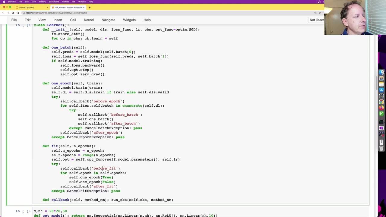
00:00:00.000 | Hi there and welcome to lesson 16 where we are working on building our first

00:00:07.840 | flexible training framework the learner and I've got some very good news which

00:00:14.640 | is that I have thought of a way of doing it a little bit more gradually and

00:00:19.400 | simply actually than last time so that should that should make things a bit

00:00:25.680 | easier so we're going to take it a bit more step by step so we're working in

00:00:30.080 | the 09 learner notebook today and we've seen already this this basic callbacks

00:00:43.480 | learner and so the idea is that we've seen so far this learner which wasn't

00:00:56.040 | flexible at all but it had all the basic pieces which is we've got a fit method

00:01:02.160 | we hard coding that we can only calculate accuracy and average loss we're

00:01:08.320 | hard coding we're putting things on a default device hard coding a single

00:01:14.760 | learning rate but the basic idea is here we go through each epoch and call one

00:01:20.280 | epoch to train or evaluate depending on this flag and then we loop through each

00:01:27.680 | batch in the data loader and one batch is going to grab the X and Y parts of

00:01:33.640 | the batch call the model call the loss function and if we're training do the

00:01:39.880 | backward pass and then print out we'll calculate the statistics for our

00:01:47.880 | accuracy and then at the end of an epoch print that out so it wasn't very

00:01:52.320 | flexible but it did do something so that's good so what we're going to do

00:01:58.760 | now is we're going to do is an intermediate step we're going to look at

00:02:01.400 | a but I'm calling a basic callbacks learner and it actually has nearly all

00:02:06.040 | the functionality of the full thing the way we're going to after we look at this

00:02:09.600 | basic callbacks learner we're then going to after creating some callbacks and

00:02:15.840 | metrics we're going to look at something called the flexible learner so let's go

00:02:20.000 | step by step so the basic callbacks learner looks very similar to the

00:02:26.680 | previous learner it it's got a fit function which is going to go through

00:02:36.880 | each epoch calling one epoch with training on and then training off and

00:02:43.520 | then one epoch will go through each batch and call one batch and one batch

00:02:52.480 | will call the model the loss function and if we're training it will do the

00:02:58.680 | backward step so that's all pretty similar but there's a few more things

00:03:03.160 | going on here for example if we have a look at fit you'll see that after

00:03:10.040 | creating the optimizer so we call self dot optfunk so optfunk here defaults to

00:03:18.840 | SGD so we instantiate an SGD object passing in our models parameters and

00:03:24.440 | the requested learning rate and then before we start looping through one

00:03:29.560 | epoch at a time now we've set epochs here we first of all call self dot

00:03:36.240 | callback and passing in before fit now what does that do self dot callback is

00:03:43.040 | here and it takes a method names in this case it's before fit and it calls a

00:03:49.440 | function called run callbacks it passes in a list of our callbacks and the

00:03:54.240 | method name in this case before fit so run callbacks is something that's going

00:04:01.120 | to go for each callback and it's going to sort them in order of their order

00:04:09.080 | attribute and so there's a base class through our callbacks which has an order

00:04:13.600 | of zero so our callbacks all going to have the same order of zero and which

00:04:16.720 | you will ask otherwise so here's an example of a callback so before we look

00:04:24.160 | at how callbacks work let's just let's just run a callback so we can create a

00:04:29.760 | ridiculously simple callback called completion callback which before we start

00:04:34.580 | fitting a new model it will set its count attribute to zero after each batch it

00:04:40.000 | will increment that and after completing the fitting process it will print out

00:04:44.960 | how many batches we've done so before we even train a model we could just run

00:04:49.200 | manually before fit after batch and after fit using this run cbs and you can

00:05:00.400 | see it's ended up saying completed one batches so what did that do so it went

00:05:06.880 | through each of the cbs in this list there's only one so it's going to look at

00:05:12.560 | the one cb and it's going to try to use get atra to find an attribute with this

00:05:20.320 | name which is before fit so if we try that manually so this is the kind of

00:05:26.360 | thing I want you to do if you find anything difficult to understand is do

00:05:29.520 | it all manually so create a callback set it to cbs zero just like you're doing in

00:05:34.880 | a loop right and then find out what happens if we call this and pass in this

00:05:47.240 | and you'll see it's returned a method and then what happens to that method it

00:05:55.680 | gets called so let's try calling it there yeah so that's what happened when

00:06:03.080 | we call the before fit which doesn't do anything very interesting but if we then

00:06:06.400 | call after batch and then we call after fit there it is right so yeah make sure

00:06:19.480 | you don't just run code really nearly but understand it by experimenting with

00:06:26.720 | it and I don't always experiment with it myself in these classes often I'm

00:06:30.400 | leaving that to you but sometimes I'm trying to give you a sense of how I

00:06:33.840 | would experiment with code if I was learning it so then having done that I

00:06:37.520 | would then go ahead and delete those cells but you can see I'm using this

00:06:40.520 | interactive notebook environment to to explore and learn and understand and so

00:06:48.160 | now we've got and if I haven't created a simple example of something to make it

00:06:53.260 | really easy to understand you should do that right don't just use what I've

00:06:56.440 | already created or what somebody else has already created so we've now got

00:07:00.160 | something that works totally independently we can see how it works

00:07:02.720 | this is what a callback does so a callback is something which will look at

00:07:07.320 | a class a callback is a class where you can define one or more of before after

00:07:14.720 | fit before after batch and before after epoch so it's going to go through and

00:07:23.040 | run all the callbacks that have a before fit method before we start fitting then

00:07:30.200 | it'll go through each epoch and call one epoch with training and one epoch with

00:07:34.780 | evaluation and then when that's all done it will call after fit callbacks and one

00:07:43.560 | epoch will before it starts on enumerating through the batches it will

00:07:51.120 | call before epoch and when it's done it will call after epoch the other thing

00:07:57.400 | you'll notice is that there's a try except immediately before every before

00:08:04.020 | method and immediately after every after method there's a try and there's an

00:08:09.320 | accept and each one has a different thing to look for cancel fit exception

00:08:13.320 | cancel epoch exception and cancel batch exception so here's the bit which goes

00:08:19.280 | through each batch calls before batch processes the batch calls after batch

00:08:24.480 | and if there's an exception that's of type cancel batch exception it gets

00:08:30.000 | ignored so what's that for so the reason we have this is that any of our

00:08:37.240 | callbacks could call could raise any one of these three exceptions to say I don't

00:08:48.200 | want to do this batch please so maybe you'll look an example of that in a

00:08:53.760 | moment so we can now train with this so let's call create a little get model

00:09:01.280 | function that creates a sequential model with just some linear layers and then

00:09:07.440 | we'll call fit and it's not telling us anything interesting because the only

00:09:11.900 | callback we added was the completion callback that's fine it's it's training

00:09:18.840 | it's doing something and we now have a trained model just didn't print out any

00:09:22.600 | metrics or anything because we don't have any callbacks for that that's the

00:09:25.720 | basic idea so we could create a maybe we could call it a single batch callback

00:09:38.760 | which after batch after a single batch it raises a cancel cancel fit exception

00:09:51.720 | so that's a pretty I mean that could be kind of useful actually if you want to

00:09:56.760 | just run one battery a model to make sure it works so we could try that so

00:10:07.680 | now we're going to add to our list of callbacks the single batch callback

00:10:14.320 | let's try it and in fact you know we probably want this let's just have a

00:10:22.920 | think here oh that's fine let's run it there we go so it ran and nothing

00:10:31.720 | happened and the reason nothing happened is because this canceled before this ran

00:10:39.280 | so we could make this run second by setting its order to be higher and we

00:10:45.800 | could say just order equals 1 because the default order is 0 and we sort in

00:10:52.920 | order of the order attribute actually let's use cancel epoch exception there

00:11:04.680 | we go that way it'll run the final fit there we are so it did one batch for the

00:11:15.240 | it did one batch for the training and one batch for the evaluation so it's a

00:11:21.000 | total of two batches so remember callbacks are not a special magic part

00:11:28.080 | of like the Python language or anything it's just a name we used refer to these

00:11:33.000 | functions or classes or callables more accurately that we that we pass into

00:11:39.880 | something that will then call back to that callable at particular times and I

00:11:45.540 | think these are kind of interesting kinds of callbacks because these

00:11:48.120 | callbacks have multiple methods in them so is each method a callback is each

00:11:54.840 | class with all those methods of callback I don't know I tend to think of the

00:11:58.020 | class with all the methods in as a single callback I'm not sure if we have

00:12:02.400 | great nomenclature for this all right so let's actually try to get this doing

00:12:08.680 | something more interesting by not modifying the learner at all but just by

00:12:11.680 | adding callbacks because that's the great hope of callbacks right so it

00:12:17.700 | would be very nice if it told us the accuracy and the loss so to do that it

00:12:24.520 | would be great to have a class that can keep track of a metric so I've created

00:12:29.440 | here a metric class and maybe before we look at it we'll see how it works you

00:12:37.600 | could create for example an accuracy metric by defining the calculation

00:12:42.600 | necessary to calculate the accuracy metric which is the mean of how often do

00:12:49.200 | the input sequence targets and the idea is you could then create an accuracy

00:12:53.960 | metric object you could add a batch of inputs and targets and add another batch

00:13:00.000 | of inputs and targets and get the value and there you would get the point four

00:13:06.960 | five accuracy or another way you could do it would be just to create a metric

00:13:13.080 | which simply takes gets the weighted average for example of your loss so you

00:13:16.640 | could add point six as the loss with a batch size of 32 point nine as a loss in

00:13:22.280 | a batch size of two and then that's going to give us a weighted average loss

00:13:28.000 | of point six two which is equal to this weighted average calculation so that's

00:13:34.240 | like one way we could kind of make it easy to calculate metrics so here's the

00:13:38.880 | class basically we're going to keep track of all of the actual values that

00:13:44.940 | we're averaging and the number in each mini batch and so when you add a mini

00:13:49.960 | batch we call calculate which for example for accuracy remember this is

00:13:56.800 | going to override the parent classes calculate so it does the calculation

00:14:01.520 | here and then we'll add that to our list of values we will add to our list of

00:14:08.680 | batch sizes the current batch size and then when you calculate the value we

00:14:16.480 | will calculate the weighted sum sorry the weighted mean weighted average now

00:14:24.320 | notice that here value I didn't have to put parentheses after it and that's

00:14:28.640 | because it's a property I think we've seen this before so just remind you

00:14:32.040 | property just means you don't have to put parentheses after it to get it's to

00:14:36.760 | get the calculation to happen all right so just let me know if anybody's got any

00:14:42.440 | questions up to here of course so we now need some way to use this metric in a

00:14:52.300 | callback to actually print out the first thing I'm going to do those are going to

00:14:56.160 | create one more one useful metric first a very simple one just two lines of code

00:15:01.080 | called the device callback and that is something which is going to allow us to

00:15:05.600 | use CUDA or for the Apple GPU or whatever without the complications we

00:15:14.880 | had before of you know how do we have multiple processes and our data loader

00:15:19.760 | and also use our device and not have everything fall over so the way we could

00:15:23.960 | do it is we could say before fit put the model onto the default device and before

00:15:34.600 | each batch is run put that batch onto the device because look what happened in

00:15:43.000 | in the this is really really important in the learner absolutely everything is

00:15:48.680 | put inside self dot which means it's all modifiable so we go for self dot

00:15:54.280 | iteration number comma self dot the batch itself enumerating the data loader

00:15:59.400 | and then we call one batch but before it we call the callback so we can modify

00:16:05.800 | this now how does the callback get access to the learner well what actually

00:16:11.520 | happens is we go through each of our call backs and put set an attribute

00:16:16.920 | called learn equal to the learner and so that means in the callback itself we can

00:16:23.720 | say self dot learn dot model and actually we could make this a bit better

00:16:29.000 | I think so make it like maybe you don't want to use a default device so this is

00:16:32.800 | where I would be inclined to add a constructor and set device and we could

00:16:38.840 | default it to the default device of course and then we could use that

00:16:47.560 | instead and that would give us a bit more flexibility so if you wanted to

00:16:51.480 | trade on some different device then you could I think that might be a slight

00:16:59.560 | improvement okay so there's a callback we can use to put things included and we

00:17:04.640 | could check that it works by just quickly going back to our old learner

00:17:09.120 | here remove the single batch CB and replace it with device CB yep still

00:17:23.560 | works so that's a good sign okay so now let's do our metrics now of course we

00:17:33.680 | couldn't use metrics until we built them by hand the good news is we don't have to

00:17:38.920 | write every single metric now by hand because they already exist in a fairly

00:17:43.480 | new project called torch eval which is an official PyTorch project and so torch

00:17:49.360 | eval is something that gives us actually I came across it after I had created my

00:17:56.200 | own metric class but it actually looks pretty similar to the one that I built

00:18:01.280 | earlier so you can install it with PEP I'm not sure if it's on Conde yet but

00:18:08.280 | it probably will be soon by the time you see the video I think it's pure of

00:18:12.080 | Python anyway so it doesn't matter how you install it and yeah it has a pretty

00:18:17.680 | similar pretty similar approach where you call dot update and you call dot

00:18:27.720 | compute so they're slightly different names but they're basically super

00:18:30.320 | similar to the thing that we just built but there's a nice good list of metrics

00:18:36.280 | to pick from so because we've already built our own now that means we're

00:18:41.280 | allowed to use theirs so we can import the multi-class accuracy metric and the

00:18:47.220 | main metric and just to show you they look very very similar if we call

00:18:53.200 | multi-class accuracy and we can pass in a mini batch of inputs and targets and

00:18:58.880 | compute and that all works nicely now these in fact it's exactly the same as

00:19:05.000 | what I wrote we both added this thing called reset which basically well resets

00:19:10.840 | it and it's obviously we're going to be wanting to do that probably at the start

00:19:15.880 | of each epoch and so if you reset it and then try to compute you'll get NAN

00:19:22.800 | because you can't get accuracy accuracies meaningless when you don't

00:19:26.560 | have any data yet okay so let's create a metrics callback so we can print out our

00:19:33.000 | metrics I've got some ideas to improve this which maybe I do this week but

00:19:37.980 | here's a basic working version slightly hacky but it's not too bad so generally

00:19:45.560 | speaking one thing I noticed actually is I don't know if this is considered a

00:19:49.540 | bug but a lot of the metrics didn't seem to work correctly and torch eval when I

00:19:54.600 | had tensors that were on the GPU and had requires grad so I created a little to

00:20:07.120 | CPU function which I think is very useful and that's just going to detach

00:20:12.720 | the so detach takes the tensor and removes all the gradient history the

00:20:17.800 | computation history used to calculate a gradient and puts it on the CPU that'll

00:20:22.760 | do the same for dictionaries of tensors lists of tensors and tuples of tensors

00:20:28.600 | so our metrics callback basically here's how we're going to use it so let's run

00:20:34.480 | it so here we're creating a metrics callback object and saying we want to

00:20:40.800 | create a metric called accuracy that's what's going to print out and this is

00:20:46.560 | the metrics object we're going to use to calculate accuracy and so then we just

00:20:51.400 | pass that in as one of our callbacks and so you can see what it's going to do is

00:20:57.880 | it's going to print out the epoch number whether it's training or evaluating so

00:21:03.560 | training set or validation set and it'll print out our metrics and our current

00:21:10.780 | status actually we can simplify that we don't need to print those bits because

00:21:18.000 | it's all in the dictionary now let's do that there we go um so let's take a look

00:21:30.640 | at how this works so we are going to be creating with for the callback we're

00:21:37.760 | going to be passing in the names and object metric objects for the metrics to

00:21:44.360 | track and print so here it is here star star metrics so he's seen star star

00:21:51.400 | before and as a little shortcut I decided that it might be nice if you

00:21:57.720 | didn't want to write accuracy equals you could just remove that and run it and if

00:22:04.440 | you do that then it will give it a name and I'll just use the same name as the

00:22:08.000 | class and so that's why you can either pass in so star ms will be a tuple well

00:22:15.280 | I mean it's got to be pulled out so it's just passing a list of positional

00:22:18.800 | arguments which we turn into a tuple or you can pass in named arguments that'll

00:22:23.560 | be turned into a dictionary if you pass in positional arguments then I'm going

00:22:27.560 | to turn them into named arguments in the dictionary by just grabbing the name

00:22:32.200 | from their type so that's where this comes from that's all that's going on

00:22:36.800 | here just a little shortcut bit of convenience so we store that away and

00:22:42.600 | this is yeah this is a bit I think I can simplify a little bit but I'm just

00:22:46.440 | adding manually an additional metric which is I'm going to call the loss and

00:22:51.760 | that's just going to be the weighted the weighted average of the losses so

00:22:57.480 | before we start fitting we we're going to actually tell the learner that we are

00:23:04.480 | the metrics callback and so you'll see later where we're going to actually use

00:23:08.320 | this before each epoch we will reset all of our metrics after each epoch we will

00:23:17.480 | create a dictionary of the keys and values which are the actual strings that

00:23:22.560 | we want to print out and we will call log which for now we'll just print them

00:23:28.840 | and then after each batch this is the key thing we're going to actually grab

00:23:34.880 | the input and target we're going to put them on the CPU and then we're going to

00:23:43.840 | go through each of our metrics and call that update so remember the update in

00:23:51.520 | the metric is the thing that actually says here's a batch of data right so

00:23:58.320 | we're passing in the batch of data which is the predictions and the targets and

00:24:04.200 | then we'll do the same thing for our special loss metric passing in the

00:24:09.320 | actual loss and the size of any batch and so that's how we're able to get this

00:24:17.720 | yeah this actual running on the Nvidia GPU and showing our metrics and obviously

00:24:26.720 | there's a lot of room to improve how this is displayed but all the

00:24:30.080 | informations we needed here and it's just a case of changing that function

00:24:35.560 | okay so that's our kind of like intermediate complexity learner we can

00:24:42.040 | make it more sophisticated but it's still exactly it's still going to fit in

00:24:48.800 | a single screen of codes this is kind of my goal here was to keep everything in a

00:24:51.920 | single screen of code this first bit is exactly the same as before but you'll see

00:24:59.360 | that the one epoch and fit and batch has gone from let's see but what it was

00:25:08.000 | before it's gone from quite a lot of code all this to much less code and the

00:25:19.680 | trick to doing that is I decided to use a context manager we're going to learn

00:25:23.240 | more about context managers in the next notebook but basically I originally last

00:25:27.600 | week I was saying I was going to do this as a decorator but I realized a context

00:25:30.080 | manager is better basically what we're going to do is we're going to call our

00:25:33.680 | before and after callbacks in a try accept block and to say that we want to

00:25:43.960 | use the callbacks in the try accept block we're going to use a with statement so

00:25:49.760 | in Python a with statement says everything in that block call our

00:25:56.680 | context manager before and after it now there's a few ways to do that but one

00:26:02.200 | really easy one is using this context manager decorator and everything up and

00:26:08.000 | to the up to the yield statement is called before your code where it says

00:26:13.440 | yield it then calls your code and then everything after the yield is called

00:26:18.760 | after your code so in this case it's going to be try self dot callback before

00:26:24.520 | name where name is fit and then it will call for self dot epoch etc because

00:26:34.280 | that's where the yield is and then it'll call self dot callback after fit

00:26:39.920 | accept okay and now we need to grab the cancel fit exception so all of the

00:26:48.320 | variables that you have in Python all live inside a special dictionary called

00:26:52.880 | globals so this dictionary contains all of your variables so I can just look up

00:26:57.320 | in that dictionary the variable called cancel fit with a capital F exception

00:27:04.480 | so this is except cancel fit exception so this is exactly the same then as this

00:27:12.160 | code except the nice thing is now I only have to write it once rather than at

00:27:18.080 | least three times and I'm probably going to want more of them so you know I tend

00:27:21.880 | to think it's worth yeah I tend to think it's worth refactoring a code when you

00:27:29.320 | have duplicate code particularly here we had the same code three times so that's

00:27:34.440 | going to be more of a maintenance headache we're probably going to want to

00:27:36.960 | add callbacks to more things later so by putting it into a context manager just

00:27:43.200 | once I think we're going to reduce our maintenance burden I know we do because

00:27:47.800 | I've had a similar thing in fast AI for some years now and it's been quite

00:27:51.760 | convenient so that's what this context managers about yeah other than that the

00:28:02.080 | code's exactly the same so we create our optimizer and then with our callback

00:28:06.960 | context manager for fit go through each epoch call one epoch set it to training

00:28:14.320 | or non training mode based on the argument we pass in grab the training or

00:28:19.600 | validation set based on the argument we trust in and then using the context

00:28:24.120 | manager for epoch go through each batch in the data loader and then for each

00:28:30.360 | batch in the data loader using the batch context now this is where something gets

00:28:37.500 | quite interesting we call predict get lost and if we're training backward step

00:28:43.000 | and zero grad but previously we actually called self dot model etc self dot loss

00:28:50.880 | function etc so we go through each batch and call before batch do the batch oh

00:29:05.680 | they say that's our that's our slow version wait what are we doing oh yes

00:29:11.720 | we're gonna be over here okay I'm back where we are yes so previously we were

00:29:25.480 | calling yeah calling calling the model calling the loss function calling loss

00:29:29.880 | dot backward opt dot step opt dot zero grad but now we are calling instead

00:29:40.280 | self dot predict self dot get lost self dot backward and how on earth is that

00:29:45.280 | working because they are not defined here at all and so the reason I've

00:29:49.800 | decided to do this is it gives us a lot of flexibility we can now actually create

00:29:55.240 | our own way of doing predict get lost backward step and zero grad in different

00:30:01.280 | situations and we're going to see some of those situations so what happens if

00:30:09.400 | we call self dot predict and it doesn't exist well it doesn't necessarily cause

00:30:14.240 | an error what actually happens is it calls a special magic method in Python

00:30:19.840 | called dunder get atra as we've seen before and what I'm doing here is I'm

00:30:24.840 | saying okay well if it's one of these special five things don't raise an

00:30:29.680 | attribute error which is this is the default thing it does but instead create

00:30:36.800 | a call back or actually I should say call self dot call back passing in that

00:30:43.840 | name so it's actually going to call self dot call back quote predict and self dot

00:30:51.480 | call back is exactly the same as before and so what that means now is to make

00:30:55.200 | this work exactly the same as it did before I need a call back which does

00:30:59.260 | these five things and here it is I'm going to call it train call back so here

00:31:05.640 | are the five things predict get lost backwards step and zero grad so there

00:31:10.760 | are here predict get lost backwards step and zero grad okay so they're almost

00:31:23.760 | exactly the same as what they looked like in our intermediate learner except

00:31:27.560 | now I just need to have self dot learn in front of everything because we

00:31:31.320 | remember this is a callback it's not the learner and so for a callback the

00:31:35.000 | callback can access the learner using self dot learn so self dot learn dot

00:31:38.040 | preds is self dot learn dot model passing in self dot learn dot batch and

00:31:42.040 | just the independent variables ditto for the loss calls the loss function

00:31:48.180 | backward step zero grad so that's at this point this isn't doing anything that

00:31:58.160 | wasn't doing before but the nice thing is now if you want to use hugging face

00:32:03.400 | accelerate or you want something that works on hugging face data styles

00:32:07.320 | dictionary things or whatever you can actually change exactly how it behaves

00:32:14.400 | by just call passing by creating a callback for training and if you want

00:32:20.260 | everything except one thing to be the same you can inherit from train CB so

00:32:23.760 | this is I've I've not tried this before I haven't seen this done anywhere else

00:32:28.280 | so it's a bit of an experiment so I would sit here how you go with it and then

00:32:34.520 | finally I thought it'd be nice to have a progress bar so let's create a progress

00:32:38.720 | callback and the progress bar is going to show on it our current loss and going to

00:32:44.600 | put create a plot of it so I'm going to use a project that we created called

00:32:52.160 | fast progress mainly created by the wonderful Sylvain and basically fast

00:33:02.400 | progress is yeah very nice way to create a very flexible progress bars and so let

00:33:10.760 | me show you what it looks like first so let's get the model and train and as you

00:33:15.520 | can see it actually in real time updates the graph and everything there you go

00:33:21.240 | that's pretty cool so that's the that's the progress bar the metrics callback the

00:33:27.720 | device callback and the training callback all in action so before we fit we

00:33:33.720 | actually have to set self dot learn dot epochs now that might look a little bit

00:33:39.960 | weird but self dot learn dot epochs is the thing that we loop through for self

00:33:46.800 | dot epoch in so we can change that so it's not just a normal range but instead

00:33:52.280 | it is a progress bar around a range we can then check remember I told you that

00:34:01.080 | the learner is going to have the metrics attribute applied we can then say oh if

00:34:04.400 | the learner has a metrics attribute then let's replace the underscore log method

00:34:11.000 | there with ours and our one instead will write to the progress bar now this is

00:34:17.460 | pretty simple it looks very similar to before but we could easily replace this

00:34:21.000 | for example with something that creates an HTML table which is another thing

00:34:24.840 | fast progress does or other stuff like that so you can see we can modify the

00:34:29.520 | nice thing is we can modify how our metrics are displayed so that's a very

00:34:35.080 | powerful thing that Python lets us do is actually replace one piece of code with

00:34:38.960 | another and that's the whole purpose of why the metrics callback had this

00:34:46.760 | underscore log separately so why didn't I just say print here that's because this

00:34:51.800 | way classes can replace how the metrics are displayed so we could change that to

00:34:58.340 | like send them over to weights and biases for example or you know create

00:35:03.800 | visualizations or so forth so before epoch we do a very similar thing the

00:35:12.480 | self dot learn dot DL iterator we change it to have a progress bar wrapped around

00:35:17.400 | it and then after each bar we set the progress bars comment to be the to be the

00:35:26.240 | loss it's going to print just going to show the loss on the progress bar as it

00:35:29.320 | goes and if we've asked for a plot then we will append the losses to a list of

00:35:36.040 | losses and we will update the graph with the losses and the batch numbers so

00:35:51.200 | there we have it we have a yeah nice working learner which is I think the most

00:36:00.640 | flexible learner that training loop probably that's I hope has ever been

00:36:05.080 | written because I think the fast AI 2 one was the most flexible that had ever

00:36:08.880 | been written before and this is more flexible and the nice thing is you can

00:36:14.400 | make this your own you know you can you know fully understand this training loop

00:36:20.760 | so it's kind of like you can use a framework but it's a framework in which

00:36:25.720 | you're totally in control of it and you can make it work exactly how you want to

00:36:29.280 | ideally not by changing the change in the learner itself ideally by creating

00:36:33.880 | callbacks but if you want to you could certainly like look at that the whole

00:36:38.000 | learner fits on a single screen so you could certainly change that we haven't

00:36:44.320 | added inference yet although that shouldn't be too much to add I guess we

00:36:47.880 | have to do that at some point okay now interestingly I love this about Python

00:36:55.440 | it's so flexible when when we said self dot predict self dot get lost I said if

00:37:03.500 | they don't exist then it's going to use get atcha and it's going to try to find

00:37:08.440 | those in the callbacks and in fact you could have multiple callbacks that define

00:37:14.420 | these things and then they would chain them together which would be kind of

00:37:17.040 | interesting but there's another way we could make these exist which is which is

00:37:24.520 | that we could subclass this so let's not use train CB just to just to show us how

00:37:30.840 | this would work and instead we're going to use a subclass so here in a subclass

00:37:38.040 | learner and I'm going to override the five well it's not exactly overriding I

00:37:43.680 | didn't have any definition of them before so I'm going to define the five

00:37:46.200 | directly in the learner subclass so that way it's never going to end up going to

00:37:50.640 | get atcha because get atcha is only called if something doesn't exist so

00:38:02.160 | here it's basically all these five are exactly the same as in our train

00:38:07.440 | callback except we don't need self dot learn anymore we can just use self

00:38:10.560 | because we're now in the learner but I've changed zero grad to do something a

00:38:15.120 | bit crazy I'm not sure if this has been done before I haven't seen it but maybe

00:38:20.120 | it's an old trick that I just haven't come across but it occurred to me zero

00:38:24.680 | grad which remember is the thing that we call after we take the optimizer step

00:38:30.240 | doesn't actually have to zero the gradients at all what if instead of

00:38:35.240 | zeroing the gradients we multiplied them by some number like say 0.85 well what

00:38:47.360 | would that do well what it would do is it would mean that your previous

00:38:53.080 | gradients would still be there but they would be reduced a bit and remember what

00:39:00.680 | happens in PyTorch is PyTorch always adds the gradients to the existing

00:39:07.100 | gradients and that's why we normally have to call zero grad but if instead we

00:39:12.160 | multiply the gradients by some number I mean we should really make this a

00:39:15.600 | parameter let's do that shall we so let's create a parameter so probably the

00:39:25.840 | few ways we could do this well let's do it properly we've got a little bit of

00:39:34.960 | time so we could say well maybe just copy and paste all those over here and

00:39:51.000 | we'll add momentum momentum equals 0.85 self momentum equals momentum and then

00:40:08.200 | super so make sure you call the super classes passing in all the stuff we

00:40:18.480 | could use delegates for this and quags that would be possibly another great way

00:40:22.400 | of doing it but let's just do this for now okay and then so there we wouldn't

00:40:27.480 | make it 0.85 we would make it self dot momentum so you'll see now still trains

00:40:35.560 | but there's no train CB callback anymore in my list I don't need one because I

00:40:41.880 | have to find the five methods in the subclass now this training at the same

00:40:47.800 | learning rate for the same time the accuracy it improves by more let's run

00:40:54.100 | them all yeah this is a lot like gradient accumulation callback they're

00:41:02.080 | kind of cooler I think okay so the let's see the loss has gone from 0.8 to 0.55

00:41:16.480 | and the accuracy is gone from about 0.7 to about 0.8 so they've improved why is

00:41:24.400 | that well we're going to be learning a lot more about this pretty shortly but

00:41:32.220 | basically what's happening here but basically what's happening here is we

00:41:40.600 | have just implemented in a very interesting way which I haven't seen done

00:41:44.160 | before something called momentum and basically what momentum does is it say

00:41:49.200 | like imagine you are you know you're trying you've got some kind of complex

00:41:55.240 | contour lost surface right and you know so imagine these are hills with a marble

00:42:05.880 | very similar right and your marbles up here what would normally happen with

00:42:10.920 | gradient descent is it would go you know in the direction downhill which is this

00:42:16.960 | way so we'll go whoa over here and then whoa over here right very slow what

00:42:23.880 | momentum does is it's is the first steps the same and then the second step says oh

00:42:29.160 | I wanted to go this way but I'm going to add together the previous direction plus

00:42:35.280 | the new direction but reduce the previous direction a bit so that would

00:42:38.800 | actually make me end up about here and then the second one does the same thing

00:42:44.560 | and so momentum basically makes you much more quickly go to your destination so

00:42:52.600 | normally momentum is done it the reason I did it this way partly to show you is

00:42:57.100 | just a bit of fun a bit of interest but it's very it's very useful because

00:43:00.940 | normally momentum you have to store a complete copy basically of all the

00:43:05.800 | gradients the momentum version of the gradients so that you can kind of keep

00:43:10.080 | track of that that that running exponentially weighted moving average but

00:43:14.320 | using this trick you're actually using the dot grad themselves to store the

00:43:20.680 | exponentially weighted moving average so anyway there's a little bit of fun which

00:43:25.440 | hopefully particularly those of you who are interested in accelerated optimizers

00:43:31.360 | and memory saving might find a bit inspiring all right there's one more

00:43:40.220 | call back I'm going to show before the break which is the wonderful learning

00:43:46.200 | ratefinder I'm assuming that anybody who's watching this already is familiar

00:43:50.760 | with the learning ratefinder from fast AI if you're not there's lots of videos

00:43:55.760 | and tutorials around about it it's an idea that comes from a paper by Leslie

00:44:01.300 | Smith from a few years ago and the basic idea is that we will increase the

00:44:08.640 | learning rate I should have put titles on this the the x-axis here is learning

00:44:12.320 | rate the y-axis here is loss we increase the learning rate gradually over time

00:44:19.320 | and we plot the loss against the learning rate and we find how high can

00:44:24.940 | we bring the learning rate up before the loss starts getting worse you kind of

00:44:30.160 | want roughly where about the steepest slope is so probably here it would be

00:44:34.060 | about 0.1 so it'd be nice to create a learning ratefinder so here's a

00:44:41.200 | learning ratefinder callback so what a learning ratefinder needs to do well you

00:44:46.720 | have to tell it how much to multiply the learning rate by each batch let's say we

00:44:50.440 | add 30% to the learning rate each batch and so we'll store that so before we fit

00:44:55.920 | we obviously need to keep track of the learning rates and we need to keep track

00:45:00.040 | of the losses because those are the things that we put on a plot the other

00:45:05.800 | thing we have to do is decide when do we stop training so when is it clearly gone

00:45:10.120 | off the rails and I decided that if the loss is three times higher than the

00:45:16.200 | minimum loss we've seen then we should stop so we're going to keep track of

00:45:20.520 | their minimum loss and so let's just initially set that to infinity it's a

00:45:25.340 | nice big number well not quite a number but a number ish like thing so then

00:45:31.360 | after every batch first of all let's check that we're training okay if we're

00:45:35.200 | not training then we don't want to do anything we don't use the learning rate

00:45:39.480 | finder during validation so here's a really handy thing just raise cancel

00:45:43.680 | epoch exception and that stops it from doing that epoch entirely so just to see

00:45:49.220 | how that works you can see here one epoch does with the call back context

00:45:58.120 | manager epoch and that will say oh it's got cancelled so it goes straight to the

00:46:04.000 | accept which is going to go all the way to the end of that code and it's going

00:46:09.640 | to skip it so it's you can see that we're using exceptions as control

00:46:14.960 | structures which is actually a really powerful programming technique that is

00:46:24.000 | really underutilized in my opinion like a lot of things I do it's actually

00:46:29.280 | somewhat controversial some people think it's a bad idea but I find it actually

00:46:35.480 | makes my code more concise and more maintainable and more powerful so I like

00:46:40.920 | it so let's see yeah so that's we've got our cancel epoch exception so then we're

00:46:49.980 | just going to keep track of our learning rates the learning rates we're going to

00:46:54.200 | learn a lot more about optimizers shortly so I won't worry too much about

00:46:57.280 | this but basically the learning rates are stored by PyTorch inside the

00:47:01.020 | optimizer and they're actually stored in things called param groups parameter

00:47:04.400 | groups so don't worry too much about the details but we can grab the learning

00:47:08.240 | rate from that dictionary and we'll learn more about that shortly we've got

00:47:12.480 | to keep track of the loss appended to our list of losses and if it's less than

00:47:17.320 | the minimum we've seen then recorded as the minimum and if it's greater than a

00:47:22.000 | three times the minimum then look at this it's really cool cancel fit

00:47:25.240 | exception so this will stop everything in a very nice clean way no need for lots

00:47:35.520 | of returns and conditionals or and stuff like that just raise the cancel fit

00:47:39.760 | exception and yeah and then finally we've got to actually update our learning

00:47:47.920 | rate to 1.3 times the previous one and so basically the way you do it in PyTorch

00:47:54.080 | is you have to go through each parameter group and grab the learning rate in the

00:47:58.160 | dictionary and multiply it by lrmult so yeah you've already seen it run and we

00:48:05.480 | can at the end of running you will find that there is now a the callback will

00:48:12.280 | now contain an LR's and a losses so for this callback I can't just add it

00:48:17.600 | directly to the callback list I need to instantiate it first and the reason I

00:48:22.780 | need to instantiate it first is because I need to be able to grab its learning

00:48:25.800 | rates and its losses and in fact you know we could grab that whole thing and

00:48:30.280 | move it in here there's no reason callbacks only have to have the callback

00:48:34.120 | things right so we could do this and now that's just going to become self there

00:48:50.280 | we go and so then we can train it again and we could just call LR find dot plot

00:48:57.440 | so callbacks can really be you know quite self-contained nice things as you

00:49:03.640 | can see so there's a more sophisticated callback and I think it's doing a lot of

00:49:08.080 | really nice stuff here you might have come across something in PyTorch called

00:49:14.880 | learning rate schedulers and in fact we could implement this whole thing with a

00:49:20.360 | learning rate scheduler it won't actually save that much time but I just

00:49:24.160 | want to show you when you use stuff in PyTorch like learning rate schedulers

00:49:28.400 | you're actually using things that are extremely simple the learning rate

00:49:31.720 | scheduler basically does this one line of code for us so I'm going to now create a

00:49:35.960 | new LR find a CB and this time I'm going to use the PyTorch's exponential LR

00:49:42.880 | scheduler which is here so this is now it's interesting that actually the

00:49:51.560 | documentation of this is kind of actually wrong it claims that it decays

00:49:56.600 | the learning rate of each parameter group by gamma so gamma is just some

00:50:00.320 | number you pass in I don't know why this has to be a Greek letter but it sounds

00:50:04.600 | more fancy than multiplying by an LR multiplier it says every epoch but it's

00:50:11.080 | not actually done every epoch at all what actually happens is in PyTorch the

00:50:17.560 | schedulers have a step method and the decay happens each time you call step

00:50:23.240 | and if you set gamma which is actually LR mult to a number bigger than one it's

00:50:29.300 | not a decay it's an increase so the difference now I guess I'll copy and

00:50:34.400 | paste the previous version okay so the previous versions on the top so the main

00:50:43.520 | difference here is that before fit we're going to create something called a self

00:50:47.360 | dot shed equal to the scheduler and the scheduler because it's going to be

00:50:53.300 | adjusting the learning rates it actually needs access to the optimizer so we pass

00:50:56.760 | in the optimizer and the learning rate model player and so then in after batch

00:51:04.200 | rather than having this line of code we replace it with this line of code self

00:51:09.320 | dot shed dot step so that's the only difference and you know I mean we're not

00:51:14.040 | gaining much as I said by using the PyTorch exponential LR scheduler but I

00:51:20.040 | mainly wanted to do it so you can see that these things like PyTorch

00:51:23.440 | schedulers are not doing anything magic they're just doing that one line of code

00:51:27.960 | for us and so I run it again using this new version oopsy dozy oh I forgot to

00:51:36.880 | run this line of code there we go and I guess I should also add the nice little

00:51:44.920 | plot method maybe we'll just move it to the bottom there

00:51:54.720 | lrfind dot plot there we go and put that one back to how it was all right perfect

00:52:09.520 | timing so we added a few very important things in here so make sure we export

00:52:14.820 | and we'll be able to use them shortly all right let's have an eight minute break

00:52:23.120 | it's just have a 10 minute break so I see you back here at um eight past all

00:52:33.400 | right welcome back um one suggestion which I lately like is we could rename

00:52:37.320 | plot to after fit which I really like because that means we should be able to

00:52:47.520 | then just call learn dot fit and delete the next one and let's see it didn't

00:52:54.520 | work why not oh no that doesn't work does it because the hmm you know what I

00:53:07.200 | think the callback here could go into a finally block actually that would

00:53:19.600 | actually allow us to always call the callback even if we've cancelled I think

00:53:26.400 | that's reasonable that might have its own confusions anyway we could try it

00:53:31.640 | for now because that would let us put this after fit in there we go so that

00:53:41.760 | automatically runs then so that's an interesting idea I think I quite like it

00:53:56.040 | cool so let's now look at notebook 10 so I feel like this is the the next big

00:54:06.640 | piece we need so we've got a pretty good system now for training models what I

00:54:14.600 | think we're really missing though is a way to identify how our models are

00:54:20.080 | training and so try identify how our models are training we need to be able

00:54:24.880 | to look inside them and see what's going on while they train we don't currently

00:54:29.080 | have any way to do that and therefore it's very hard for us to diagnose and

00:54:34.360 | fix problems most people have no way of looking inside their models and so most

00:54:39.280 | people have no way to properly diagnose and fix models and that's why most

00:54:42.920 | people when they have a problem with training their model randomly try things

00:54:46.200 | until something starts hopefully working we're not going to do that we're going

00:54:50.920 | to do it properly so we can import the stuff that we just created in the

00:54:56.320 | learner and the first thing I'm going to do introduce now is a set seed function

00:55:02.440 | we've been using torch manual seed before we know all about RNGs random

00:55:08.360 | number generators we've actually got three of them pie torches numpies and

00:55:14.640 | pythons let's see all of them and also in python pytorch you can use a flag to

00:55:22.520 | ask it to use deterministic algorithms so things should be reproducible as we

00:55:26.840 | discussed before you shouldn't always just make things reproducible but for

00:55:30.720 | lessons I think this is useful so here's a function that lets you set a

00:55:35.000 | reproducible seed all right let's use the same data set as before a fashion

00:55:39.440 | MNIST data set will load it up in the same way and let's create a model that

00:55:45.440 | looks very similar to our previous models this one might be a bit bigger

00:55:49.400 | might not I didn't actually check okay so let's use multiclass accuracy again

00:55:59.000 | same callbacks that we used before we'll use the train CB version for no

00:56:04.200 | particular reason and generally speaking we want to train as fast as possible not

00:56:12.480 | just because we don't like wasting time but actually more importantly because

00:56:16.240 | the fact the higher the learning rate you train at the more the more you're

00:56:20.800 | able to find a often more generalizable set of weights and also oh training

00:56:35.080 | quickly also means that we can look at each batch let each item in the data

00:56:40.880 | less often so we're going to have less issues with overfitting and generally

00:56:44.880 | speaking being if we can train at a high learning rate then that means that we're

00:56:49.200 | learning to train in a stable way and stable training is is very good so let's

00:56:56.840 | try setting up a high learning rate of point six and see what happens so here's

00:57:02.600 | a function that's just going to create a learner with our callbacks and fit it

00:57:07.600 | and return the learner in case we want to use it and it's training oh and then

00:57:14.320 | it suddenly fell apart so it's going well for a while and then it stopped

00:57:19.000 | training nicely so one nice thing about this graph is that we can immediately

00:57:22.640 | see when it stops training well which is very useful so what happened there why

00:57:30.960 | did it go badly I mean we can guess that it might have been because of our high

00:57:33.760 | learning rate but what's really going on so let's try to look inside it so one

00:57:39.440 | way to look inside it would be we could create our own sequential model which

00:57:46.040 | just like the sequential model we've built before with do you remember we

00:57:49.920 | created one using nn.module list in a previous lesson if you've forgotten go

00:57:54.160 | back and check that out and when we call that model we go through each layer and

00:58:01.840 | just call the layer and what we could do is though we could add something in

00:58:07.120 | addition which is at each layer we could also get the mean of that layer and the

00:58:17.280 | standard deviation of that layer and append them to a couple of different

00:58:25.000 | lists and activation means and activation standard deviations this is

00:58:29.240 | going to contain after we call this model it's going to contain the means

00:58:34.560 | and standard deviations for each layer and then we could define dunder iter

00:58:42.280 | which makes this into an iterator as being let's say just oh just it when you

00:58:46.400 | iterate through this model you can iterate through the layers so we can

00:58:52.400 | then train this model in the usual way and this is going to give us exactly the

00:58:56.080 | same outcome as before because I'm using the same seed so you can see it looks

00:58:59.440 | identical but the difference is instead of using nn.sequential we've now

00:59:05.080 | used something that's actually saved the means and standard deviations of each

00:59:08.600 | layer and so therefore we can plot them okay so here we've plotted the

00:59:20.240 | activation means and notice that we've done it for every batch so that's why

00:59:27.880 | along the x-axis here we have batch number and on the y-axis we have the

00:59:32.520 | activation means and then we have it for each layer so rather than starting at one

00:59:37.160 | because we play from starting at zero so this is the first layer is blue second

00:59:40.960 | layer is orange third layer green fourth layer red and fifth layer watch for that

00:59:48.600 | like movie kind of color and look what's happened the activations have started

00:59:57.200 | pretty small close to zero and have increased at an exponentially increasing

01:00:01.640 | rate and then have crashed and then have increased again an exponential rate and

01:00:07.280 | crashed again it increased again crashed again and each time they've not gone up

01:00:12.160 | they've gone up even higher and they've crashed in this case even lower and what

01:00:18.040 | happens well wait what's happening here when our activations are really close to

01:00:22.040 | zero well when your activations are really close to zero that means that the

01:00:26.200 | inputs to each layer are numbers very close to zero as a result of which of

01:00:31.680 | course the outputs are very close to zero because we're doing just matrix

01:00:36.000 | multiplies and so this is a disaster when activations are very close to zero

01:00:41.920 | you're there there they're dead units they're not able to do anything and you

01:00:47.880 | can see for ages here it's not training at all and this is so this is the this

01:00:52.680 | is the activation means the standard deviations tell an even stronger story

01:00:55.880 | so you want generally speaking you want the means of the activations to be about

01:01:03.400 | zero and the standard deviations to be about one mean of zero is fine as long

01:01:09.720 | as they're spread around zero but a standard deviation of close to zero is

01:01:14.120 | terrible because that means all of the activations are about the same so here

01:01:18.760 | after batch 30 all all of the activations are close to zero and all of

01:01:24.600 | their standard deviations are close to zero so all the numbers are about the

01:01:27.680 | same and they're about zero so nothing's going on and you can see the same things

01:01:33.560 | happening with standard deviations we start with not very much variety in the

01:01:37.220 | weights it exponentially increases how much variety there is and then it crashes

01:01:41.200 | again exponentially increases crashes again this is a classic shape of bad

01:01:48.080 | behavior and with these two plots you can really understand what's going on in

01:01:55.200 | your model and if you train a model and at the end of it you kind of think well

01:02:00.200 | I wonder if this is any good if you haven't looked at this plot you don't

01:02:03.800 | know because you haven't checked to see whether it's training nicely maybe it

01:02:07.920 | could it could be a lot better if you can get something we'll see some nicer

01:02:12.240 | training pictures later but generally speaking you want something where your

01:02:16.560 | main is always about zero and your variance is always about one standard

01:02:21.880 | deviation is always about one and if you see that then it's a pretty good chance

01:02:26.840 | you're training properly if you don't see that you're most certainly not

01:02:30.160 | training properly okay so what I'm going to do in the rest of this part of the

01:02:34.800 | lesson is explain how to do this in a more elegant way because as I say being

01:02:40.800 | able to look inside your models is such a critically important thing to building

01:02:45.240 | and debugging models we don't have to do it manually we don't have to create our

01:02:49.440 | own sequential model we can actually use a pytorch thing called hooks so as it

01:02:55.680 | says here a hook is called when a layer that it's registered to is executed

01:03:00.920 | during the forward pass that's quite a forward hook well the backward pass and

01:03:04.880 | that's called a backward hook and so the key thing about hooks is we don't have

01:03:08.280 | to rewrite the model we can add them to any existing model so we can just use

01:03:13.320 | standard nn.sequential passing in our layers which were these ones here and so

01:03:23.840 | we're still going to have something to keep track of the activation means and

01:03:26.720 | standard deviation so just create an empty list for now for each layer in the

01:03:31.940 | model and let's create a little function it's going to be called because a hawk

01:03:38.040 | is going to call a function when when during the forward pass for a forward

01:03:43.040 | hook or the backward pass or a backward hook so it could have function called a

01:03:46.160 | pen stats it's going to be passed the hook number sorry the layer number the

01:03:51.440 | module and the input and the output so we're going to be grabbing the outputs

01:03:58.240 | mean and putting in in activation means and the output standard deviation and

01:04:02.600 | putting it in activation standard deviations so here's how you do it we've

01:04:07.440 | got a model you go through each layer of the model and you call on it register

01:04:13.120 | forward hook that's part of pytorch and we don't need to write it ourselves

01:04:16.960 | because we already did right it's just doing the same thing as this basically

01:04:20.240 | and what function is always going to be called the function that's going to be

01:04:28.240 | called is the append stats function passing in remember partial is the

01:04:33.760 | equivalent of saying a pen stats passing in I as the first element the first

01:04:38.940 | argument so if we now fit that model it trains in the usual way but after each

01:04:46.600 | after each layer it's going to call this and so you can see we get exactly the

01:04:54.120 | same thing as before so one question we get here is what's the difference

01:04:58.680 | between a hook and a callback nothing at all hooks and call backs are the same

01:05:03.740 | thing it's just that pytorch defines hooks and they call them hooks instead

01:05:09.800 | of callbacks they are less flexible than the callbacks that we used in in the

01:05:18.920 | learner because you don't have access to all the available states you can't

01:05:22.400 | change things but there are you know there are particular kind of callback

01:05:26.000 | it's just setting a piece of code that's going to be run for us when we when

01:05:33.620 | something happens and in this case there's something that happens is that

01:05:36.400 | either layer in the forward pass is called or a layer in the backward pass

01:05:39.800 | is called I guess you could describe the function that's being called back as the

01:05:47.180 | callback and the thing that's doing the callback has the hook I'm not sure if

01:05:52.560 | that level of distinction is important but maybe that's you could do that okay

01:05:57.320 | so anyway this is a little bit fussy of kind of like creating globals and

01:06:02.080 | depending to them and stuff like that so let's try to simplify this a little bit

01:06:06.160 | so what I did here was I created a class called hook so this class when we create

01:06:15.760 | it we're going to pass in the module that we're hooking so we call M dot

01:06:22.160 | register forward hook and we call the function we pass the function that we

01:06:26.280 | want to be given and so here's the pass the function and we're also going to

01:06:31.080 | pass in the hook class to the function let's also define a remove because this

01:06:41.540 | is actually the thing that this is actually the thing that removes the hook

01:06:46.120 | we don't want it sitting around forever this is called the Dell is called by

01:06:52.080 | Python when an object is freed so when that happens we should also make sure

01:06:56.720 | that we remove this okay so appends that's now we're going to replace it's

01:07:05.120 | going to instead get past the hook instead because that's what we asked to

01:07:13.700 | be passed and if there's no dot stats attribute in there yet then let's

01:07:21.980 | create one and then we're going to be past the activation so put that on the

01:07:29.780 | CPU and append the mean and at the standard deviation and now the nice thing

01:07:35.060 | is that the stats are actually inside this object which is convenient so now

01:07:40.480 | we can do exactly the same thing as before but we don't have to set any of

01:07:44.560 | that global stuff or whatever we can just say okay our hooks is a hook with

01:07:49.440 | that layer and that function for all those models layers and so we're just

01:07:58.640 | calling it has called register forward hook for us so now when we fit that it's

01:08:05.960 | going to run with the hooks there we go it trains actually they did do it too

01:08:22.800 | okay so then it trains and we get exactly the same shape as usual and we

01:08:33.120 | get back the same results as usual but as we can see we're gradually making

01:08:35.920 | this more convenient which is nice so we can make it nicer still because

01:08:44.760 | generally speaking we're going to be adding multiple hooks and this stuff of

01:08:48.880 | you know this list comprehension whatever it's a bit inconvenient so

01:08:52.800 | let's create a hooks class so first of all we'll see how the hooks class works

01:08:57.520 | in practice so in the hooks class the way we're going to use it is we're going

01:09:02.520 | to call with hooks pass in the model pass in the function to use as their hook

01:09:09.920 | and then we'll fit the model and that's it it's going to be literally just one

01:09:15.000 | extra line of code to set up the whole thing and then when we then you can then

01:09:19.360 | go through each hook and plot the main and standard deviation of each layer so

01:09:25.180 | that's how that's the hooks class is going to make things much easier so the

01:09:29.020 | hooks class as you can see we're using a making it a context manager and we want

01:09:38.640 | to be able to loop through it we want to be an index into it so it's quite a lot

01:09:43.200 | of behavior we want believe it or not all that behavior is in this tiny little

01:09:48.040 | thing and we're going to use the most flexible general way of creating context

01:09:54.360 | managers now context managers are things that we can say with the general way of

01:09:58.960 | creating a context manager is to create a class and to find two special things

01:10:03.560 | done to enter and done to exit done to enter is a function that's going to be

01:10:08.600 | called when it hits the with statement and if you add an as blah after it then

01:10:16.440 | the contents of this variable will be whatever is returned from done to enter

01:10:21.600 | and as you can see we just return the object itself so the the hooks object is

01:10:27.240 | going to be stored in hooks now interestingly the hooks class inherits

01:10:35.440 | from list you can do this you can actually inherit from stuff like list in

01:10:39.660 | python so a hooks the hooks object is a list and therefore we need to call the

01:10:45.360 | super classes constructor and we're going to pass in a that list comprehension we

01:10:51.120 | saw that list of hooks where it's going to hook into each module in the list of

01:10:56.480 | modules we asked to hook into now we're passing in a model here but because the

01:11:04.280 | model is an nn dot sequential you can actually loop through an nn dot

01:11:07.640 | sequential and it returns each of the layers so this is actually very very

01:11:12.080 | nice and concise and convenient so that's the constructor done to enter just

01:11:18.000 | returns it done to exit is what's called automatically at the end of the whole

01:11:24.360 | block so when this whole thing's finished it's going to remove the hooks

01:11:29.440 | and removing the hooks is just going to go through each hook and remove it the

01:11:34.760 | reason we can do for H and self is because remember this is a list and then

01:11:43.560 | finally we've got a dunder dell like before and I also added a dunder dell

01:11:48.840 | item this is the thing that lets you delete a single hook from the list which

01:11:53.280 | will remove that one hook and call the list still item so there's our whole

01:12:01.640 | thing so this is going to this this this one's optional this is the one that lets

01:12:05.000 | us remove a single hook rather than all of them so let's just understand some of

01:12:12.200 | what's going on there so here's a dummy context manager as you can see here it's

01:12:18.240 | got a dunder enter which is going to return itself and it's going to print

01:12:22.960 | something so you can see here I call with dummy context manager and so

01:12:28.400 | therefore it prints let's go first the second thing it's going to do is call

01:12:34.120 | this code inside the context manager so we've got as DCM so that's itself and

01:12:40.640 | so it's gonna call hello which prints hello so here it is and then finally

01:12:48.160 | it's going to automatically call exit dunder exit which is all done so here's

01:12:53.920 | all done so again if you haven't used context managers before you want to be

01:12:58.160 | creating little samples like this yourself and getting them to work so

01:13:02.120 | this is your key homework for this week is anything in the lesson where we're

01:13:09.160 | using a part of Python you're not a hundred percent familiar with is for you

01:13:13.280 | to from scratch to create some simple like kind of dummy version that fully

01:13:18.480 | explores what it's doing if you're familiar with all the Python pieces then

01:13:24.080 | it's to create your own you know that is to explore do the same thing with the

01:13:29.000 | PyTorch pieces like with with hooks and so forth and so I just wanted to show

01:13:35.640 | you also what it's like to inherit from list so here I'm here inheriting from a

01:13:40.120 | list and I could redefine how dunder Dell item works so now I can create a

01:13:46.000 | dummy list and it looks exactly the same as usual but now if I delete an item

01:13:54.040 | from the list it's going to call my overridden version and then it will

01:14:01.680 | call the original version and so the list is now got removed that item and did

01:14:06.840 | this at the same time so you can see you can actually yeah modify how Python

01:14:11.360 | works or create your own things that get all the behavior or the convenience of

01:14:16.720 | Python classes like this one and add stuff to them so that's what's happening

01:14:22.600 | there okay so that's our hooks class so the next bit was developed largely

01:14:34.600 | developed the last time I think it was that we did a part 2 course in San

01:14:39.520 | Francisco with Stefano so many thanks to him for helping get this next bit

01:14:44.000 | looking great we're going to create my favorite single image explanations of

01:14:52.040 | what's going on inside a model we call them the colorful dimension which they're

01:14:58.160 | histograms we're going to take our same append stats these are all the same as

01:15:04.080 | before we're going to add an extra line of code which is to get a histogram of

01:15:09.040 | the absolute values of the activations so a histogram a histogram to remind

01:15:15.600 | you is something that takes a collection of numbers and tells you how

01:15:21.680 | frequent each group of numbers are and we're going to create 50 bins for our

01:15:28.640 | histogram so we will use our hooks that we just created and we're going to use

01:15:40.000 | this new version of append stats so it's going to train us before but now we're

01:15:43.840 | going to in addition have this extra extra thing in stats we're just going to

01:15:48.640 | contain a histogram and so with that we're now going to create this amazing

01:15:56.240 | plot now what this plot is showing is for the first second third and fourth

01:16:02.960 | layers what does the training look like and you can immediately see the basic

01:16:07.120 | idea is that we're seeing this same pattern but what is this pattern showing

01:16:15.000 | what exactly is going on in these pictures so I think it might be best if

01:16:20.120 | we try and draw a picture of this so let's take a normal histogram okay so

01:16:35.320 | let's take a normal histogram where what will be where we basically have like

01:16:44.000 | have grouped all the data into bins and then we have counts of how much is in

01:16:51.280 | each bin so for example this will be like the value of the activations and it

01:16:59.600 | might be say from 0 to 10 and then from 10 to 20 and from 20 to 30 and these are

01:17:09.160 | generally equally spaced bins okay and then here is the count so that's the

01:17:22.360 | number of items with that range of values so this is called a histogram

01:17:28.440 | okay so what Stefano and I did was we actually turn that histogram that whole

01:17:42.720 | histogram into a single column of pixels so if I take one column of pixels with

01:17:50.240 | that's actually one histogram and the way we do it is we take these numbers so

01:17:58.040 | let's say let's say it's like 14 that one's like 2 7 9 11 3 2 4 2 say and so

01:18:10.880 | then what we do is we turn it into a single column and so in this case we've

01:18:18.960 | got 1 2 3 4 5 6 7 8 9 groups right so we would create our nine groups sorry they

01:18:29.680 | were meant to be evenly spaced but they were a good job got our nine groups and

01:18:34.200 | so we take the first group it's 14 and what we do is we color it with a

01:18:41.120 | gradient and a color according to how big that number is so 14 is a real big

01:18:46.360 | number so depending on you know what gradient we use maybe reds really really

01:18:50.160 | big and the next one's really small which might be like green and then the

01:18:55.120 | next one's quite big in the middle which is like blue the next one's getting quite

01:19:00.920 | quite bigger still so maybe it's just a little bit sorry we should go back to

01:19:04.480 | red go back to more red next one's bigger stills it's even more red and so

01:19:11.140 | forth so basically we're taking the histogram and taking it into a color

01:19:17.000 | coded single column plot if that makes sense and so what that means is that at

01:19:25.160 | the very so let's take layer number two here layer number two we can take the

01:19:32.080 | very first column and so in the color scheme that actually map plot lives

01:19:36.680 | picked here yellow is the most common and then light green is less common and

01:19:41.880 | then light blue is less common and then dark blue is zero so you can see the

01:19:46.160 | vast majority is zero and there's a few with slightly bigger numbers which is

01:19:50.600 | exactly the same that we saw for index one layer here it is right the average

01:19:57.480 | the average is pretty close to zero the standard deviation is pretty small this

01:20:03.720 | is giving us more information however so as we train at this point here the at

01:20:15.920 | this point here there is quite a few activations that are a lot larger as you

01:20:22.320 | can see and still the vast majority of them are very small there's a few big

01:20:26.680 | ones they still got a bright yellow bar at the bottom the other thing to notice

01:20:31.680 | here is what's happened is we've taken those those stats those histograms we've

01:20:36.960 | stacked them all up into a single tensor and then we've taken their log now log

01:20:41.620 | 1p is just log of the number plus 1 that's because we've got zeros here and

01:20:47.480 | so just taking the log is going to kind of let us see the full range more

01:20:54.560 | clearly so that's what the locks for so basically what we'd really ideally like

01:21:02.000 | to see here is that this whole thing should be a kind of more like a

01:21:09.240 | rectangle you know the maximum should be should be not changing very much there

01:21:14.480 | shouldn't be a thick yellow bar at the bottom but instead it should be a nice

01:21:17.520 | even gradient matching a normal distribution each single column of pixels

01:21:23.600 | wants to be kind of like a normal distribution so you know gradually

01:21:28.080 | decreasing the number of activations that's what we're aiming for there's a

01:21:36.600 | another really important and actually easier to read version of this which is

01:21:43.480 | what if we just took those first two bottom pixels so the the least common

01:21:48.360 | five percent and counted up how many were in what's not the foot sorry least

01:21:53.560 | common five percent the least cut the not least common either let's try again in

01:21:59.480 | the bottom two pixels we've got the smallest two equally sized groups of

01:22:08.280 | activations we don't want there to be too many of them because those are

01:22:14.320 | basically dead or nearly dead activations they're much much much smaller

01:22:18.360 | than the big ones and so taking the ratio between those bottom two groups

01:22:24.200 | and the total basically tells us what percentage have zero or near zero or

01:22:33.140 | extremely small magnitudes and remember that these are with absolute values so

01:22:44.520 | if we plot those you can see how bad this is and in particular for example

01:22:50.400 | at the final layer from the you know nearly from the very start really nearly

01:22:55.320 | all of the activations are they're entirely just about entirely disabled so

01:23:03.700 | this is this is bad news and if you've got a model where most of your model is

01:23:08.920 | close to zero then most of your models doing no work and so it's it's really

01:23:15.680 | it's really not working so it may look like at the very end things were

01:23:22.720 | improving but as you can see from this chart that's not true right there's still

01:23:28.360 | the vast majority are still inactive generally speaking I found that if early

01:23:33.840 | in training you see this rising crash rising crash at all you should stop and

01:23:39.920 | restart training because this your model will probably never recover too many of

01:23:48.600 | the activations have gone off the rails so we want it to look kind of like this

01:23:54.760 | the whole time but with less of this very thick yellow bar which is showing

01:24:00.280 | us most are inactive okay so that's our activations so we've got really now all

01:24:21.920 | of the kind of key pieces I think we need to be able to flexibly change how

01:24:28.800 | we train models and to understand what's going on inside our models and so from

01:24:35.040 | this point we've kind of like drilled down as deep as we need to go and we can

01:24:41.780 | now start to come back up again and and put together the pieces building up what

01:24:49.980 | are all of the things that are going to help us train models reliably and quickly

01:24:56.280 | and then hopefully we're going to be able to yeah successfully create from

01:25:00.400 | scratch some really high quality generative models and other models along

01:25:04.640 | the way okay I think that's everything for this class but next class we're

01:25:13.160 | going to start looking at things like initialization it's a really important

01:25:16.560 | topic if you want to do some revision before then just make sure that you're

01:25:22.680 | very comfortable with things like standard deviations and stuff like that

01:25:27.760 | because we're using that quite a lot for next time and yeah thanks for joining me

01:25:33.960 | look forward to the next lesson see you again

Lesson 16: Deep Learning Foundations to Stable Diffusion

Chapters