Stanford CS224N NLP with Deep Learning | Winter 2021 | Lecture 7

00:00:00.000 | Hello everyone and welcome back into week four.

00:00:09.600 | So for week four, it's going to come in two halves.

00:00:14.760 | So today I'm going to talk about machine translation related topics.

00:00:19.540 | And then in the second half of the week, we take a little bit of a break from learning

00:00:24.980 | more and more neural networks topics and talk about final projects, but also some practical

00:00:31.280 | tips for building neural network systems.

00:00:35.080 | So for today's lecture, this is an important content for lecture.

00:00:40.540 | So first of all, I'm going to introduce a new task, machine translation.

00:00:46.160 | And it turns out that task is a major use case of a new architectural technique to teach

00:00:54.200 | you about deep learning, which is sequence to sequence models.

00:00:57.900 | And so we'll spend a lot of time on those.

00:01:00.680 | And then there's a crucial way that's been developed to improve sequence to sequence

00:01:06.100 | models, which is the idea of attention.

00:01:09.340 | And so that's what I'll talk about in the final part of the class.

00:01:14.780 | Just checking everyone's keeping up with what's happening.

00:01:18.440 | So first of all, assignment three is due today.

00:01:24.220 | So hopefully you've all gotten your neural dependency parsers parsing text well.

00:01:29.720 | At the same time, assignment four is out today.

00:01:32.760 | And really, today's lecture is the primary content for what you'll be using for building

00:01:38.360 | your assignment four systems.

00:01:41.360 | Switching it up for a little, for assignment four, we give you a mighty two extra days.

00:01:47.440 | So you get nine days for it, and it's due on Thursday.

00:01:51.920 | On the other hand, do please be aware that assignment four is bigger and

00:01:57.960 | harder than the previous assignments.

00:02:01.620 | So do make sure you get started on it early.

00:02:04.800 | And then as I mentioned Thursday, I'll turn to final projects.

00:02:07.880 | Okay, so let's get straight into this with machine translation.

00:02:16.680 | So very quickly, I wanted to tell you a little bit about where we were and

00:02:23.040 | what we did before we get to neural machine translation.

00:02:27.500 | And so let's do the prehistory of machine translation.

00:02:31.680 | So machine translation is the task of translating a sentence X from one language,

00:02:37.840 | which is called the source language, to another language, the target language,

00:02:42.760 | forming a sentence Y.

00:02:44.720 | So we start off with a source language sentence X,

00:02:49.920 | and then we translate it and we get out the translation,

00:02:55.400 | man is born free, but everywhere he is in chains.

00:02:59.440 | Okay, so there's our machine translation.

00:03:01.920 | Okay, so in the early 1950s, there started to be work on machine translation.

00:03:09.040 | And so it's actually a thing about computer science.

00:03:11.640 | If you find things that have machine in the name, most of them are old things.

00:03:16.080 | So, and this really kind of came about in the US context,

00:03:22.000 | in the context of the Cold War.

00:03:24.960 | So there was this desire to keep tabs on what the Russians were doing.

00:03:29.560 | And people had the idea that because some of the earliest computers had been so

00:03:34.360 | successful at doing code breaking during the Second World War,

00:03:39.280 | that maybe we could set early computers to work during the Cold War to do translation.

00:03:47.320 | And hopefully this will play and you'll be able to hear it.

00:03:49.920 | Here's a little video clip showing some of the earliest work in

00:03:54.720 | machine translation from 1954.

00:03:57.760 | [MUSIC]

00:04:02.360 | >> They hadn't reckoned with ambiguity when they set out to use computers to

00:04:06.080 | translate languages.

00:04:07.920 | >> A $500,000 super calculator, most versatile electronic brain known,

00:04:13.160 | translates Russian into English.

00:04:15.480 | Instead of mathematical wizardry, a sentence in Russian is to be set in-

00:04:19.040 | >> One of the first non-numerical applications of computers,

00:04:22.480 | it was hyped as the solution to the Cold War obsession of keeping tabs on what

00:04:26.320 | the Russians were doing.

00:04:28.240 | Claims were made that the computer would replace most human translators.

00:04:32.280 | >> At present, of course, you're just in the experimental stage.

00:04:34.840 | When you go in for full scale production, what will the capacity be?

00:04:38.120 | >> We should be able to do about, with a modern commercial computer,

00:04:42.800 | about one to two million words an hour.

00:04:45.120 | And this will be quite an adequate speed to cope with the whole output of

00:04:48.640 | the Soviet Union in just a few hours computer time a week.

00:04:52.400 | >> When do you hope to be able to achieve this speed?

00:04:54.520 | >> If our experiments go well, then perhaps within five years or so.

00:04:58.800 | >> And finally, Mr. McDaniel, does this mean the end of human translators?

00:05:03.320 | >> I would say yes for translators of scientific and technical material.

00:05:07.240 | But as regards poetry and novels, no,

00:05:09.480 | I don't think we'll ever replace the translators of that type of material.

00:05:13.040 | >> Mr. McDaniel, thank you very much.

00:05:14.440 | >> But despite the hype, it ran into deep trouble.

00:05:17.960 | >> [INAUDIBLE] >> Yeah, I'll stop there.

00:05:20.760 | Yeah, so the experiments did not go well.

00:05:25.040 | And so in retrospect, it's not very surprising that

00:05:31.440 | the early work did not work out very well.

00:05:36.120 | I mean, this was in the sort of really beginning of the computer age in

00:05:39.880 | the 1950s.

00:05:41.080 | But it was also the beginning of people starting to understand

00:05:45.720 | the science of human languages, the field of linguistics.

00:05:48.680 | So really, people had not much understanding of either side of what

00:05:53.200 | was happening.

00:05:54.560 | So what you had was people were trying to write systems on really

00:05:59.000 | incredibly primitive computers, right?

00:06:02.080 | It's probably the case that now if you have a USB-C power brick,

00:06:07.600 | that it has more computational capacity inside it than the computers that

00:06:11.960 | they were using to translate.

00:06:14.480 | And so effectively, what you were getting were very simple rule-based systems and

00:06:19.800 | word lookup.

00:06:21.040 | So there was sort of like dictionary look up a word and get its translation.

00:06:25.160 | But that just didn't work well because human languages are much more complex

00:06:29.680 | than that.

00:06:30.240 | Often, words have many meanings in different senses,

00:06:33.960 | as we've sort of discussed about a bit.

00:06:36.840 | Often there are idioms, you need to understand the grammar to rewrite

00:06:40.240 | the sentences.

00:06:41.320 | So for all sorts of reasons, it didn't work well.

00:06:45.280 | And this idea was largely canned.

00:06:48.000 | In particular, there was a famous US government report in the mid-1960s,

00:06:52.360 | the ALPAC report, which basically concluded this wasn't working.

00:06:56.680 | Oops, okay, work then did revive in AI at doing

00:07:02.320 | rule-based methods of machine translation in the 90s.

00:07:10.480 | But when things really became alive was once you got into the mid-90s and

00:07:16.000 | when they were in the period of statistical NLP that we've seen in other

00:07:21.240 | places in the course, and then the idea began.

00:07:26.520 | Can we start with just data about translation, i.e.

00:07:32.080 | sentences and their translations, and

00:07:35.000 | learn a probabilistic model that can predict the translations of fresh sentences.

00:07:40.560 | So suppose we're translating French into English.

00:07:44.440 | So what we would want to do is build a probabilistic model that,

00:07:48.360 | given a French sentence, we can say what's the probability of different

00:07:52.560 | English translations, and then we'll choose the most likely translation.

00:07:56.680 | We can then found, it was found to felicitous to break this

00:08:03.960 | down into two components by just reversing this with Bayes rule.

00:08:09.240 | So if instead we had probability over English sentences,

00:08:15.960 | given a P of Y, and then a probability of a French sentence,

00:08:22.040 | given an English sentence, that people are able to make more progress.

00:08:26.240 | And it's not immediately obvious as to why this should be,

00:08:29.600 | because this is just sort of a trivial rewrite with Bayes rule.

00:08:33.360 | But it allowed the problem to be separated into two parts,

00:08:36.800 | which proved to be more tractable.

00:08:39.440 | So on the left hand side, you effectively had a translation model,

00:08:44.480 | where you could just give a probability of words or

00:08:48.480 | phrases being translated between the two languages,

00:08:53.160 | without having to bother about the structural word order of the languages.

00:08:57.760 | And then on the right hand,

00:08:59.360 | you saw precisely what we spent a long time with last week,

00:09:03.800 | which is this is just a probabilistic language model.

00:09:07.280 | So if we have a very good model of what good fluent English sentences sound like,

00:09:13.880 | which we can build just from monolingual data,

00:09:16.600 | we can then get it to make sure we're producing sentences that sound good,

00:09:21.920 | while the translation model hopefully puts the right words into them.

00:09:25.800 | So how do we learn the translation model since we haven't covered that?

00:09:33.040 | So the starting point was to get a large amount of parallel data,

00:09:37.680 | which is human translated sentences.

00:09:40.560 | At this point, it's mandatory that I show a picture of the Rosetta Stone,

00:09:45.960 | which is the famous original piece of parallel data that allowed

00:09:51.440 | the decoding of Egyptian hieroglyphs,

00:09:54.920 | because it had the same piece of text in different languages.

00:09:59.200 | In the modern world, there are fortunately for

00:10:02.400 | people who build natural language processing systems,

00:10:05.760 | quite a few places where parallel data is produced in large quantities.

00:10:11.400 | So the European Union produces a huge amount of parallel text

00:10:16.600 | across European languages.

00:10:19.400 | The French, sorry, not the French,

00:10:22.040 | the Canadian Parliament conveniently produces parallel text

00:10:27.760 | between French and English and even a limited amount in a new substitute,

00:10:33.000 | Canadian, Eskimo, and then the Hong Kong Parliament produces English and Chinese.

00:10:41.720 | So there's a fair availability from different sources, and

00:10:45.600 | we can use that to build models.

00:10:47.720 | So how do we do it though?

00:10:50.840 | All we have is these sentences, and

00:10:53.240 | it's not quite obvious how to build a probabilistic model out of those.

00:10:57.760 | Well, as before, what we wanna do is break this problem down.

00:11:02.680 | So in this case, what we're gonna do is introduce an extra variable,

00:11:08.280 | which is an alignment variable.

00:11:10.360 | So A is the alignment variable, which is going to give a word level or

00:11:16.000 | sometimes phrase level correspondence between parts of the source sentence and

00:11:21.840 | the target sentence.

00:11:23.640 | So this is an example of an alignment.

00:11:27.160 | And so if we could induce this alignment between the two sentences,

00:11:33.280 | then we can have probabilities of pieces of how likely a word or

00:11:38.960 | a short phrase is translated in a particular way.

00:11:43.520 | And in general, alignment is working out the correspondence

00:11:49.400 | between words that is capturing the grammatical differences

00:11:55.240 | between languages.

00:11:57.400 | So words will occur in different orders in different languages,

00:12:02.080 | depending on whether it's a language that puts the subject before the verb,

00:12:07.640 | or the subject after the verb, or the verb before both the subject and

00:12:12.920 | the object.

00:12:14.000 | And the alignments will also capture something about differences about

00:12:18.240 | the ways that languages do things.

00:12:20.440 | So what we find is that we get every possibility of how words can

00:12:25.280 | align between languages.

00:12:27.600 | So you can have words that don't get translated at all in the other language.

00:12:34.640 | So in French, you put a definite article, the,

00:12:38.560 | before country names like Le Japon.

00:12:41.680 | So when that gets translated into English, you just get Japan.

00:12:45.080 | So there's no translation of the the, so it just goes away.

00:12:49.320 | On the other hand, you can get many to one translations,

00:12:54.720 | where one French word gets translated as several English words.

00:13:01.120 | So for the last French word,

00:13:03.480 | it's being translated as Aboriginal people as multiple words.

00:13:08.640 | You can get the reverse, where you can have several French words

00:13:13.880 | that get translated as one English word.

00:13:17.320 | So mise en application is getting translators implemented.

00:13:22.720 | And you can get even more complicated one.

00:13:26.840 | So here we sort of have four English words being translated as two French words,

00:13:32.640 | but they don't really break down and translate each other well.

00:13:37.600 | I mean, these things don't only happen across languages.

00:13:41.000 | They also happen within the language when you have different ways of saying

00:13:44.760 | the same thing.

00:13:45.840 | So another way you might have expressed the poor don't have any money,

00:13:51.200 | is to say the poor are moneyless.

00:13:53.760 | And that's much more similar to how the French is being rendered here.

00:13:59.200 | And so even English to English, you have the same kind of alignment problem.

00:14:05.160 | So probabilistic or statistical machine translation is more commonly known.

00:14:11.240 | What we wanted to do is learn these alignments.

00:14:15.200 | And there's a bunch of sources of information you could use.

00:14:18.840 | If you start with parallel sentences,

00:14:21.840 | you can see how often words and phrases co-occur in parallel sentences.

00:14:27.280 | You can look at their positions in the sentence and

00:14:31.720 | figure out what are good alignments.

00:14:35.200 | But alignments are categorical thing, they're not probabilistic.

00:14:40.680 | And so they are latent variables.

00:14:43.080 | And so you need to use special learning algorithms like the expectation

00:14:47.240 | maximization algorithm for learning about latent variables.

00:14:51.040 | In the olden days of CS224n, before we started doing it all with deep learning,

00:14:56.760 | we spent tons of CS224n dealing with latent variable algorithms.

00:15:02.120 | But these days we don't cover that at all.

00:15:04.600 | And you're gonna have to go off and see CS228 if you wanna know more about that.

00:15:09.680 | And we're not really expecting you to understand the details here.

00:15:13.520 | But I did then wanna say a bit more about how decoding was

00:15:18.720 | done in a statistical machine translation system.

00:15:25.320 | So what we wanted to do is to say we had a translation model and

00:15:29.800 | a language model.

00:15:31.440 | And we want to pick out the most likely why

00:15:35.800 | there's the translation of the sentence.

00:15:38.400 | And what kind of process could we use to do that?

00:15:42.520 | Well, the naive thing is to say, well,

00:15:47.040 | let's just enumerate every possible why and calculate its probability.

00:15:52.600 | But we can't possibly do that because there's a number of translation

00:15:57.760 | sentences in the target language that's exponential in the length of the sentence.

00:16:03.040 | So that's way too expensive.

00:16:05.240 | So we need to have some way to break it down more.

00:16:09.520 | And while we had a simple way for language models,

00:16:13.640 | we just generated words one at a time and laid out the sentence.

00:16:19.040 | And so that seems a reasonable thing to do.

00:16:21.840 | But here we need to deal with the fact that things occur in

00:16:26.560 | different orders in source languages and in translations.

00:16:34.040 | And so we do wanna break it into pieces with an independence assumption like

00:16:38.080 | the language model.

00:16:39.360 | But then we want a way of breaking things apart and

00:16:42.760 | exploring it in what's called a decoding process.

00:16:46.600 | So this is the way it was done.

00:16:48.560 | So we'd start with a source sentence.

00:16:51.120 | So this is a German sentence.

00:16:54.160 | And as is standard in German, you're getting this second position verb.

00:17:02.600 | So that's probably not in the right position for

00:17:05.960 | where the English translation is gonna be.

00:17:08.200 | So we might need to rearrange the words.

00:17:11.560 | So what we have is based on the translation model,

00:17:16.160 | we have words or phrases that are reasonably likely

00:17:22.240 | translations of each German word or sometimes a German phrase.

00:17:28.040 | So these are effectively the Lego pieces out of which we're going to

00:17:33.000 | want to create the translation.

00:17:35.960 | And so then inside that, making use of this data,

00:17:41.680 | we're going to generate the translation piece by piece,

00:17:45.800 | kind of like we did with our neural language models.

00:17:49.320 | So we're gonna start with an empty translation.

00:17:52.960 | And then we're gonna say, well, we want to use one of these Lego pieces.

00:17:58.640 | And so we could explore different possible ones.

00:18:02.000 | So there's a search process.

00:18:03.600 | But one of the possible pieces is we could translate with he.

00:18:08.120 | Or we could start the sentence with our translating the second word.

00:18:12.960 | So we could explore various likely possibilities.

00:18:17.680 | And if we're guided by our language model,

00:18:20.120 | it's probably much more likely to start the sentence with he than it is to start

00:18:24.880 | the sentence with our though ours not impossible.

00:18:27.920 | Okay, and then the other thing we're doing with these little blotches of black up

00:18:31.360 | the top, we're sort of recording which German words we've translated.

00:18:36.200 | And so we explore forward in a translation process.

00:18:41.360 | And we could decide that we could translate next the second word goes,

00:18:48.920 | or we could translate the negation here and translate that as does not.

00:18:54.440 | And we explore various continuations.

00:18:57.880 | And in the process, I'll go through in more detail later when we do the neural

00:19:01.440 | equivalent, we sort of do this search where we explore likely translations and

00:19:07.720 | prune.

00:19:08.680 | And eventually we've translated the whole of the input sentence and

00:19:12.600 | have worked out a fairly likely translation.

00:19:15.240 | He does not go home, and that's what we'll use as the translation.

00:19:18.840 | Okay, so in the period from about 1997 to around 2013,

00:19:27.920 | statistical machine translation was a huge research field.

00:19:33.640 | The best systems were extremely complex.

00:19:41.920 | They had hundreds of details that I certainly haven't mentioned here.

00:19:46.120 | The systems had lots of separately designed and built components.

00:19:50.360 | So I mentioned language model and the translation model, but

00:19:54.440 | they have lots of other components for reordering models and

00:19:58.320 | inflection models and other things.

00:20:00.480 | There was lots of feature engineering.

00:20:03.480 | Typically, the models also made use of lots of extra resources.

00:20:09.080 | And there were lots of human effort to maintain.

00:20:13.400 | But nevertheless, they were already fairly successful.

00:20:16.520 | So Google Translate launched in the mid 2000s, and

00:20:20.640 | people thought, wow, this is amazing.

00:20:23.840 | You could start to get sort of semi decent automatic translations for

00:20:29.880 | different web pages.

00:20:32.200 | But that was chugging along well enough.

00:20:36.480 | And then we got to 2014.

00:20:39.680 | And really with enormous suddenness, people then worked out ways

00:20:45.320 | of doing machine translation using a large neural network.

00:20:51.440 | And these large neural networks proved to be just extremely successful and

00:20:57.160 | largely blew away everything that preceded it.

00:21:00.560 | So for the next big part of the lecture,

00:21:03.040 | what I'd like to do is tell you something about neural machine translation.

00:21:08.400 | Neural machine translation, well,

00:21:12.240 | it means you're using a neural network to do machine translation.

00:21:16.240 | But in practice, it's meant slightly more than that.

00:21:19.880 | It has meant that we're going to build one very large neural network,

00:21:25.400 | which completely does translation end to end.

00:21:30.080 | So we're going to have a large neural network.

00:21:32.440 | We're going to feed in the source sentence into the input.

00:21:35.600 | And what's going to come out as the output of the neural network

00:21:39.880 | is the translation of the sentence.

00:21:42.680 | We're going to train that model end to end on parallel sentences.

00:21:47.280 | And it's the entire system rather than being lots of separate components

00:21:52.840 | as in an old fashioned machine translation system.

00:21:56.360 | And we'll see that in a bit.

00:21:58.640 | So these neural network architectures are called sequence to sequence models or

00:22:03.880 | commonly abbreviated seek to seek.

00:22:06.120 | And they involve two neural networks.

00:22:11.560 | Here it says two RNNs.

00:22:12.960 | The version I'm presenting now has two RNNs.

00:22:16.120 | But more generally, they involve two neural networks.

00:22:19.000 | There's one neural network that is going to encode the source sentence.

00:22:24.520 | So if we have a source sentence here, we are going to encode that sentence.

00:22:30.280 | And well, we know about a way that we can do that.

00:22:33.280 | So using the kind of LSTMs that we saw last class, we can start at the beginning

00:22:39.920 | and go through a sentence and update the hidden state each time.

00:22:45.200 | And that will give us a representation of the content of the source sentence.

00:22:51.000 | So that's the first sequence model, which encodes the source sentence.

00:22:58.000 | And we'll use the idea that the final hidden state of the encoder

00:23:04.920 | RNN is going to in a sense represent the source sentence.

00:23:11.320 | And we're going to feed it in directly as the initial hidden state for

00:23:15.440 | the decoder RNN.

00:23:17.400 | So then on the other side of the picture, we have our decoder RNN.

00:23:21.840 | And it's a language model that's going to generate a target sentence conditioned

00:23:27.240 | on the final hidden state of the encoder RNN.

00:23:34.160 | So we're going to start with the input of start symbol.

00:23:37.800 | We're going to feed in the hidden state from the encoder RNN.

00:23:42.120 | And now this second green RNN has completely separate parameters,

00:23:47.080 | I might just emphasize.

00:23:48.760 | But we do the same kind of LSTM computations and

00:23:52.680 | generate a first word of the sentence he.

00:23:56.400 | And so then doing LSTM generation just like last class,

00:24:01.920 | we copy that down as the next input.

00:24:04.800 | We run the next step of the LSTM, generate another word here,

00:24:09.160 | copy it down and chug along.

00:24:11.680 | And we've translated the sentence, right?

00:24:16.960 | So this is showing the test time behavior when we're generating the next sentence.

00:24:25.280 | For the training time behavior, when we have parallel sentences,

00:24:30.600 | we're still using the same kind of sequence to sequence model.

00:24:34.880 | But we're doing it with the decoder part just like training a language model

00:24:40.960 | where we're wanting to do teacher forcing and

00:24:44.000 | predict each word that's actually found in the source language sentence.

00:24:48.400 | Sequence to sequence models have been an incredibly powerful,

00:24:56.080 | widely used workhorse in neural networks for NLP.

00:25:02.160 | So although historically, machine translation was the first big use of them,

00:25:09.680 | and is sort of the canonical use, they're used everywhere else as well.

00:25:15.360 | So you can do many other NLP tasks for them.

00:25:19.000 | So you can do summarization, you can think of text summarization

00:25:23.240 | as translating a long text into a short text.

00:25:27.520 | But you can use them for other things that are in no way a translation whatsoever.

00:25:33.080 | So they're commonly used for neural dialogue systems.

00:25:38.040 | So the encoder will encode the previous two utterances, say,

00:25:44.080 | and then you will use the decoder to generate the next utterance.

00:25:50.480 | Some other uses are even freakier, but have proven to be quite successful.

00:25:57.000 | So if you have any way of representing the parse of a sentence as a string,

00:26:05.960 | and if you sort of think a little, it's fairly obvious how you can turn

00:26:11.120 | the parse of a sentence into a string by just making use of extra syntax,

00:26:16.400 | like parentheses, or putting in explicit words that are saying left arc,

00:26:22.960 | right arc, shifts like the transition systems that you used for assignment three.

00:26:30.280 | Well, then we could say, let's use the encoder, feed the input sentence

00:26:36.400 | to the encoder, and let it output the transition sequence of our dependency parser.

00:26:42.680 | And somewhat surprisingly, that actually works well as another way to build

00:26:47.880 | a dependency parser or other kinds of parser.

00:26:50.800 | These models have also been applied not just to natural languages, but

00:26:56.200 | to other kinds of languages, including music and also programming language code.

00:27:03.480 | So you can train a seek-to-seek system where it reads in pseudocode

00:27:10.920 | in natural language, and it generates out Python code.

00:27:15.040 | And if you have a good enough one, it can do the assignment for you.

00:27:21.640 | So the essential new idea here with our sequence-to-sequence models

00:27:26.800 | is we have an example of conditional language models.

00:27:30.680 | So previously, the main thing we were doing was just sort of start at

00:27:35.480 | the beginning of the sentence and generate a sentence based on nothing.

00:27:41.840 | But here we have something that is going to determine, or

00:27:46.600 | partially determine, that is going to condition what we should produce.

00:27:51.120 | So we have a source sentence, and

00:27:53.160 | that's going to strongly determine what is a good translation.

00:27:57.960 | And so to achieve that, what we're going to do is have some way

00:28:04.120 | of transferring information about the source sentence

00:28:09.560 | from the encoder to trigger what the decoder should do.

00:28:15.240 | And the two standard ways of doing that are you either feed in a hidden state

00:28:20.520 | as the initial hidden state to the decoder, or sometimes you will

00:28:24.960 | feed something in as the initial input to the decoder.

00:28:29.360 | And so in neural machine translation,

00:28:34.240 | we're directly calculating this conditional model,

00:28:38.240 | probability of target language sentence given source language sentence.

00:28:43.640 | And so at each step, as we break down the word by word generation,

00:28:48.920 | that we're conditioning not only on previous words of the target language,

00:28:54.760 | but also each time on our source language sentence x.

00:28:59.640 | Because of this, we actually know a ton more about what our sentence that we

00:29:04.520 | generate should be.

00:29:06.080 | So if you look at the perplexities of these kind of conditional language models,

00:29:12.920 | you will find them like the numbers I showed last time.

00:29:16.320 | They usually have almost frequently low perplexities that you will have

00:29:21.440 | models with perplexities that are something like four or even less,

00:29:25.960 | sometimes 2.5, because you get a lot of information about what words you

00:29:31.120 | should be generating.

00:29:33.560 | OK, so then we have the same questions as we had for language models in general,

00:29:39.560 | how to train a neural machine translation system, and then how to use it at runtime.

00:29:45.840 | So let's go through both of those in a bit more detail.

00:29:51.000 | So the first step is we get a large parallel corpus.

00:29:56.000 | So we run off to the European Union, for example, and

00:30:00.760 | we grab a lot of parallel English French data from the European Parliament proceedings.

00:30:07.880 | So then once we have our parallel sentences,

00:30:11.680 | what we're gonna do is take batches of source sentences and

00:30:17.600 | target sentences, we'll encode the source sentence with our encoder LSTM.

00:30:26.440 | We'll feed its final hidden state into a target LSTM.

00:30:34.960 | And this one, we are now then going to train word by word

00:30:40.560 | by comparing what it predicts is the most likely word to be produced

00:30:46.040 | versus what the actual first word and then the actual second word is.

00:30:51.840 | And to the extent that we get it wrong, we're going to suffer some loss.

00:30:57.440 | So this is gonna be the negative log probability of generating

00:31:02.320 | the correct next word he and so on along the sentence.

00:31:06.680 | And so in the same way that we saw last time for language models,

00:31:11.000 | we can work out our overall loss for the sentence doing this teacher forcing style,

00:31:17.640 | generate one word at a time,

00:31:19.680 | calculate a loss relative to the word that you should have produced.

00:31:24.120 | And so that loss then gives us information

00:31:29.960 | that we can back propagate through the entire network.

00:31:34.080 | And the crucial thing about the sequence to sequence models

00:31:39.440 | that has made them extremely successful in practice is that

00:31:43.840 | the entire thing is optimized as a single system end to end.

00:31:49.160 | So starting with our final loss, we back propagate it right through the system.

00:31:56.480 | So we not only update all the parameters of the decoder model,

00:32:01.960 | but we also update all of the parameters of the encoder model,

00:32:07.160 | which in turn will influence what conditioning gets passed over

00:32:12.160 | from the encoder to the decoder.

00:32:14.440 | So this moment is a good moment for me to return to the three slides

00:32:22.240 | that I skipped running out of time at the end of last time,

00:32:26.760 | which is to mention multi-layer RNNs.

00:32:31.840 | So the RNNs that we've looked at so far are already deep on one dimension,

00:32:38.400 | then unroll horizontally over many time steps.

00:32:43.200 | But they've been shallow in that there's just been a single layer

00:32:47.440 | of recurrent structure above our sentences.

00:32:51.120 | We can also make them deep in the other dimension

00:32:53.960 | by applying multiple RNNs on top of each other.

00:32:58.280 | And this gives us a multi-layer RNN, often also called a stacked RNN.

00:33:05.000 | And having a multi-layer RNN allows us the network

00:33:11.040 | to compute more complex representations.

00:33:14.280 | So simply put, the lower RNNs tend to compute lower level features,

00:33:20.440 | and the higher RNNs should compute higher level features.

00:33:24.920 | And just like in other neural networks, whether it's feedforward networks

00:33:30.280 | or the kind of networks you see in vision systems,

00:33:33.520 | you get much greater power and success

00:33:37.480 | by having a stack on multi, multiple layers of recurrent neural networks.

00:33:43.560 | Right? That you might think that, oh, there are two things I could do.

00:33:47.640 | I could have a single LSTM with a hidden state of dimension 2000,

00:33:52.400 | or I could have four layers of LSTMs with a hidden state of 500 each.

00:33:59.920 | And it shouldn't make any difference because I've got the same number of parameters roughly.

00:34:04.400 | But that's not true. In practice, it does make a big difference.

00:34:08.520 | And multi-layer or stacked RNNs are more powerful.

00:34:13.120 | So...

00:34:15.120 | - Could I ask you, there's a good student question here

00:34:18.840 | about what lower level versus higher level features mean in this context?

00:34:22.480 | - Sure.

00:34:24.480 | Yeah, so, I mean, in some sense, these are kind of somewhat flimsy ways...

00:34:32.880 | You know, terms, this meaning isn't precise.

00:34:38.480 | But typically what that's meaning is that lower level features

00:34:44.160 | are knowing sort of more basic things about words and phrases.

00:34:49.920 | So that commonly might be things like, what part of speech is this word?

00:34:55.600 | Or are these words the name of a person or the name of a company?

00:35:01.760 | Whereas higher level features refer to things that are at a higher semantic level.

00:35:08.560 | So knowing more about the overall structure of a sentence,

00:35:12.760 | knowing something about what it means,

00:35:15.400 | whether a phrase has positive or negative connotations,

00:35:19.720 | what its semantics are when you put together several words into an idiomatic phrase,

00:35:26.680 | are roughly the higher level kinds of things.

00:35:29.680 | Okay.

00:35:37.320 | Jump ahead.

00:35:41.320 | Okay, so when we build one of these end-to-end neural machine translation systems,

00:35:51.320 | if we want them to work well,

00:35:55.320 | single layer LSTM encoder decoder neural machine translation systems just don't work well.

00:36:03.320 | But you can build something that is no more complex than the model that I've just explained now,

00:36:10.320 | that does work pretty well by making it a multi-layer stacked LSTM neural machine translation system.

00:36:20.320 | So therefore, the picture looks like this.

00:36:23.320 | So we've got this multi-layer LSTM that's going through the source sentence.

00:36:29.320 | And so now at each point in time, we calculate a new hidden representation

00:36:35.320 | that rather than stopping there, we sort of feed it as the input into another layer of LSTM.

00:36:42.320 | And we calculate in the standard way, it's new hidden representation and the output of it,

00:36:48.320 | we feed into a third layer of LSTM.

00:36:50.320 | And so we run that right along.

00:36:53.320 | And so our representation of the source sentence from our encoder is then this stack of three hidden layers.

00:37:04.320 | And then that we use to then feed in as the initial as the initial hidden layer into then sort of generating translations

00:37:20.320 | or for training the model of comparing to losses.

00:37:23.320 | So this is kind of what the picture of a LSTM encoder decoder neural machine translation system really looks like.

00:37:33.320 | So in particular, you know, to give you some idea of that.

00:37:40.320 | So a 2017 paper by Denny Brits and others that what they found was that for the encoder RNN,

00:37:49.320 | it worked best if it had two to four layers and four layers was best for the decoder RNN.

00:37:58.320 | And the details here, like for a lot of neural nets, depends so much on what you're doing and how much data you have and things like that.

00:38:07.320 | But, you know, as rules of thumb to have in your head,

00:38:10.320 | it's almost invariably the case that having a two layer LSTM works a lot better than having a one layer LSTM.

00:38:20.320 | After that, things become much less clear.

00:38:23.320 | You know, it's not so infrequent that if you try three layers, it's a fraction better than two, but not really.

00:38:30.320 | And if you try four layers, it's actually getting worse again.

00:38:33.320 | You know, it depends on how much data, etc. you have.

00:38:37.320 | At any rate, it's normally very hard with the kind of model architecture that I just showed back here to get better results with more than four layers of LSTM.

00:38:50.320 | Normally, to do deeper LSTM models and get even better results,

00:38:57.320 | you have to be adding extra skip connections of the kind that I talked about at the very end of the last class.

00:39:07.320 | Next week, John is going to talk about transformer based networks.

00:39:12.320 | In contrast, for fairly fundamental reasons, they're typically much deeper, but we'll leave discussing them until we get on further.

00:39:31.320 | So that was how we trained the model.

00:39:34.320 | So let's just go a bit more through what the possibilities are for decoding and explore a more complex form of decoding than we've looked at.

00:39:45.320 | The simplest way to decode is the one that we presented so far, so that we have our LSTM.

00:39:53.320 | We start, generate a hidden state.

00:39:56.320 | It has a probability distribution over words and you choose the most probable one, the argmax, and you say he and you copy it down and you repeat over.

00:40:07.320 | So doing this is referred to as greedy decoding, taking the most probable word on each step.

00:40:14.320 | And it's sort of the obvious thing to do and doesn't seem like it could be a bad thing to do.

00:40:21.320 | But it turns out that it actually can be a fairly problematic thing to do.

00:40:27.320 | And the idea of that is that, you know, with greedy decoding, you're sort of taking locally what seems the best choice and then you're stuck with it and you have no way to undo decisions.

00:40:41.320 | So if these examples have been using this sentence about he hit me with a pie going from translating from French to English.

00:40:50.320 | So, you know, if you start off and you say, OK, ill, the first word in the translation should be he.

00:40:58.320 | That looks good. But then you and then you say, well, hit, I'll generate hit.

00:41:05.320 | Then somehow the model thinks that the most likely next word is hit after hit is ah.

00:41:11.320 | And there are lots of reasons it could think so, because after hit, most commonly there's a direct object noun and, you know, he hit a car, he hit a roadblock.

00:41:24.320 | Right. So that's pretty sounds pretty likely. But, you know, once you've generated it, there's no way to go backwards.

00:41:32.320 | And so you just have to keep on going from there and you may not be able to generate the translation you want.

00:41:40.320 | At best, you can generate he hit a pie. Oops, something.

00:41:47.320 | So we'd like to be able to explore a bit more in generating our translations. And, well, you know, what could we do?

00:41:58.320 | Well, you know, I sort of mentioned this before looking at the statistical MT models overall, what we'd like to do is find translations that maximize the probability of Y given X.

00:42:14.320 | And at least if we know what the length of that translation is, we can do that as a product of generating a word at a time.

00:42:23.320 | And so to have a full model, we also have to have a probability distribution over how long the translation length would be.

00:42:31.320 | So we could say this is the model and let's, you know, generate and score all possible sequences Y using this model.

00:42:42.320 | And that's where that then requires generating an exponential number of translations and is far, far too expensive.

00:42:52.320 | So beyond greedy decoding, the most important method that is used and you'll see lots of places is something called beam search decoding.

00:43:03.320 | And so this isn't what you all, well, any kind of machine translation is one place where it's commonly used.

00:43:11.320 | But this isn't a method that's specific to machine translation.

00:43:15.320 | You find lots of other places, including all other kinds of sequence to sequence models.

00:43:21.320 | It's not the only other decoding method. Once when we got on to the language generation class, we'll see a couple more.

00:43:28.320 | But this is sort of the next one that you should know about.

00:43:32.320 | So beam search's idea is that you're going to keep some hypotheses to make it more likely that you'll find good generation while keeping the search tractable.

00:43:47.320 | So what we do is check, choose a beam size. And for neural MT, the beam size is normally fairly small, something like five to ten.

00:43:56.320 | And at each step of the decoder, we're going to keep track of the K most probable partial translation.

00:44:03.320 | So initial sub sequences of what we're generating, which we call hypotheses.

00:44:10.320 | So a hypothesis, which is then sort of the prefix of a translation, has a score, which is this log probability up to what's been generated so far.

00:44:21.320 | So we can generate that in the typical way using our conditional language model.

00:44:26.320 | So as written, all of the scores are negative. And so the least negative one, the highest probability one, is the best one.

00:44:36.320 | So what we want to do is search for high probability hypotheses.

00:44:43.320 | So this is a heuristic method. It's not guaranteed to find the highest probability decoding, but at least it gives you more of a shot than simply doing greedy decoding.

00:44:55.320 | So let's go through an example to see how it works.

00:45:01.320 | So in this case, so I can fit it on a slide, the size of our beam is just two, though normally it would actually be a bit bigger than that.

00:45:11.320 | And the blue numbers are the scores of the prefixes. So these are these log probabilities of a prefix.

00:45:20.320 | So we start off with our start symbol and we're going to say, OK, what are the two most likely words to generate first, according to our language model?

00:45:32.320 | And so maybe the first two most likely words are he and I, and there are their log probabilities.

00:45:40.320 | Then what we do next is for each of these K hypotheses, we find what are likely words to follow them.

00:45:50.320 | In particular, we find what are the K most likely words to follow each of those.

00:45:56.320 | So we might generate he hit, he struck, I was, I got.

00:46:02.320 | OK, so at this point, it sort of looks like we're heading down what will turn into an exponential sized tree structure again.

00:46:12.320 | But what we do now is we work out the scores of each of these partial hypotheses.

00:46:20.320 | So we have four partial hypotheses. He hit, he struck, I was, I got.

00:46:25.320 | And we can do that by taking the previous score that we had for the partial hypothesis and adding on the log probability of generating the next word, he hit.

00:46:39.320 | So this gives us scores for each hypothesis. And then we can say which of those two partial hypotheses, because our beam size K equals two, have the highest score.

00:46:51.320 | And so they are I was and he hit. So we keep those two and ignore the rest.

00:46:59.320 | And so then for those two, we're going to generate K hypotheses for the most likely following word.

00:47:08.320 | He hit, he hit me. I was hit. I was struck.

00:47:13.320 | And again, now we want to find the K most likely hypotheses out of this full set.

00:47:21.320 | And so that's going to be he struck me and I was, oh no, he struck me and he hit.

00:47:29.320 | So we keep just those ones. And then for each of those, we generate the K most likely next words.

00:47:39.320 | Tart pie with on. And then again, we filter back down to size K by saying, OK, the two most likely things here are pie or with.

00:47:52.320 | So we continue working on those, generate things, find the two most likely, generate things, find the two most likely.

00:48:04.320 | And at this point, we would generate end of string and say, OK, we've got a complete hypothesis.

00:48:13.320 | He struck me with a pie and we could then trace back through the tree to obtain the full hypothesis for this sentence.

00:48:27.320 | So that's most of the algorithm. There's one more detail, which is the stopping criterion.

00:48:34.320 | So in greedy decoding, we usually decode until the model produces an end token.

00:48:42.320 | And when it produces the end token, we say we are done. In beam search decoding,

00:48:49.320 | different hypotheses may produce end tokens on different time steps. And so we don't want to stop as soon as one path through the search tree has generated end,

00:49:04.320 | because it could turn out there's a different path through the search tree, which will still prove to be better.

00:49:10.320 | So what we do is sort of put us put it aside as a complete hypothesis and continue exploring other hypotheses via our beam search.

00:49:21.320 | And so usually we will then either stop when we hit a cut off length or when we've completed n complete hypotheses.

00:49:36.320 | And then we'll look through the hypotheses that we've completed and say, which is the best one of those?

00:49:43.320 | And that's the one we'll use. OK, so at that point, we have our list of completed hypotheses and we want to select the top one with the highest score.

00:49:57.320 | Well, that's exactly what we've been computing. Each one has a probability that we've worked out.

00:50:06.320 | But it turns out that we might not want to use that just so naively because there turns out to be a kind of a systematic problem,

00:50:15.320 | which is, you know, not as a theorem, but in general, longer hypotheses have lower scores.

00:50:22.320 | So if you think about this as probabilities of successively generating each word that basically at each step,

00:50:30.320 | you're multiplying by another chance of generating the next word probability.

00:50:35.320 | And commonly, those might be, you know, 10 to the minus three, 10 to the minus two.

00:50:40.320 | So just from the length of the sentence, your probabilities are getting much lower the longer that they go on in a way that appears to be unfair.

00:50:50.320 | Since although in some sense, extremely long sentences aren't as likely as short ones, they're not less likely by that much.

00:50:58.320 | A lot of the time we produce long sentences. So, for example, you know, a newspaper, the median length of sentences is over 20.

00:51:09.320 | So you wouldn't want to be having a decoding model when translating news articles that sort of says,

00:51:16.320 | "Oh, just generate two word sentences. They're just way higher probability according to my language model."

00:51:22.320 | So the commonest way of dealing with that is that we normalise by length.

00:51:28.320 | So if we're working in log probabilities, that means taking, dividing through by the length of the sentence.

00:51:35.320 | And then you have a per word log probability score.

00:51:40.320 | And, you know, you can argue that this isn't quite right in some theoretical sense, but in practice, it works pretty well and it's very commonly used.

00:51:51.320 | Neural translation has proven to be much, much better.

00:51:57.320 | I'll show you a couple of statistics about that in a moment.

00:52:01.320 | It has many advantages. It gives better performance.

00:52:06.320 | The translations are better. In particular, they're more fluent because neural language models produce much more fluent sentences.

00:52:16.320 | But also they much better use context because neural language models, including conditional neural language models,

00:52:26.320 | give us a very good way of conditioning on a lot of context.

00:52:30.320 | In particular, we can just run a long encoder and condition on the previous sentence,

00:52:37.320 | or we can translate words well in context by making use of neural context.

00:52:44.320 | Neural models better understand phrase similarities and phrases that mean approximately the same thing.

00:52:53.320 | And then the technique of optimizing all parameters of the model end to end in a single large neural network is just proved to be a really powerful idea.

00:53:06.320 | So previously, a lot of the time people were building separate components and tuning them individually,

00:53:14.320 | which just meant that they weren't actually optimal when put into a much bigger system.

00:53:20.320 | So really a hugely powerful guiding idea in neural network land is if you can sort of build one huge network and just optimize the entire thing end to end,

00:53:31.320 | that will give you much better performance and component wise systems.

00:53:36.320 | We'll come back to the costs of that later in the course.

00:53:42.320 | The models are also actually great in other ways. They actually require much less human effort to build.

00:53:48.320 | There's no feature engineering. There's in general no language specific components.

00:53:54.320 | You're using the same method for all language pairs. Of course, it's rare for things to be perfect in every way.

00:54:03.320 | So neural machine translation systems also have some disadvantages compared to the older statistical machine translation systems.

00:54:12.320 | They're less interpretable. It's harder to see why they're doing what they're doing.

00:54:18.320 | Before you could actually look at phrase tables and they were useful. So they're hard to debug.

00:54:23.320 | They also tend to be sort of difficult to control. So compared to anything like writing rules,

00:54:32.320 | you can't really give much specification as if you like to say, oh, I'd like my translations to be more casual or something like that.

00:54:41.320 | It's hard to know what they'll generate. So there are various safety concerns.

00:54:48.320 | I'll show a few examples of that in just a minute.

00:54:52.320 | But first, before doing that quickly, how do we evaluate machine translation?

00:54:59.320 | The best way to evaluate machine translation is to show a human being who's fluent in the source and target languages,

00:55:08.320 | the sentences, and get them to give judgment on how good a translation it is.

00:55:15.320 | But that's expensive to do and might not even be possible if you don't have the right human beings around.

00:55:23.320 | So a lot of work was put into finding automatic methods of scoring translations that were good enough.

00:55:30.320 | And the most famous method of doing that is what's called BLUE.

00:55:35.320 | And the way you do BLUE is you have a human translation or several human translations of the source sentence,

00:55:45.320 | and you're comparing a machine generated translation to those pre-given human written translations.

00:55:53.320 | And you score them for similarity by calculating N-gram precisions,

00:55:59.320 | i.e. words that overlap between the computer and human written translation, bigrams, trigrams, and four-grams,

00:56:08.320 | and then working out a geometric average between overlaps of N-grams.

00:56:15.320 | Plus, there's a penalty for too short system translations.

00:56:19.320 | So BLUE has proven to be a really useful measure, but it's an imperfect measure.

00:56:25.320 | But commonly, there are many valid ways to translate a sentence.

00:56:29.320 | And so there's some luck as to whether the human written translations you have happen to correspond to what might be a good translation from the system.

00:56:43.320 | There's more to say about the details of BLUE and how it's implemented,

00:56:48.320 | but you're going to see all of that doing assignment four, because you will be building your machine translation systems and evaluating with them with the BLUE algorithm.

00:57:01.320 | And there are full details about BLUE in the assignment handout.

00:57:06.320 | But at the end of the day, BLUE gives a score between zero and 100, where your score is 100 if you're exactly producing one of the human written translations,

00:57:18.320 | and zero if there's not even a single unigram that overlaps between the two.

00:57:25.320 | With that rather brief intro, I wanted to show you sort of what happened in machine translation.

00:57:35.320 | So machine translation with statistical models, phrase based statistical machine translation that I showed at the beginning of the class,

00:57:43.320 | had been going on since the mid 2000s decade, and it had produced sort of semi good results of the kind that are in Google Translate in those days.

00:57:54.320 | But by the time you'd entered the 2010s, basically progress in statistical machine translation had stalled and you are getting barely any increase over time.

00:58:10.320 | And most of the increase in time you were getting over time was simply because you're training your models on more data.

00:58:19.320 | In those years, around the early 2010s, the big hope that most people had.

00:58:29.320 | Someone asked, what is the y-axis here? This y-axis is this BLUE score that I told you about on the previous slide.

00:58:36.320 | In the early 2010s, the big hope that most people in the machine translation field had was,

00:58:43.320 | well, if we built a more complex kind of machine translation model that knows about the syntactic structure of languages,

00:58:51.320 | that makes use of tools like dependency parsers, we'll be able to build much better translations.

00:58:57.320 | And so those are the purple systems here, which I haven't described at all.

00:59:03.320 | But it's sort of as the years went by, it was pretty obvious that that barely seemed to help.

00:59:12.320 | And so then in the mid 2010s, so in 2014, was the first modern attempt to build a neural network for machine translation as an encoder decoder model.

00:59:27.320 | And by the time it was sort of evaluated in Bake-offs in 2015, it wasn't as good as what had been built up over the preceding decade.

00:59:36.320 | But it was already getting pretty good. But what was found was that these neural models just really opened up a whole new pathway to start building much,

00:59:46.320 | much better machine translation systems. And since then, things have just sort of taken off.

00:59:53.320 | And year by year, neural machine translation systems are getting much better and far better than anything we had preceding that.

01:00:02.320 | So for, you know, at least the early part of the application of deep learning and natural language processing,

01:00:12.320 | neural machine translation was the huge, big success story.

01:00:17.320 | In the last few years, when we've had models like GPT-2 and GPT-3 and other huge neural models like BERT, improving web search,

01:00:30.320 | you know, it's a bit more complex, but this was the first area where there was a neural network which was hugely better than what it preceded

01:00:40.320 | and was actually solving a practical problem that lots of people in the world need.

01:00:47.320 | And it was stunning with the speed at which success was achieved.

01:00:54.320 | So 2014 were the first, what I call here, fringe research attempts to build a neural machine translation system,

01:01:05.320 | meaning that three or four people who were working on neural network models thought,

01:01:12.320 | oh, why don't we see if we can use one of these to translate, learn to translate sentences where they weren't really people with a background in machine translation at all.

01:01:21.320 | But success was achieved so quickly that within two years time,

01:01:28.320 | Google had switched to using neural machine translation for most languages.

01:01:36.320 | And by a couple of years later after that, essentially anybody who does machine translation is now deploying live neural machine translation systems and getting much, much better results.

01:01:50.320 | So that was sort of just an amazing technological transition that for the preceding decade,

01:01:57.320 | the big statistical machine translation systems like the previous generation of Google Translate had literally been built up by hundreds of engineers over years.

01:02:08.320 | But comparatively small group of deep learning people in a few months with a small amount of code.

01:02:18.320 | And hopefully you'll even get a sense of this doing assignment four,

01:02:22.320 | were able to build neural machine translation systems that proved to work much better.

01:02:30.320 | Does that mean that machine translation is solved? No.

01:02:34.320 | There are still lots of difficulties which people continue to work on very actively.

01:02:39.320 | And you can see more about it in the Skynet Today article that's linked at the bottom.

01:02:44.320 | But, you know, there are lots of problems with out of vocabulary words.

01:02:48.320 | There are domain mismatches between the training and test data.

01:02:52.320 | So it might be trained mainly on newswire data, but you want to translate people's Facebook messages.

01:03:00.320 | There are still problems of maintaining context over longer text.

01:03:04.320 | We'd like to translate languages for which we don't have much data.

01:03:09.320 | And so these methods work by far the best when we have huge amounts of parallel data.

01:03:17.320 | Even our best multilayer LSTMs aren't that great at capturing sentence meaning.

01:03:24.320 | There are particular problems such as interpreting what pronouns refer to or in languages like Chinese or Japanese where there's often no pronoun present,

01:03:36.320 | but there is an implied reference to some person working out how to translate that.

01:03:41.320 | For languages that have lots of inflectional forms of nouns, verbs and adjectives, these systems often get them wrong.

01:03:49.320 | So there's still tons of stuff to do.

01:03:52.320 | So here's just sort of quick, funny examples of the kind of things that go wrong.

01:03:58.320 | Right. So if you ask to translate paper jam, Google Translate is deciding that this is a kind of jam, just like there's some raspberry jam and strawberry jam.

01:04:14.320 | And so this becomes a jam of paper.

01:04:18.320 | There are problems of agreement and choice.

01:04:23.320 | So if you have many languages don't distinguish gender.

01:04:28.320 | And so the sentences are neutral between things are masculine or feminine.

01:04:35.320 | So Malay or Turkish are two well-known languages of that sort.

01:04:39.320 | But what happens when that gets translated into English by Google Translate is that the English language model just kicks in and applies stereotypical biases.

01:04:52.320 | And so these gender neutral sentences get translated into she works as a nurse.

01:04:58.320 | He works as a programmer. So if you want to help solve this problem, all of you can help by using singular they in all contexts.

01:05:08.320 | When you're putting material online and that could then change the distribution of what's generated.

01:05:14.320 | But people also work on modeling improvements to try and avoid this.

01:05:20.320 | Here's one more example that's kind of funny.

01:05:25.320 | People noticed a couple of years ago that if you choose one of the rarer languages that Google will translate, such as Somali, that you just write in some rubbish like ag, ag, ag, ag, frequently it had produced out of nowhere, prophetic and biblical texts.

01:05:51.320 | As the name of the Lord was written in the Hebrew language, it was written in the language of the Hebrew nation, which makes no sense at all.

01:06:01.320 | We're about to see a bit more about why this happens.

01:06:06.320 | But, but that was sort of a bit worrying this as far as I can see this problem is now fixed in 2021 I couldn't actually get Google Translate to generate examples like this anymore.

01:06:21.320 | But, you know, so there are lots of ways to keep on doing research.

01:06:27.320 | And empty is certainly is, you know, flagship tasks for NLP and deep learning.

01:06:33.320 | And it was a place where many of the innovations of deep learning NLP were pioneered and people continue to work hard on it people found many, many improvements.

01:06:47.320 | And actually for the last bit of the class in the minute, I'm going to present one huge improvement, which is so important that it's really come to dominate the whole of the recent field of neural, neural networks for NLP, and that's the idea of attention.

01:07:06.320 | But before I get on to attention. I want to spend three minutes on our assignment for.

01:07:14.320 | So for assignment for this year. We've got a new version of the assignment, which we hope will be interesting, but it's also a real challenge.

01:07:25.320 | So for assignment for this year.

01:07:28.320 | We've decided to do Cherokee English machine translation.

01:07:32.320 | So Cherokee is an endangered Native American language it has about 2000 fluent speakers.

01:07:39.320 | It's an extremely low resource language so it's just there isn't much written Cherokee data available period, and particularly, there's not a lot of parallel sentences between Cherokee and English.

01:07:54.320 | So here's the answer to the Google's freaky prophetic translations for languages for which there isn't much parallel data available, commonly, the biggest place where you can get parallel data is from Bible translations.

01:08:14.320 | So, you can have your own personal choice wherever it is over the map as to where you stand with respect to religion, but the fact of the matter is, if you work on indigenous languages what you very, very quickly find is that a lot of the work that's done on

01:08:35.320 | data on indigenous languages and a lot of the material that is available in written form for many indigenous languages is Bible translations.

01:08:47.320 | Yeah. Okay, so this is what Cherokee looks like.

01:08:53.320 | And so you can see that the writing system has a mixture of things that look like English letters, and then all sorts of letters that don't. And so here's the initial bit of a story long ago was seven boys who used to spend all their time down by the townhouse

01:09:12.320 | and this is a piece of parallel data that we can learn from. So, the Cherokee writing system has 85 letters, and the reason why it has so many letters, is that each of these letters actually represents a syllable.

01:09:29.320 | So many languages of the world have strict consonant vowel syllable structure so you have words like rata pair or something like that.

01:09:40.320 | But what Cherokee.

01:09:42.320 | Right.

01:09:43.320 | And another language like that's Hawaiian.

01:09:47.320 | Each of the letters represents a combination of a consonant and a vowel, and that's the set of those, you then get 17 by five gives you 85 letters.

01:10:01.320 | Yeah, so being able to do this assignment big thanks to people from University of North Carolina Chapel Hill, who've provided the resources.

01:10:12.320 | We're using for this assignment.

01:10:15.320 | You can do quite a lot of languages on Google Translate Cherokee is not a language that Google offers on Google Translate so we can see how far we can get.

01:10:26.320 | But we have to be modest in our expectations because it's hard to build a very good MT system with only a fairly limited amount of data, so we'll see how far we can get.

01:10:38.320 | And then the flip side which is for you students doing the assignment, the advantage of having not too much data is that your models will train relatively quickly, so it'll actually have less troubles than we did last year with people's models taking

01:10:54.320 | hours to train.

01:10:55.320 | As the assignment deadline closed in.

01:10:59.320 | There's a couple more words about Cherokee so we have some idea what we're talking about.

01:11:05.320 | Cherokee originally lived in Western North Carolina, and Tennessee, Eastern Tennessee.

01:11:13.320 | They then sort of got shunted southwest from that. And then in particular, for those of you who went to American high schools and paid attention.

01:11:26.320 | You might remember discussion of the Trail of Tears, when a lot of the Native Americans from the southeast of the US, got forcibly shoved a long way further west.

01:11:39.320 | And so, most Cherokee now live in Oklahoma, though there are some that are in North Carolina. The writing system that I showed on this previous slide. It was invented by a Cherokee man Sequoia, that's a drawing of him there.

01:11:59.320 | And that was actually kind of incredible thing so he started off a literate and worked out how to write or produce a writing system that would be good for Cherokee and given that it has this consonant vowel structure.

01:12:19.320 | He chose a syllabary, which turned out to be a good choice. So here's, here's a neat historical fact. So in the 1830s and 1840s, the percentage of Cherokee that were literate in Cherokee written like this was actually higher than the percentage of white people

01:12:42.320 | in the southeastern United States at that point in time.

01:12:47.320 | Okay.

01:12:49.320 | Before time disappears.

01:12:52.320 | Oops, time has almost disappeared. I'll just start to say, and then I'll have to do a bit more of this.

01:12:59.320 | I'll have to do a bit more of this next time that we okay. Right. So the final idea that's really important for sequence to sequence models is the idea of attention.

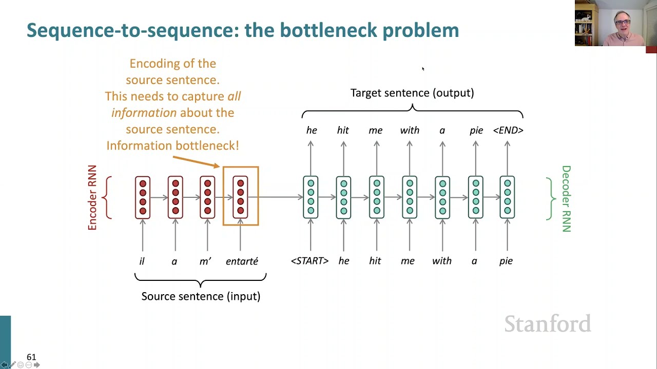
01:13:10.320 | So, we had this model of doing sequence to sequence models such as the neural machine translation. And the problem with this architecture is that we have this one hidden state, which has to encode all the information about the source sentence.

01:13:33.320 | So it acts as a kind of an information bottleneck. And that's all the information that the generation is conditioned on.

01:13:42.320 | Well, I didn't already mention one idea last time of how to get more information, where I said, look, maybe you could kind of average all of the vectors of the source to get a sentence representation.

01:13:55.320 | You know, that method turns out to be better for things like sentiment analysis and not so good for machine translation, where the order of words is very important to preserve.

01:14:07.320 | So it's, it seems like we would do better if somehow we could get more information from the source sentence while we're generating the translation.

01:14:20.320 | And in some sense, this just corresponds to what a human translator does, right? If you're a human translator, you read the sentence that you're meant to translate, and you maybe start translating a few words, but then you look back at the source sentence to see what else was in it and translate some more words.

01:14:38.320 | So very quickly after the first neural machine translation systems, people came up with the idea of maybe we could build a better neural MT model that did that.

01:14:50.320 | And that's the idea of attention.

01:14:54.320 | So the core idea is on each step of the decoder, we're going to use a direct link between the encoder and the decoder that will allow us to focus on a particular word or words in the source sequence and use it to help us generate what words come next.

01:15:19.320 | And I'll just go through now, showing you the pictures of what attention does. And then at the start of next time, we'll go through the equations in more detail.

01:15:32.320 | We generate, we use our encoder just as before and generate our representations, feed in our conditioning as before and say we're starting our translation.

01:15:45.320 | But at this point, we take this hidden representation and say, I'm going to use this hidden representation to look back at the source to get information directly from it.

01:15:58.320 | So what I will do is I will compare the hidden state of the decoder with the hidden state of the encoder at each position and generate an attention score, which is a kind of similarity score like a dot product.

01:16:18.320 | And then based on those attention scores, I'm going to calculate a probability distribution as to by using a softmax as usual to say which of these encoder states is most like my decoder state.

01:16:39.320 | And so we'll be training the model here to be saying, well, probably you should translate the first word of the sentence first. So that's where the attention should be placed.

01:16:49.320 | So then based on this attention distribution, which is a probability distribution coming out of the softmax, we're going to generate a new attention output.

01:17:04.320 | And so this attention output is going to be an average of the hidden states of the encoder model, but it's going to be a weighted average based on our attention distribution.

01:17:18.320 | And so we're then going to take that attention output, combine it with the hidden state of the decoder RNN, and together the two of them are then going to be used to predict via a softmax what word to generate first.

01:17:39.320 | And we hope to generate he.

01:17:42.320 | And then at that point, we sort of chug along and keep doing these same kind of computations at each position.

01:17:53.320 | There's a little side note here that says, sometimes we take the attention output from the previous step and also feed into the decoder along with the usual decoder input.

01:18:04.320 | So we're taking this attention output and actually feeding it back in to the hidden state calculation.

01:18:11.320 | And that can sometimes improve performance. And we actually have that trick in the assignment four system, and you can try it out.

01:18:20.320 | Okay, so we generate along and generate our whole sentence in this manner.

01:18:27.320 | And that's proven to be a very effective way of getting more information from the source sentence more flexibly to allow us to generate a good translation.

01:18:40.320 | I'll stop here for now. And at the start of next time, I'll finish this off by going through the actual equations for how attention works.

01:18:48.320 | Thanks for watching.

01:18:50.320 | [BLANK_AUDIO]

Stanford CS224N NLP with Deep Learning | Winter 2021 | Lecture 7 - Translation, Seq2Seq, Attention

Chapters