Lesson 12 (2019) - Advanced training techniques; ULMFiT from scratch

00:00:00.000 | Welcome to lesson 12.

00:00:04.080 | Wow, we're moving along.

00:00:06.560 | And this is an exciting lesson because it's where we're going to wrap up all the pieces

00:00:11.400 | both for computer vision and for NLP.

00:00:14.000 | And you might be surprised to hear that we're going to wrap up all the pieces for NLP because

00:00:17.760 | we haven't really done any NLP yet.

00:00:19.600 | But actually everything we've done is equally applicable to NLP.

00:00:24.560 | So there's very little to do to get a state-of-the-art result on IMDB sentiment analysis from scratch.

00:00:32.080 | So that's what we're going to do.

00:00:34.200 | Before we do, let's finally finish off this slide we've been going through for three lessons

00:00:38.960 | now.

00:00:39.960 | I promised, not promised, that we would get something state-of-the-art on ImageNet.

00:00:45.180 | Turns out we did.

00:00:46.180 | So you're going to see that today.

00:00:48.000 | So we're going to finish off, mix up, label smoothing, and resnets.

00:00:55.200 | Okay, so let's do it.

00:00:58.600 | Before we look at the new stuff, 09B learner.

00:01:06.840 | I've made a couple of minor changes that I thought you might be interested in.

00:01:11.240 | It's kind of like as you refactor things.

00:01:12.680 | So remember last week we refactored the learner to get rid of that awful separate runner.

00:01:17.280 | So there's just now one thing, made a lot of our code a lot easier.

00:01:20.280 | There's still this concept left behind that when you started fitting, you had to tell

00:01:25.320 | each callback what its learner or runner was.

00:01:28.400 | I've moved that, because they're all totally attached now, I've moved that to the init.

00:01:36.240 | And so now you can call add cbs to add a whole bunch of callbacks, or add cb to add one callback.

00:01:42.600 | And that happens automatically at the start of training.

00:01:45.220 | That's a very minor thing.

00:01:46.960 | More interesting was when I did this little reformatting exercise where I took all these

00:01:53.920 | callbacks that used to be on the line underneath the thing before them and lined them up over

00:01:58.360 | here and suddenly realized that now I can answer all the questions I have in my head

00:02:03.120 | about our callback system, which is what exactly are the steps in the training loop?

00:02:09.440 | What exactly are the callbacks that you can use in the training loop?

00:02:13.600 | Which step goes with which callback?

00:02:17.000 | Which steps don't have a callback?

00:02:18.760 | Are there any callbacks that don't have a step?

00:02:22.200 | So it's one of these interesting things where I really don't like the idea of automating

00:02:30.620 | your formatting and creating rules for formatting when something like this can just, as soon

00:02:35.240 | as I did this, I understood my code better.

00:02:38.560 | And for me, understanding my code is the only way to make it work.

00:02:41.840 | Because debugging machine learning code is awful.

00:02:45.920 | So you've got to make sure that the thing you write makes sense.

00:02:48.720 | It's got to be simple.

00:02:49.720 | It's got to be really simple.

00:02:50.720 | So this is really simple.

00:02:56.440 | Then more interestingly, we used to create the optimizer in init.

00:03:02.680 | And you could actually pass in an already created optimizer.

00:03:05.640 | I removed that.

00:03:06.960 | And the only thing now you can pass in is an optimization function.

00:03:10.040 | So something that will create an optimizer, which is what we've always been doing anyway.

00:03:14.060 | And by doing that, we can now create our optimizer when we start fitting.

00:03:19.120 | And that turns out to be really important.

00:03:21.560 | Because when we do things like discriminative learning rates and gradual unfreezing and

00:03:25.080 | layer groups and stuff, we can change things.

00:03:27.720 | And then when we fit, it will all just work.

00:03:30.440 | So that's a more significant -- it's like one line of code, but it's conceptually a

00:03:34.200 | very significant change.

00:03:36.040 | Okay. So that's some minor changes to 9B.

00:03:42.760 | And now let's move on to mixup and label smoothing.

00:03:46.720 | So I'm really excited about the stuff we saw at the end of the last lesson where we saw

00:03:52.120 | how we can use the GPU to do data augmentation.

00:03:55.440 | Fully randomized, fully GPU accelerated data augmentation using just plain PyTorch operations.

00:04:01.680 | I think that's a big win.

00:04:04.560 | But it's quite possible we don't need that kind of data augmentation anymore.

00:04:10.680 | Because in our experimentation with this data augmentation called mixup, we found we can

00:04:15.600 | remove most other data augmentation and get amazingly good results.

00:04:20.960 | So it's just a kind of a simplicity result.

00:04:23.760 | And also when you use mixup, you can train for a really long time and get really good

00:04:27.760 | results.

00:04:29.200 | So let me show you mixup.

00:04:31.040 | And in terms of the results, you can get -- what happened in the bag of tricks paper was they

00:04:38.920 | -- when they turned mixup on, they also started training for 200 epochs instead of 120.

00:04:48.480 | So be a bit careful when you interpret their paper table when it goes from label smoothing

00:04:56.520 | 94.1 to mixup without distillation 94.6.

00:05:04.200 | They're also nearly doubling the number of epochs they do.

00:05:07.120 | But you can kind of get a sense that you can get big decrease in error.

00:05:12.640 | The other thing they mention in the paper is distillation.

00:05:15.120 | I'm not going to talk about that because it's a thing where you pre-train some much bigger

00:05:19.880 | model like a ResNet-152, and then you try and train something that predicts the output

00:05:23.960 | of that.

00:05:24.960 | The idea of training a really big model, to train a smaller model, it's interesting, but

00:05:29.560 | it's not exactly training in the way I normally think about it.

00:05:32.440 | So we're not looking at distillation.

00:05:33.800 | It would be an interesting assignment if somebody wanted to try adding it to the notebooks though.

00:05:39.680 | You have all the information and I think all the skills you need to do that now.

00:05:43.280 | All right.

00:05:45.740 | So mixup, we start by grabbing our ImageNet data set and we grab the MakeRGB and resize

00:05:55.960 | and turn it into a float tensor.

00:05:58.360 | This is just our quick and dirty resize, we're already doing this for testing purposes.

00:06:02.000 | Split it up, create a data bunch, all the normal stuff.

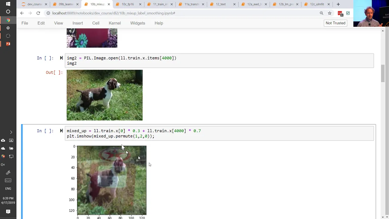
00:06:07.060 | But what we're going to do is we're going to take an image like this and an image like

00:06:15.080 | this and we're going to combine them.

00:06:19.560 | We're going to take 0.3 times this image plus 0.7 times this image and this is what it's

00:06:27.840 | going to look like.

00:06:29.620 | Unfortunately, Silva and I have different orderings of file names on our thing, so I wrote, it's

00:06:35.200 | a French horn and a tench but actually Silva clearly doesn't have French horn or tenches

00:06:39.200 | but you get the idea.

00:06:40.520 | It's a mixup of two different images.

00:06:42.880 | So we're going to create a greater augmentation where every time we predict something we're

00:06:49.200 | going to be predicting a mix of two things like this.

00:06:52.160 | So we're going to both take the linear combination, 0.3 and 0.7, of the two images but then we're

00:07:01.080 | going to have to do that for the labels as well, right?

00:07:03.520 | There's no point predicting the one hot encoded output of this breed of doggy where there's

00:07:11.500 | also a bit of a gas pump.

00:07:14.000 | So we're also going to have, we're not going to have one hot encoded output, we're going

00:07:17.560 | to have a 0.7 encoded doggy and a 0.3 encoded gas pump.

00:07:24.480 | So that's the basic idea.

00:07:28.340 | So the mixup paper was super cool.

00:07:34.060 | Wow, there are people talking about things that aren't deep learning.

00:07:40.720 | I guess that's their priorities.

00:07:46.640 | So the paper's a pretty nice, easy read by paper standards and I would definitely suggest

00:07:52.340 | you check it out.

00:07:57.560 | So I've told you what we're going to do, implementation-wise, we have to decide what number to use here.

00:08:03.360 | Is it 0.3 or 0.1 or 0.5 or what?

00:08:06.600 | And this is a data augmentation method, so the answer is we'll randomize it.

00:08:10.560 | But we're not going to randomize it from 0 to 1 uniform or 0 to 0.5 uniform, but instead

00:08:16.960 | we're going to randomize it using shapes like this.

00:08:22.240 | In other words, when we grab a random number, most of the time it'll be really close to

00:08:27.760 | 0 or really close to 1, and just occasionally it'll be close to 0.5.

00:08:31.680 | So that way most of the time it'll be pretty easy for our model because it'll be predicting

00:08:35.960 | one and only one thing, and just occasionally it'll be predicting something that's a pretty

00:08:41.080 | evenly mixed combination.

00:08:43.360 | So the ability to grab random numbers, that this is basically the histogram, the smoothed

00:08:50.120 | histogram of how often we're going to see those numbers, is called sampling from a probability

00:08:57.880 | distribution.

00:08:58.880 | And basically in nearly all these cases you can start with a uniform random number or

00:09:03.320 | a normal random number and put it through some kind of function or process to turn it

00:09:07.780 | into something like this.

00:09:08.780 | So the details don't matter at all.

00:09:13.240 | But the paper points out that this particular shape is nicely characterized by something

00:09:17.240 | called the beta distribution, so that's what we're going to use.

00:09:21.360 | So it was interesting drawing these because it requires a few interesting bits of math,

00:09:29.800 | which some of you may be less comfortable with or entirely uncomfortable with.

00:09:35.480 | For me, every time I see this function, which is called the gamma function, I kind of break

00:09:42.480 | out in sweats, not just because I've got a cold, but it's like the idea of functions

00:09:47.240 | that I don't-- like how do you describe this thing?

00:09:50.400 | But actually, it turns out that like most things, once you look at it, it's actually

00:09:56.080 | pretty straightforward.

00:09:57.080 | And we're going to be using this function, so I'll just quickly explain what's going

00:09:59.520 | on.

00:10:00.520 | We're going to start with a factorial function, so 1 times 2 times 3 times 4, whatever, right?

00:10:06.960 | And here these red dots is just the value of the factorial function for a few different

00:10:11.720 | places.

00:10:14.720 | But don't think of the factorial function as being 1 times 2 times 3 times 4, or times

00:10:20.360 | n, whatever, but divide both sides by n, and now you've got-- or divide both sides by n,

00:10:28.720 | and now you've got like factorial n divided by n equals 1 times 2 times 3, so it equals

00:10:37.120 | the factorial of n minus 1.

00:10:39.960 | And so when you define it like that, you suddenly realize there's no reason that you kind of

00:10:43.440 | have a function that's not just on the integers-- not just on the integers, but is everywhere.

00:10:49.120 | This is the point where I stop with the math, right?

00:10:51.000 | Because to me, if I need a sine function, or a log function, or an x-punk fin, or whatever,

00:10:55.040 | I type it into my computer and I get it, right?

00:10:57.140 | So the actual how you get it is not at all important.

00:11:00.480 | But the fact of knowing what these functions are and how they're defined is useful.

00:11:05.680 | PyTorch doesn't have this function.

00:11:07.640 | Weirdly enough, they have a log gamma function.

00:11:09.760 | So we can take log gamma and go e to the power of that to get a gamma function.

00:11:13.480 | And you'll see here, I am breaking my no Greek letters rule.

00:11:17.880 | And the reason I'm breaking that rule is because a function like this doesn't have a kind of

00:11:24.200 | domain-specific meaning, or a pure physical analogy, which is how we always think about

00:11:30.360 | it.

00:11:31.360 | It's just a math function.

00:11:32.560 | And so we call it gamma, right?

00:11:34.480 | And so if you're going to call it gamma, you may as well write it like that.

00:11:38.280 | And why this matters is when you start using it.

00:11:42.400 | Like look at the difference between writing it out with the actual Unicode and operators

00:11:49.280 | versus what would happen if you wrote it out long form in Python.

00:11:54.400 | Like when you're comparing something to a paper, you want something that you can look

00:11:57.920 | at and straight away say like, oh, that looks very familiar.

00:12:02.080 | And as long as it's not familiar, you might want to think about how to make it more familiar.

00:12:06.160 | So I just briefly mentioned that writing these math symbols nowadays is actually pretty easy.

00:12:12.480 | On Linux, there's a thing called a compose key which is probably already set up for you.

00:12:16.880 | And if you Google it, you can learn how to turn it on.

00:12:18.800 | And it's basically like you'll press like the right alt button or the caps lock button.

00:12:22.400 | You can choose what your compose key is.

00:12:24.360 | And then a few more letters.

00:12:26.080 | So for example, all the Greek letters are compose and then star, and then the English

00:12:30.000 | letter that corresponds with it.

00:12:31.560 | So for example, if I want to do lambda, I would go composed L. So it's just as quick

00:12:38.200 | as typing non Unicode characters.

00:12:40.920 | Most of the Greek letters are available on a Mac keyboard just with option.

00:12:43.760 | Unfortunately, nobody's created a decent compose key for Mac yet.

00:12:46.960 | There's a great compose key for Windows called win compose.

00:12:49.920 | Anybody who's working with, you know, Greek letters should definitely install and learn

00:12:55.120 | to use these things.

00:12:58.360 | So there's our gamma function nice and concise.

00:13:01.520 | It looks exactly like the paper.

00:13:03.320 | And so it turns out that this is how you calculate the value of the beta function, which is the

00:13:07.080 | beta distribution.

00:13:08.160 | And so now here it is.

00:13:09.160 | So as I said, the details aren't important, but they're the tools that you can use.

00:13:13.120 | The basic idea is that we now have something where we can pick some parameter, which is

00:13:17.720 | called alpha, where if it's high, then it's much more likely that we get a equal mix.

00:13:25.040 | And if it's low, it's very unlikely.

00:13:27.200 | And this is really important because for data augmentation, we need to be able to tune a

00:13:30.240 | lever that says how much regularization am I doing?

00:13:34.040 | How much augmentation am I doing?

00:13:35.400 | So you can move your alpha up and down.

00:13:37.920 | And the reason it's important to be able to print these plots out is that when you change

00:13:41.560 | your alpha, you want to plot it out and see what it looks like, right?

00:13:45.000 | Make sure it looks sensible, okay?

00:13:49.600 | So it turns out that all we need to do then is we don't actually have to 0.7 hot encode

00:13:59.640 | one thing and 0.3 hot encode another thing.

00:14:02.360 | It's actually identical to simply go, I guess it is lambda times the first loss plus 1 minus

00:14:11.760 | lambda times the second loss.

00:14:12.920 | I guess we're using t here.

00:14:15.200 | So that's actually all we need to do.

00:14:18.160 | So this is our mixup.

00:14:23.160 | And again, as you can see, we're using the same letters that we'd expect to see in the

00:14:25.920 | paper.

00:14:26.920 | So everything should look very familiar.

00:14:28.720 | And mixup, remember, is something which is going to change our loss function.

00:14:33.400 | So we need to know what loss function to change.

00:14:35.680 | So when you begin fitting, you find out what the old loss function on the learner was when

00:14:42.200 | you store it away.

00:14:43.720 | And then when we calculate loss, we can just go ahead and say, oh, if it's invalidation,

00:14:49.680 | there's no mixup involved.

00:14:51.300 | And if we're training, then we'll calculate the loss on two different sets of images.

00:14:57.400 | One is just the regular set, and the second is we'll grab all the other images and randomly

00:15:04.120 | permute one and randomly pick one to share with.

00:15:08.720 | So we do that for the image, and we do that for the loss.

00:15:13.940 | And that's basically it.

00:15:17.480 | Couple of minor things to mention.

00:15:19.160 | In the last lesson, I created an EWMA function, Exponentially Weighted Moving Average Function,

00:15:25.880 | which is a really dumb name for it, because actually it was just a linear combination

00:15:30.000 | of two things.

00:15:31.000 | It was like V times alpha plus V1 times alpha plus V2 times 1 minus alpha.

00:15:38.280 | You create exponentially weighted moving averages with it by applying it multiple times, but

00:15:42.600 | the actual function is a linear combination, so I've renamed that to linear combination,

00:15:46.880 | and you'll see that so many places.

00:15:48.240 | So this mixup is a linear combination of our actual images and some randomly permuted images

00:15:55.440 | in that mini-batch.

00:15:57.640 | And our loss is a linear combination of the loss of our two different parts, our normal

00:16:04.320 | mini-batch and our randomly permuted mini-batch.

00:16:06.800 | One of the nice things about this is if you think about it, this is all being applied

00:16:09.840 | on the GPU.

00:16:11.380 | So this is pretty much instant.

00:16:14.160 | So super powerful augmentation system, which isn't going to add any overhead to our code.

00:16:22.480 | One thing to be careful of is that we're actually replacing the loss function, and loss functions

00:16:30.960 | have something called a reduction.

00:16:34.280 | And most PyTorch loss functions, you can say, after calculating the loss function for everything

00:16:39.400 | in the mini-batch, either return a rank 1 tensor of all of the loss functions for the

00:16:44.880 | mini-batch, or add them all up, or take the average.

00:16:49.200 | We pretty much always take the average.

00:16:50.200 | But we just have to make sure that we do the right thing.

00:16:53.800 | So I've just got a little function here that does the mean or sum, or nothing at all, as

00:16:58.400 | requested.

00:16:59.960 | And so then we need to make sure that we create our new loss function, that at the end, it's

00:17:07.240 | going to reduce it in the way that they actually asked for.

00:17:11.400 | But then we have to turn off the reduction when we actually do mixup, because we actually

00:17:16.640 | need to calculate the loss on every image for both halves of our mixup.

00:17:23.280 | So this is a good place to use a context manager, which we've seen before.

00:17:27.640 | So we just created a tiny little context manager, which will just find out what the previous

00:17:32.020 | reduction was, save it away, get rid of it, and then put it back when it's finished.

00:17:38.420 | So there's a lot of minor details there.

00:17:41.280 | But with that in place, the actual mixup itself is very little code.

00:17:44.600 | It's a single callback.

00:17:46.320 | And we can then run it in the usual way.

00:17:49.440 | Just add mixup.

00:17:52.440 | Our default alpha here is 0.4.

00:17:55.560 | And I've been mainly playing with alpha at 0.2, so this is a bit more than I'm used to.

00:17:59.380 | But somewhere around that vicinity is pretty normal.

00:18:04.500 | So that's mixup.

00:18:05.660 | And that's like-- it's really interesting, because you could use this for layers other

00:18:13.320 | than the input layer.

00:18:15.020 | You could use it on the first layer, maybe with the embeddings.

00:18:18.040 | So you could do mixup augmentation in NLP, for instance.

00:18:23.920 | That's something which people haven't really dug into deeply yet.

00:18:28.000 | But it seems to be an opportunity to add augmentation in many places where we don't really see it

00:18:34.880 | at the moment.

00:18:35.880 | Which means we can train better models with less data, which is why we're here.

00:18:41.680 | So here's a problem.

00:18:42.760 | How does Softmax interact with this?

00:18:45.440 | So now we've drawn some random number lambda.

00:18:49.120 | It's 0.7.

00:18:50.120 | So I've got 0.7 of a dog and 0.3 of a gas station.

00:18:53.640 | And the correct answer would be a rank one tensor which has 0.7 in one spot and 0.3 in

00:19:01.520 | the other spot and 0 everywhere else.

00:19:04.840 | Softmax isn't going to want to do that for me, because Softmax really wants just one

00:19:08.400 | of my values to be high, because it's got an e to the top, as we've talked about.

00:19:14.860 | So we-- to really use mixup well-- and not just use mixup well, but any time your data

00:19:21.560 | is-- the labels on the data, you're not 100% sure they're correct.

00:19:25.720 | You don't want to be asking your model to predict one.

00:19:30.320 | You want to be-- don't predict, I'm 100% sure it's this label, because you've got label

00:19:35.040 | noise.

00:19:36.040 | You've got incorrect labels, or you've got mixup, mixing, or whatever.

00:19:38.960 | So instead, we say, oh, don't use one hot encoding for the dependent variable, but use a little

00:19:45.880 | bit less than one hot encoding.

00:19:47.640 | So say 0.9 hot encoding.

00:19:50.000 | So then the correct answer is to say, I'm 90% sure this is the answer.

00:19:54.720 | And then all of your probabilities have to add to one.

00:19:57.360 | So then all of the negatives, you just put 0.1 divided by n minus one, and all the rest.

00:20:03.080 | And that's called label smoothing.

00:20:05.640 | And it's a really simple but astonishingly effective way to handle noisy labels.

00:20:13.600 | I keep on hearing people saying, oh, we can't use deep learning in this medical problem,

00:20:20.560 | because the diagnostic labels in the reports are not perfect, and we don't have a gold

00:20:24.980 | standard and whatever.

00:20:26.980 | It actually turns out that particularly if you lose label smoothing, noisy data is generally

00:20:31.400 | not an option.

00:20:32.400 | Like, there's plenty of examples of people using this where they literally randomly permute

00:20:38.440 | half the labels to make them like 50% wrong, and they still get good results, really good

00:20:42.680 | results.

00:20:44.160 | So don't listen to people in your organization saying, we can't start modeling until we do

00:20:50.880 | all this cleanup work.

00:20:52.900 | Start modeling right now.

00:20:53.900 | See if the results are OK.

00:20:56.200 | And if they are, then maybe you can skip all the cleanup work or do them simultaneously.

00:21:01.360 | So label smoothing ends up just being the cross entropy loss as before times if epsilon

00:21:09.960 | is 0.1 and 0.9 plus 0.1 times the cross entropy for everything divided by n.

00:21:17.800 | And the nice thing is that's another linear combination.

00:21:21.040 | So once you kind of create one of these little mathematical refactorings that tend to pop

00:21:24.520 | up everywhere and make your code a little bit easier to read and a little bit harder

00:21:28.760 | to stuff up, every time I have to write a piece of code, there's a very high probability

00:21:33.520 | that I'm going to screw it up.

00:21:34.860 | So the less I have to write, the less debugging I'm going to have to do later.

00:21:39.540 | So we can just pop that in as a loss function and away we go.

00:21:46.400 | So that's a super powerful technique which has been around for a couple of years, those

00:21:53.400 | two techniques, but not nearly as widely used as they should be.

00:21:58.840 | Then if you're using a Volta, Tensor Core, 2080, any kind of pretty much any current

00:22:06.120 | generation Nvidia graphics card, you can train using half precision floating point in theory

00:22:13.680 | like 10 times faster.

00:22:16.040 | In practice it doesn't quite work out that way because there's other things going on,

00:22:18.920 | but we certainly often see 3x speedups.

00:22:22.880 | So the other thing we've got is some work here to allow you to train in half precision

00:22:28.600 | floating point.

00:22:30.560 | Now the reason it's not as simple as saying model.half, which would convert all of your

00:22:35.080 | weights and biases and everything to half precision floating point, is because of this.

00:22:41.200 | This is from Nvidia's materials and what they point out is that you can't just use half

00:22:48.840 | precision everywhere because it's not accurate, it's bumpy.

00:22:53.800 | So it's hard to get good useful gradients if you do everything in half precision, particularly

00:22:59.680 | often things will round off to zero.

00:23:02.300 | So instead what we do is we do the forward pass in FP16, we do the backward pass in FP16,

00:23:09.980 | so all the hard work is done in half precision floating point, and pretty much everywhere

00:23:14.800 | else we convert things to full precision floating point and do everything else in full precision.

00:23:20.680 | So for example, when we actually apply the gradients by multiplying the value of the learning

00:23:23.800 | rate, we do that in FP32, single precision.

00:23:28.780 | And that means that if your learning rate's really small, in FP16 it might basically round

00:23:34.960 | down to zero, so we do it in FP32.

00:23:40.280 | In FastAI version one, we wrote all this by hand.

00:23:44.720 | For the lessons, we're experimenting with using a library from Nvidia called Apex.

00:23:50.120 | Apex basically have some of the functions to do this there for you.

00:23:55.520 | So we're using it here, and basically you can see there's a thing called model to half

00:24:01.380 | where we just go model to half, batch norm, goes to float, and so forth.

00:24:05.700 | So these are not particularly interesting, but they're just going through each one and

00:24:09.480 | making sure that the right layers have the right types.

00:24:13.160 | So once we've got those kind of utility functions in place, the actual callback's really quite

00:24:20.120 | small and you'll be able to map every stage to that picture I showed you before.

00:24:26.520 | So you'll be able to see when we start fitting, we convert the network to half-precision floating

00:24:31.640 | point, for example.

00:24:33.240 | One of the things that's kind of interesting is there's something here called loss scale.

00:24:38.920 | After the backward pass, well probably more interestingly, after the loss is calculated,

00:24:48.080 | we multiply it by this number called loss scale, which is generally something around

00:24:51.480 | 512.

00:24:52.640 | The reason we do that is that losses tend to be pretty small in a region where half-precision

00:24:57.880 | floating point's not very accurate.

00:24:59.720 | So we just multiply it by 512, put it in a region that is accurate.

00:25:03.360 | And then later on, in the backward step, we just divide by that again.

00:25:06.600 | So that's a little tweak, but it's the difference we find generally between things working and

00:25:11.280 | not working.

00:25:12.840 | So the nice thing is now, we have something which you can just add mixed precision and

00:25:20.360 | train and you will get often 2x, 3x speed up, certainly on vision models, also on transformers,

00:25:32.200 | quite a few places.

00:25:34.440 | One obvious question is, is 512 the right number?

00:25:39.480 | And it turns out getting this number right actually does make quite a difference to your

00:25:42.560 | training.

00:25:43.720 | And so something slightly more recently is called dynamic loss scaling, which literally

00:25:48.200 | tries a few different values of loss scale to find out at what point does it become infinity.

00:25:54.040 | And so it dynamically figures out the highest loss scale we can go to.

00:25:59.160 | And so this version just has the dynamic loss scaling added.

00:26:03.680 | It's interesting that sometimes training with half-precision gives you better results than

00:26:08.800 | training with FP32 because there's just, I don't know, a bit more randomness.

00:26:13.120 | Maybe it regularizes a little bit, but generally it's super, super similar, just faster.

00:26:18.280 | We have a question about mixup.

00:26:20.160 | Great.

00:26:21.560 | Is there an intuitive way to understand why mixup is better than other data augmentation

00:26:26.120 | techniques?

00:26:30.600 | I think one of the things that's really nice about mixup is that it doesn't require any

00:26:36.160 | domain-specific thinking.

00:26:38.360 | Do we flip horizontally or also vertically?

00:26:40.840 | How much can we rotate?

00:26:43.440 | It doesn't create any kind of lossiness, like in the corners, there's no reflection padding

00:26:47.160 | or black padding.

00:26:48.160 | So it's kind of quite nice and clean.

00:26:52.800 | It's also almost infinite in terms of the number of different images it can create.

00:26:59.240 | So you've kind of got this permutation of every image with every other image, which

00:27:04.040 | is already giant, and then in different mixes.

00:27:06.800 | So it's just a lot of augmentation that you can do with it.

00:27:13.920 | And there are other similar things.

00:27:16.600 | So there's another thing which, there's something called cutout where you just delete a square

00:27:22.240 | and replace it with black.

00:27:23.680 | There's another one where you delete a square and replace it with random pixels.

00:27:27.200 | Something I haven't seen, but I'd really like to see people do, is to delete a square and

00:27:30.640 | replace it with a different image.

00:27:32.120 | So I'd love somebody to try doing mix-up, but instead of taking the linear combination,

00:27:38.080 | instead pick an alpha-sized, sorry, a lambda percent of the pixels, like in a square, and

00:27:45.280 | paste them on top.

00:27:47.320 | There's another one which basically finds four different images and puts them in four

00:27:52.000 | corners.

00:27:53.000 | So there's a few different variations.

00:27:55.280 | And they really get great results, and I'm surprised how few people are using them.

00:28:02.440 | So let's put it all together.

00:28:04.320 | So here's emotionet.

00:28:06.720 | So let's use our random resize crop, a minimum scale of 0.35 we find works pretty well.

00:28:15.240 | And we're not going to do any other, other than flip, we're not going to do any other

00:28:18.760 | augmentation.

00:28:21.320 | And now we need to create a model.

00:28:25.000 | So far, all of our models have been boring convolutional models.

00:28:30.760 | But obviously what we really want to be using is a resnet model.

00:28:36.000 | We have the xresnet, which there's some debate about whether this is the mutant version of

00:28:41.320 | resnet or the extended version of resnet.

00:28:44.300 | So you can choose what the x stands for.

00:28:47.840 | And basically the xresnet is the bag of tricks, is basically the bag of tricks resnet.

00:28:58.780 | So they have a few suggested tweaks to resnet.

00:29:07.240 | And here they are.

00:29:09.520 | So these are their little tweaks.

00:29:13.200 | So the first tweak is something that we've kind of talked about, and they call it resnet

00:29:17.360 | c.

00:29:18.360 | And it's basically, hey, let's not do a big seven by seven convolution as our first layer,

00:29:24.280 | because that's super inefficient.

00:29:26.920 | And it's just a single linear model, which doesn't have much kind of richness to it.

00:29:33.180 | So instead, let's do three comms in a row, three by three, right?

00:29:38.940 | And so three, three by three comms in a row, if you think about it, the receptive field

00:29:43.040 | of that final one is still going to be about seven by seven, right?

00:29:48.160 | But it's got there through a much richer set of things that it can learn, because it's

00:29:52.560 | a three layer neural net.

00:29:54.920 | So that's the first thing that we do in our xresnet.

00:29:59.600 | So here is xresnet.

00:30:03.840 | And when we create it, we set up how many filters are they going to be for each of the

00:30:09.240 | first three layers?

00:30:10.240 | So the first three layers will start with channels in, inputs.

00:30:14.280 | So that'll default to three, because normally we have three channel images, right?

00:30:18.280 | And the number of outputs that we'll use for the first layer will be that plus one times

00:30:22.740 | eight.

00:30:24.440 | Why is that?

00:30:25.640 | It's a bit of a long story.

00:30:27.700 | One reason is that that gives you 32 at the second layer, which is the same as what the

00:30:34.840 | bag of tricks paper recommends.

00:30:41.400 | As you can see.

00:30:42.840 | The second reason is that I've kind of played around with this quite a lot to try to figure

00:30:50.120 | out what makes sense in terms of the receptive field, and I think this gives you the right

00:30:55.360 | amount.

00:30:56.360 | Sometimes eight is here because video graphics cards like everything to be a multiple of

00:31:04.560 | eight.

00:31:05.560 | So if this is not eight, it's probably going to be slower.

00:31:07.300 | But one of the things here is now if you have like a one channel input, like black and white,

00:31:12.900 | or a five channel input, like some kind of hyperspectral imaging or microscopy, then

00:31:17.600 | you're actually changing your model dynamically to say, oh, if I've got more inputs, then

00:31:22.680 | my first layer should have more activations.

00:31:24.640 | Which is not something I've seen anybody do before, but it's a kind of really simple,

00:31:29.000 | nice way to improve your ResNet for different kinds of domains.

00:31:33.880 | So that's the number of filters we have for each layer.

00:31:37.360 | So our stem, so the stem is the very start of a CNN.

00:31:41.620 | So our stem is just those three conflayers.

00:31:46.160 | So that's all the paper says.

00:31:49.040 | What's a conflayer?

00:31:50.840 | A conflayer is a sequential containing a bunch of layers, which starts with a conf of some

00:31:58.520 | stride, followed by a batch norm, and then optionally followed by an activation function.

00:32:05.920 | And our activation function, we're just going to use ReLU for now, because that's what they're

00:32:08.520 | using in the paper.

00:32:11.200 | The batch norm, we do something interesting.

00:32:13.980 | This is another tweak from the bag of tricks, although it goes back a couple more years

00:32:17.160 | than that.

00:32:18.420 | We initialize the batch norm, sometimes to have weights of 1, and sometimes to have weights

00:32:27.840 | of 0.

00:32:30.320 | Why do we do that?

00:32:32.000 | Well, all right.

00:32:34.960 | Have a look here at ResNet D. This is a standard ResNet block.

00:32:41.480 | This path here normally doesn't have the conv and the average pool.

00:32:45.120 | So pretend they're not there.

00:32:46.120 | We'll talk about why they're there sometimes in a moment.

00:32:48.080 | But then this is just the identity.

00:32:50.320 | And the other goes 1 by 1 conv, 3 by 3 conv, 1 by 1 conv.

00:32:55.920 | And remember, in each case, it's conv batch norm ReLU, conv batch norm ReLU.

00:32:59.720 | And then what actually happens is it then goes conv batch norm, and then the ReLU happens

00:33:03.720 | after the plus.

00:33:05.600 | There's another variant where the ReLU happens before the plus, which is called preact or

00:33:09.920 | preactivation ResNet.

00:33:10.920 | Turns out it doesn't work quite as well for smaller models, so we're using the non-preact

00:33:16.520 | version.

00:33:17.520 | Now, see this conv here?

00:33:20.920 | What if we set the batch norm layer weights there to 0?

00:33:25.280 | What's going to happen?

00:33:26.280 | Well, we've got an input.

00:33:27.700 | This is identity.

00:33:29.040 | This does some conv, some conv, some conv, and then batch norm where the weights are

00:33:33.560 | 0, so everything gets multiplied by 0.

00:33:35.800 | And so out of here comes 0.

00:33:39.280 | So why is that interesting?

00:33:40.480 | Because now we're adding 0 to the identity block.

00:33:43.800 | So in other words, the whole block does nothing at all.

00:33:47.840 | That's a great way to initialize a model, right?

00:33:50.560 | Because we really don't want to be in a position, as we've seen, where if you've got a thousand

00:33:54.200 | layers deep model, that any layer is even slightly changing the variance because they

00:33:59.160 | kind of cause the gradients to spiral off to 0 or to infinity.

00:34:03.320 | This way, literally, the entire activations are the same all the way through.

00:34:09.240 | So that's what we do.

00:34:10.640 | We set the 1, 2, 3 third conv layer to have 0 in that batch norm layer.

00:34:21.760 | And this lets us train very deep models at very high learning rates.

00:34:26.240 | You'll see nearly all of the academic literature about this talks about large batch sizes because,

00:34:30.800 | of course, academics, particularly at big companies like Google and OpenAI and Nvidia

00:34:35.360 | and Facebook, love to show off their giant data centers.

00:34:39.760 | And so they like to say, oh, if we do 1,000 TPUs, how big a batch size can we create?

00:34:45.040 | But for us normal people, these are also interesting because the exact same things tell us how

00:34:50.000 | high a learning rate can we go, right?

00:34:52.220 | So the exact same things that let you create really big batch sizes, so you do a giant

00:34:55.320 | batch and then you take a giant step, well, we can just take a normal sized batch, but

00:35:00.680 | a much bigger than usual step.

00:35:02.600 | And by using higher learning rates, we train faster and we generalize better.

00:35:07.400 | And so that's all good.

00:35:08.400 | So this is a really good little trick.

00:35:10.840 | Okay.

00:35:13.040 | So that's conv layer.

00:35:17.680 | So there's our stem.

00:35:20.040 | And then we're going to create a bunch of res blocks.

00:35:24.160 | So a res block is one of these, except this is an identity path, right?

00:35:30.640 | Unless we're doing a res net 34 or a res net 18, in which case one of these comms goes

00:35:38.840 | away.

00:35:39.840 | So res net 34 and res net 18 only have two cons here and res net 50 onwards have three

00:35:45.400 | cons here.

00:35:47.120 | So and then in res net 50 and above, the second conv, they actually squish the number of channels

00:35:54.200 | down by four and then they expand it back up again.

00:35:57.760 | So it could go like 64 channels to 16 channels to 64 channels.

00:36:02.600 | Let's call it a bottleneck layer.

00:36:04.560 | So a bottleneck block is the normal block for larger res nets.

00:36:08.420 | And then just two three by three comms is the normal for smaller res nets.

00:36:14.200 | So you can see in our res block that we pass in this thing called expansion.

00:36:19.360 | It's either one or four.

00:36:20.860 | It's one if it's res net 18 or 34, and it's four if it's bigger, right?

00:36:26.240 | And so if it's four, well, if it's expansion equals one, then we just add one extra conv,

00:36:31.960 | right?

00:36:32.960 | Oh, sorry.

00:36:33.960 | The first conv is always a one by one, and then we add a three by three conv, or if expansion

00:36:38.600 | equals four, we add two extra comms.

00:36:42.680 | So that's what the res blocks are.

00:36:46.440 | Now I mentioned that there's two other things here.

00:36:50.600 | Why are there two other things here?

00:36:52.960 | Well, we can't use standard res blocks all the way through our model, can we?

00:36:58.120 | Because a res block can't change the grid size.

00:37:01.120 | We can't have a stride two anywhere here, because if we had a stride two somewhere here,

00:37:07.260 | we can't add it back to the identity because they're now different sizes.

00:37:11.120 | Also we can't change the number of channels, right?

00:37:14.260 | Because if we change the number of channels, we can't add it to the identity.

00:37:17.440 | So what do we do?

00:37:18.680 | Well, as you know, from time to time, we do like to throw in a stride two, and generally

00:37:23.840 | when we throw in a stride two, we like to double the number of channels.

00:37:27.520 | And so when we do that, we're going to add to the identity path two extra layers.

00:37:32.520 | We'll add an average pooling layer, so that's going to cause the grid size to shift down

00:37:37.200 | by two in each dimension, and we'll add a one by one conv to change the number of filters.

00:37:43.300 | So that's what this is.

00:37:45.060 | And this particular way of doing it is specific to the x res net, and it gives you a nice

00:37:51.360 | little boost over the standard approach, and so you can see that here.

00:37:58.600 | If the number of inputs is different to the number of filters, then we add an extra conv

00:38:02.800 | layer, otherwise we just do no op, no operation, which is defined here.

00:38:10.480 | And if the stride is something other than one, we add an average pooling, otherwise it's

00:38:15.160 | a no op, and so here is our final res net block calculation.

00:38:20.580 | So that's the res block.

00:38:23.680 | So tweak for res net d is this way of doing the, they call it a downsampling path.

00:38:32.840 | And then the final tweak is the actual ordering here of where the stride two is.

00:38:37.400 | Usually the stride two in normal res net is at the start, and then there's a three by

00:38:42.880 | three after that.

00:38:44.200 | Doing a stride two on a one by one conv is a terrible idea, because you're literally

00:38:48.400 | throwing away three quarters of the data, and it's interesting, it took people years

00:38:53.240 | to realize they're literally throwing away three quarters of the data, so the bag of

00:38:57.080 | tricks folks said, let's just move the stride two to the three by three, and that makes

00:39:01.160 | a lot more sense, right?

00:39:02.160 | Because a stride two, three by three, you're actually hitting every pixel.

00:39:07.480 | So the reason I'm mentioning these details is so that you can read that paper and spend

00:39:12.760 | time thinking about each of those res net tweaks, do you understand why they did that?

00:39:18.280 | Right?

00:39:19.280 | It wasn't some neural architecture search, try everything, brainless, use all our computers

00:39:25.800 | approach.

00:39:26.800 | So let's sit back and think about how do we actually use all the inputs we have, and how

00:39:33.040 | do we actually take advantage of all the computation that we're doing, right?

00:39:37.600 | So it's a very, most of the tweaks are stuff that exists from before, and they've cited

00:39:43.220 | all those, but if you put them all together, it's just a nice, like, here's how to think

00:39:47.000 | through architecture design.

00:39:52.400 | And that's about it, right?

00:39:53.640 | So we create a res net block for every res layer, and so here it is, creating the res

00:40:02.080 | net block, and so now we can create all of our res nets by simply saying, this is how

00:40:09.320 | many blocks we have in each layer, right?

00:40:12.560 | So res net 18 is just two, two, two, two, 34 is three, four, six, three, and then secondly

00:40:17.560 | is changing the expansion factor, which as I said for 18 and 34 is one, and for the bigger

00:40:23.520 | ones is four.

00:40:26.200 | So that's a lot of information there, and if you haven't spent time thinking about architecture

00:40:30.440 | before, it might take you a few reads and lessons to put the sink in, but I think it's

00:40:35.120 | a really good idea to try to spend time thinking about that, and also to, like, experiment,

00:40:41.000 | right?

00:40:42.000 | And try to think about what's going on.

00:40:44.580 | The other thing to point out here is that this -- the way I've written this, it's like

00:40:53.000 | this is the whole -- this is the whole res net, right, other than the definition of conflayer,

00:40:59.200 | this is the whole res net.

00:41:00.320 | It fits on the screen, and this is really unusual.

00:41:03.720 | Most res nets you see, even without the bag of tricks, 500, 600, 700 lines of code, right?

00:41:10.720 | And if every single line of code has a different arbitrary number at 16 here and 32 there and

00:41:17.480 | average pool here and something else there, like, how are you going to get it right?

00:41:20.800 | And how are you going to be able to look at it and say, what if I did this a little bit

00:41:24.280 | differently?

00:41:26.240 | So for research and for production, you want to get your code refactored like this for

00:41:32.880 | your architecture so that you can look at it and say, what exactly is going on, is it

00:41:37.960 | written correctly, okay, I want to change this to be in a different layer, how do I

00:41:42.680 | do it?

00:41:45.000 | It's really important for effective practitioners to be able to write nice, concise architectures

00:41:52.440 | so that you can change them and understand them.

00:41:55.520 | Okay.

00:41:57.000 | So that's our X res net.

00:41:58.960 | We can train it with or without mixup, it's up to us.

00:42:03.520 | Label smoothing cross entropy is probably always a good idea, unless you know that your labels

00:42:07.480 | are basically perfect.

00:42:08.480 | Let's just create a little res net 18.

00:42:13.320 | And let's check out to see what our model is doing.

00:42:16.800 | So we've already got a model summary, but we're just going to rewrite it to use our,

00:42:20.680 | the new version of learner that doesn't have runner anymore.

00:42:23.940 | And so we can print out and see what happens to our shapes as they go through the model.

00:42:30.200 | And you can change this print mod here to true, and it'll print out the entire blocks

00:42:35.000 | and then show you what's going on.

00:42:36.440 | So that would be a really useful thing to help you understand what's going on in the

00:42:39.640 | model.

00:42:40.640 | All right.

00:42:41.940 | So here's our architecture.

00:42:44.220 | It's nice and easy.

00:42:45.600 | We can tell you how many channels are coming in, how many channels are coming out, and

00:42:49.840 | it'll adapt automatically to our data that way.

00:42:54.020 | So we can create our learner, we can do our LR find.

00:42:58.920 | And now that we've done that, let's create a one cycle learning rate annealing.

00:43:05.000 | So one cycle learning rate annealing, we've seen all this before.

00:43:09.420 | We keep on creating these things like 0.3, 0.7 for the two phases or 0.3, 0.2, 0.5 for

00:43:15.160 | three phases.

00:43:16.160 | So I add a little create phases that will build those for us automatically.

00:43:21.400 | This one we've built before.

00:43:23.200 | So here's our standard one cycle annealing, and here's our parameter scheduler.

00:43:30.640 | And so one other thing I did last week was I made it that callbacks, you don't have to

00:43:36.960 | pass to the initializer.

00:43:38.440 | You can also pass them to the fit function, and it'll just run those callbacks to the

00:43:42.120 | fit functions.

00:43:43.120 | This is a great way to do parameter scheduling.

00:43:45.480 | And there we go.

00:43:46.800 | And so 83.2.

00:43:51.760 | So I would love to see people beat my benchmarks here.

00:43:55.420 | So here's the image net site.

00:43:57.880 | And so so far, the best I've got for 128, 5 epochs is 84.6.

00:44:03.780 | So yeah, we're super close.

00:44:07.800 | So maybe with some fiddling around, you can find something that's even better.

00:44:11.560 | And with these kind of leaderboards, where a lot of these things can train in, this is

00:44:15.720 | two and a half minutes on a standard, I think it was a GTX 1080 Ti, you can quickly try

00:44:22.000 | things out.

00:44:23.240 | And what I've noticed is that the results I get in 5 epochs on 128 pixel image net models

00:44:30.060 | carry over a lot to image net training or bigger models.

00:44:34.920 | So you can learn a lot by not trying to train giant models.

00:44:40.320 | So compete on this leaderboard to become a better practitioner to try out things, right?

00:44:45.680 | And if you do have some more time, you can go all the way to 400 epochs, that might take

00:44:48.440 | a couple of hours.

00:44:49.440 | And then of course, also we've got image wolf, which is just doggy photos, and is much harder.

00:44:56.200 | And actually, this one, I find an even better test case, because it's a more difficult data

00:45:01.320 | set.

00:45:02.320 | So we've got a 90% is my best for this.

00:45:04.800 | So I hope somebody can beat me.

00:45:07.120 | I really do.

00:45:10.400 | So we can refactor all that stuff of adding all these different callbacks and stuff into

00:45:18.640 | a single function called CNN learner.

00:45:21.680 | And we can just pass in an architecture and our data and our loss function and our optimization

00:45:25.440 | function and what kind of callbacks do we want, just yes or no.

00:45:30.220 | And we'll just set everything up.

00:45:32.640 | And if you don't pass in C in and C out, we'll grab it from your data for you.

00:45:37.140 | And then we'll just pass that off to the learner.

00:45:41.160 | So that makes things easier.

00:45:42.160 | So now if you want to create a CNN, it's just one line of code, adding in whatever we want,

00:45:47.120 | except label smoothing, blah, blah, blah.

00:45:50.320 | And so we get the same result when we fit it.

00:45:53.080 | So we can see this all put together in this ImageNet training script, which is in fast

00:45:59.640 | AI, in example, slash train ImageNet.

00:46:02.760 | And this entire thing will look entirely familiar to you.

00:46:07.320 | It's all stuff that we've now built from scratch, with one exception, which is this bit, which

00:46:13.920 | is using multiple GPUs.

00:46:15.540 | So we're not covering that.

00:46:17.160 | But that's just an acceleration tweak.

00:46:21.680 | And you can easily use multiple GPUs by simply doing data parallel or too distributed.

00:46:28.900 | Other than that, yeah, this is all stuff that you see.

00:46:32.360 | And there's label smoothing cross-entropy.

00:46:35.360 | There's mixup.

00:46:39.460 | Here's something we haven't written.

00:46:41.080 | Save the model after every epoch.

00:46:42.940 | Maybe you want to write that one.

00:46:43.940 | That would be a good exercise.

00:46:46.720 | So what happens if we try to train this for just 60 epochs?

00:46:53.680 | This is what happens.

00:46:54.680 | So benchmark results on ImageNet, these are all the Keras and PyTorch models.

00:46:58.500 | It's very hard to compare them because they have different input sizes.

00:47:01.900 | So we really should compare the ones with our input size, which is 224.

00:47:05.760 | So a standard ResNet -- oh, it scrolled off the screen.

00:47:12.560 | So ResNet 50 is so bad, it's actually scrolled off the screen.

00:47:15.280 | So let's take ResNet 101 as a 93.3% accuracy.

00:47:19.760 | So that's twice as many layers as we used.

00:47:21.520 | And it was also trained for 90 epochs, so trained for 50% longer, 93.3.

00:47:26.720 | When I trained this on ImageNet, I got 94.1.

00:47:30.960 | So this, like, extremely simple architecture that fits on a single screen and was built

00:47:37.360 | entirely using common sense, trained for just 60 epochs, actually gets us even above ResNet

00:47:43.960 | 152.

00:47:44.960 | Because that's 93.8.

00:47:45.960 | We've got 94.1.

00:47:46.960 | So the only things above it were trained on much, much larger images.

00:47:53.240 | And also, like, NASNet large is so big, I can't train it.

00:47:57.560 | I just keep on running out of memory in time.

00:48:00.040 | And Inception ResNet version 2 is really, really fiddly and also really, really slow.

00:48:04.280 | So we've now got, you know, this beautiful nice ResNet, XResNet 50 model, which, you

00:48:12.720 | know, is built in this very first principles common sense way and gets astonishingly great

00:48:19.160 | results.

00:48:20.240 | So I really don't think we all need to be running to neural architecture search and

00:48:27.680 | hyperparameter optimization and blah, blah, blah.

00:48:29.960 | We just need to use, you know, good common sense thinking.

00:48:34.260 | So I'm super excited to see how well that worked out.

00:48:41.420 | So now that we have a nice model, we want to be able to do transfer learning.

00:48:45.700 | So how do we do transfer learning?

00:48:48.120 | I mean, you all know how to do transfer learning, but let's do it from scratch.

00:48:52.540 | So what I'm going to do is I'm going to transfer learn from ImageWolf to the pets data set

00:48:58.140 | that we used in lesson one.

00:49:01.260 | That's our goal.

00:49:02.600 | So we start by grabbing ImageWolf.

00:49:04.600 | We do the standard data block stuff.

00:49:09.000 | Let's use label-smoothing cross-entropy.

00:49:10.840 | Notice how we're using all the stuff we've built.

00:49:12.320 | This is our atom optimizer.

00:49:13.720 | This is our label-smoothing cross-entropy.

00:49:15.320 | This is the data block API we wrote.

00:49:17.440 | So we're still not using anything from fast AI v1.

00:49:22.320 | This is all stuff that if you want to know what's going on, you can go back to that previous

00:49:26.240 | lesson and see what did we build and how did we build it and step through the code.

00:49:31.160 | There's a CNN learner that we just built in the last notebook.

00:49:36.260 | These five lines of code I got sick of typing, so let's dump them into a single function

00:49:40.300 | called schedule1cycle.

00:49:41.300 | It's going to create our phases.

00:49:44.780 | It's going to create our momentum annealing and our learning rate annealing and create

00:49:49.000 | our schedulers.

00:49:50.500 | So now with that we can just say schedule1cycle with a learning rate, what percentage of

00:49:54.700 | the epochs are at the start, batches I should say at the start, and we could go ahead and

00:49:58.820 | fit.

00:49:59.820 | Okay.

00:50:00.820 | For transfer learning we should try and fit a decent model.

00:50:03.660 | So I did 40 epochs at 11 seconds per epoch on a 1080ti.

00:50:09.480 | So a few minutes later we've got 79.6% accuracy, which is pretty good, you know, training from

00:50:18.380 | scratch for 10 different dog breeds with a ResNet 18.

00:50:23.060 | So let's try and use this to create a good pets model that's going to be a little bit

00:50:29.620 | tricky because the pets dataset has cats as well, and this model's never seen cats.

00:50:34.700 | And also this model has only been trained on I think less than 10,000 images, so it's

00:50:39.860 | kind of unusually small thing that we're trying to do here, so it's an interesting experiment

00:50:44.500 | to see if this works.

00:50:46.220 | So the first thing we have to do is we have to save the model so that we can load it into

00:50:49.700 | a pets model.

00:50:51.480 | So when we save a model, what we do is we grab its state dict.

00:50:57.740 | Now we actually haven't written this, but it would be like three lines of code if you

00:51:00.700 | want to write it yourself, because all it does is it literally creates a dictionary,

00:51:04.800 | an order dict is just a Python standard library dictionary that has an order, where the keys

00:51:09.980 | are just the names of all the layers, and for sequential the index of each one, and

00:51:15.260 | then you can look up, say, 10.bias, and it just returns the weights.

00:51:20.100 | Okay.

00:51:21.100 | So you can easily turn a module into a dictionary, and so then we can create somewhere to save

00:51:26.840 | our model, and torch.save will save that dictionary.

00:51:30.860 | You can actually just use pickle here, works fine, and actually behind the scenes, torch.save

00:51:35.540 | is using pickle, but they kind of like add some header to it to say like it's basically

00:51:41.700 | a magic number that when they read it back, they make sure it is a PyTorch model file

00:51:45.820 | and that it's the right version and stuff like that, but you can totally use pickle.

00:51:51.540 | And so the nice thing is now that we know that the thing we've saved is just a dictionary.

00:51:56.660 | So you can fiddle with it, but if you have trouble loading something in the future, just

00:52:01.980 | open up, just go torch.load, put it into a dictionary, and look at the keys and look

00:52:05.860 | at the values and see what's going on.

00:52:08.380 | So let's try and use this for pets.

00:52:10.780 | So we've seen pets before, so the nice thing is that we've never used pets in part two,

00:52:15.620 | but our data blocks API totally works.

00:52:19.180 | And in this case, there's one images directory that contains all the images, and there isn't

00:52:25.260 | a separate validation set directory, so we can't use that label with -- sorry, yeah,

00:52:32.060 | label with -- sorry, split with grandparent thing, so we're going to have to split it

00:52:37.460 | randomly.

00:52:38.460 | But remember how we've already created split by func?

00:52:41.340 | So let's just write a function that returns true or false, depending on whether some random

00:52:47.340 | number is large or small.

00:52:51.060 | And so now, we can just pass that to our split by func, and we're done.

00:52:57.940 | So the nice thing is, when you kind of understand what's going on behind the scenes, it's super

00:53:02.660 | easy for you to customize things.

00:53:05.940 | And fast.i.v.

00:53:06.940 | 1 is basically identical, there's a split by func that you do the same thing for.

00:53:12.920 | So now that's split into training and validation, and you can see how nice it is that we created

00:53:19.460 | that dunder repress so that we can print things out so easily to see what's going on.

00:53:23.900 | So if something doesn't have a nice representation, you should monkey-patch in a dunder repress

00:53:29.220 | so you can print out what's going on.

00:53:31.300 | Now we have to label it.

00:53:33.540 | So we can't label it by folder, because they're not put into folders.

00:53:36.580 | Instead, we have to look at the file name.

00:53:39.560 | So let's grab one file name.

00:53:41.480 | So I need to build all this stuff in a Jupyter notebook just interactively to see what's

00:53:45.260 | going on.

00:53:48.980 | So in this case, we'll grab one name, and then let's try to construct a regular expression

00:53:54.660 | that grabs just the doggy's name from that.

00:53:58.500 | And once we've got it, we can now turn that into a function.

00:54:01.900 | And we can now go ahead and use that category processor we built last week to label it.

00:54:06.740 | And there we go.

00:54:07.740 | There's all the kinds of doggy we have.

00:54:08.740 | We're not just doggies now, doggies and kitties.

00:54:13.020 | Okay.

00:54:15.020 | So now we can train from scratch pets, 37%, not great.

00:54:21.860 | So maybe with transfer learning, we can do better.

00:54:25.860 | So transfer learning, we can read in that imagewoof model, and then we will customize

00:54:34.660 | it for pets.

00:54:37.980 | So let's create a CNN for pets.

00:54:41.220 | This is now the pet's data bunch.

00:54:45.580 | But let's tell it to create a model with ten filters out, ten activations at the end.

00:54:53.100 | Because remember, imagewoof has ten types of dog, ten breeds.

00:54:56.980 | So to load in the pre-trained model, we're going to need to ask for a learner with ten

00:55:02.460 | activations.

00:55:03.980 | So that is something we can now grab our state dictionary that we saved earlier, and we can

00:55:09.820 | load it into our model.

00:55:14.220 | So this is now an imagewoof model.

00:55:18.220 | But the learner for it is pointing at the pet's data bunch.

00:55:24.120 | So what we now have to do is remove the final linear layer and replace it with one that

00:55:30.060 | has the right number of activations to handle all these, which I think is 37 pet breeds.

00:55:39.300 | So what we do is we look through all the children of the model, and we try to find the adaptive

00:55:44.300 | average pooling layer, because that's that kind of penultimate bit, and we grab the index

00:55:48.640 | of that, and then let's create a new model that has everything up to but not including

00:55:54.360 | that bit.

00:55:55.360 | So this is everything before the adaptive average pooling.

00:55:58.940 | So this is the body.

00:56:01.820 | So now we need to attach a new head to this body, which is going to have 37 activations

00:56:08.180 | in the linear layer instead of 10, which is a bit tricky because we need to know how many

00:56:14.140 | inputs are going to be required in this new linear layer.

00:56:18.180 | And the number of inputs will be however many outputs come out of this.

00:56:23.820 | So in other words, just before the average pooling happens in the x res net, how many

00:56:32.940 | activations are there?

00:56:35.020 | How many channels?

00:56:36.020 | Well, there's an easy way to find out.

00:56:39.660 | Grab a batch of data, put it through a cut down model, and look at the shape.

00:56:45.860 | And the answer is, there's 512.

00:56:47.860 | Okay?

00:56:48.860 | So we've got a 128 mini batch of 512 4x4 activations.

00:56:55.620 | So that pred dot shape one is the number of inputs to our head.

00:57:00.400 | And so we can now create our head.

00:57:02.980 | This is basically it here, our linear layer.

00:57:06.020 | But remember, we tend to not just use a max pool or just an average pool.

00:57:11.980 | We tend to do both and concatenate them together, which is something we've been doing in this

00:57:18.460 | course forever.

00:57:19.460 | But a couple of years, somebody finally did actually write a paper about it.

00:57:22.500 | So I think this is actually an official thing now.

00:57:25.480 | And it generally gives a nice little boost.

00:57:28.740 | So our linear layer needs twice as many inputs because we've got two sets of pooling we did.

00:57:35.420 | So our new model contains the whole head, plus a adaptive concat pooling, platen, and

00:57:42.940 | our linear.

00:57:44.420 | And so let's replace the model with that new model we created and fit.

00:57:49.380 | And look at that, 71% by fine tuning versus 37% training from scratch.

00:57:57.600 | So that looks good.

00:57:59.380 | So we have a simple transfer learning working.

00:58:06.100 | So what I did then, I do this in Jupyter all the time, I basically grabbed all the cells.

00:58:13.660 | I hit C to copy, and then I hit V to paste.

00:58:16.780 | And then I grabbed them all, and I hit shift M to merge, and chucked a function header

00:58:21.620 | on top.

00:58:22.620 | So now I've got a function that does all the-- so these are all the lines you saw just before.

00:58:26.460 | And I've just stuck them all together into a function.

00:58:29.180 | I call it adapt model.

00:58:30.580 | It's going to take a learner and adapt it for the new data.

00:58:34.940 | So these are all the lines of code you've already seen.

00:58:37.140 | And so now we can just go CNN learner, load the state dict, adapt the model, and then

00:58:44.700 | we can start training.

00:58:46.020 | But of course, what we really like to do is to first of all train only the head.

00:58:52.420 | So let's grab all the parameters in the body.

00:58:56.060 | And remember, when we did that nn.sequential, the body is just the first thing.

00:59:02.520 | That's the whole ResNet body.

00:59:05.100 | So let's grab all the parameters in the body and set them to requires grad equals false.

00:59:13.500 | So it's frozen.

00:59:15.420 | And so now we can train just the head, and we get 54%, which is great.

00:59:20.520 | So now we, as you know, unfreeze and train some more.

00:59:26.700 | Uh-oh.

00:59:28.420 | So it's better than not fine tuning, but interestingly, it's worse-- 71 versus 56-- it's worse than

00:59:41.700 | the kind of naive fine tuning, where we didn't do any freezing.

00:59:46.080 | So what's going on there?

00:59:49.220 | Anytime something weird happens in your neural net, it's almost certainly because of batch

00:59:52.420 | norm, because batch norm makes everything weird.

00:59:55.700 | And that's true here, too.

00:59:57.580 | What happened was our frozen part of our model, which was designed for ImageWolf, those layers

01:00:06.380 | were tuned for some particular set of mean and standard deviations, because remember,

01:00:13.740 | the batch norm is going to subtract the mean and divide by the standard deviation.

01:00:20.580 | But the PETS data set has different means and standard deviations, not for the input,

01:00:26.580 | but inside the model.

01:00:29.080 | So then when we unfroze this, it basically said this final layer was getting trained

01:00:37.100 | for everything being frozen, but that was for a different set of batch norm statistics.

01:00:42.780 | So then when we unfroze it, everything tried to catch up, and it would be very interesting

01:00:50.180 | to look at the histograms and stuff that we did earlier in the course and see what's really

01:00:55.020 | going on, because I haven't really seen anybody-- I haven't really seen a paper about this.

01:01:00.720 | Something we've been doing in FastAI for a few years now, but I think this is the first

01:01:05.020 | course where we've actually drawn attention to it.

01:01:10.180 | That's something that's been hidden away in the library before.

01:01:12.580 | But as you can see, it's a huge difference, the difference between 56 versus 71.

01:01:18.940 | So the good news is it's easily fixed.

01:01:22.580 | And the trick is to not freeze all of the body parameters, but freeze all of the body

01:01:29.860 | parameters that aren't in the batch norm layers.

01:01:33.940 | And that way, when we fine-tune the final layer, we're also fine-tuning all of the batch

01:01:38.660 | norm layers' weights and biases.

01:01:41.140 | So we can create, just like before, adapt the model, and let's create something called

01:01:47.080 | setGradient, which says, oh, if it's a linear layer at the end or a batch norm layer in

01:01:51.980 | the middle, return.

01:01:53.820 | Don't change the gradient.

01:01:55.020 | Otherwise, if it's got weights, set requires grad2, whatever you asked for, which we're

01:02:00.180 | going to start false.

01:02:04.060 | Here's a little convenient function that will apply any function you pass to it recursively

01:02:09.740 | to all of the children of a model.

01:02:11.820 | So now that we have apply to a model, or apply to a module, I guess, we can just pass in

01:02:17.860 | a module, and that will be applied throughout.

01:02:22.220 | So this way, we freeze just the non-batch norm layers, and of course, not the last layer.

01:02:30.000 | And so actually, fine-tuning immediately is a bit better, goes from 54 to 58.

01:02:35.320 | But more importantly, then when we unfreeze, we're back into the 70s again.

01:02:42.500 | So this is just a super important thing to remember, if you're doing fine-tuning.

01:02:46.460 | And I don't think there's any library other than fast.ai that does this, weirdly enough.

01:02:51.260 | So if you're using TensorFlow or something, you'll have to write this yourself to make

01:02:56.360 | sure that you don't freeze ever, don't ever freeze the weights in the batch norm layers

01:03:02.300 | any time you're doing partial layer training.

01:03:05.940 | Oh, by the way, that apply mod, I only wrote it because we're not allowed to use stuff

01:03:10.620 | in PyTorch, but actually PyTorch has its own, it's called model.apply.

01:03:14.580 | So you can use that now, it's the same thing.

01:03:18.940 | Okay, so finally, for this half of the course, we're going to look at discriminative learning

01:03:26.380 | rates.

01:03:27.880 | So for discriminative learning rates, there's a few things we can do with them.

01:03:31.660 | One is it's a simple way to do layer freezing without actually worrying about setting requires

01:03:37.100 | grad.

01:03:38.100 | We could just set the learning rate to zero for some layers.

01:03:40.820 | So let's start by doing that.

01:03:43.460 | So what we're going to do is we're going to split our parameters into two or more groups

01:03:51.100 | with a function.

01:03:52.100 | Here's our function, it's called bnsplitter, it's going to create two groups of parameters

01:04:01.400 | and it's going to pass the body to underscore bnsplitter, which will recursively look for

01:04:07.580 | batch norm layers and put them in the second group or anything else with a weight goes

01:04:12.500 | in the first group and then do it recursively.

01:04:16.240 | And then also the second group will add everything after the head.

01:04:20.060 | So this is basically doing something where we're putting all our parameters into the

01:04:24.620 | two groups we want to treat differently.

01:04:28.060 | So we can check, for example, that when we do bnsplitter on a model that the number of

01:04:32.860 | parameters in the two halves is equal to the total number of parameters in the model.

01:04:38.580 | And so now I want to check this works, right?

01:04:41.180 | I want to make sure that if I pass this, because we now have a splitter function in the learner,

01:04:46.340 | and that's another thing I added this week, that when you start training, it's literally

01:04:52.060 | just this.

01:04:53.180 | When we create an optimizer, it passes the model to self.splitter, which by default does

01:04:59.580 | nothing at all.

01:05:01.660 | And so we're going to be using our bnsplitter to split it into multiple parameter groups.

01:05:06.660 | And so how do we debug that?

01:05:07.700 | How do we make sure it's working?

01:05:08.700 | Because this is one of these things that if I screw it up, I probably won't get an error,

01:05:13.500 | but instead it probably won't train my last layer, or it'll train all the layers at the

01:05:17.580 | same learning rate, or it would be hard to know if the model was bad because I screwed

01:05:22.460 | up my code or not.

01:05:23.580 | So we need a way to debug it.

01:05:26.960 | We can't just look inside and make sure it's working, because what we're going to be doing

01:05:31.740 | is we're going to be passing it, let's see this one, we're going to be passing it to

01:05:42.700 | the splitter parameter when we create the learner, right?

01:05:46.220 | So after this, it set the splitter parameter, and then when we start training, we're hoping

01:05:51.420 | that it's going to create these two layer groups.

01:05:53.300 | So we need some way to look inside the model.

01:05:56.180 | So of course, we're going to use a callback.

01:05:58.460 | And this is something that's super cool.

01:05:59.620 | Do you remember how I told you that you can actually override dundercall itself?

01:06:05.220 | You don't just have to override a specific callback?

01:06:07.900 | And by overriding dundercall itself, we can actually say, which callback do we want to

01:06:13.860 | debug?

01:06:15.620 | And when we hit that callback, please run this function.

01:06:19.540 | And if you don't pass in a function, it just jumps into the debugger as soon as that callback

01:06:23.180 | is hit, otherwise call the function.

01:06:25.860 | So this is super handy, right?

01:06:27.380 | Because now I can create a function called print details that just prints out how many

01:06:32.040 | parameter groups there are and what the hyperparameters there are, and then immediately raises the

01:06:36.180 | cancel train exception to stop.

01:06:39.140 | And so then I can fit with my discriminative LR scheduler and my debug callback, and my

01:06:45.780 | discriminative LR scheduler is something that now doesn't just take a learning rate, but

01:06:50.380 | an array of learning rates and creates a scheduler for every learning rate.

01:06:55.220 | And so I can pass that in, so I'm going to use 0 and 0.02.

01:07:00.620 | So in other words, no training for the body and 0.03 for the head and the batch norm.

01:07:11.480 | And so as soon as I fit, it immediately stops because the cancel train exception was raised,

01:07:17.100 | and it prints out and says there's two parameter groups, which is what we want, and the first

01:07:21.460 | parameter group has a learning rate of 0, which is what we want, and the second is 0.003,

01:07:27.420 | which is right because it's 0.03, and we're using the learning rate scheduler so it starts

01:07:34.120 | out 10 times smaller.

01:07:36.180 | So this is just a way of saying if you're anything like me, every time you write code,

01:07:41.940 | it will always be wrong, and for this kind of code, you won't know it's wrong, and you

01:07:47.380 | could be writing a paper or doing a project at work or whatever in which you're not using

01:07:52.940 | discriminative learning rates at all because of some bug because you didn't know how to

01:07:56.580 | check.

01:07:57.580 | So make sure you can check and always assume that you screw up everything.

01:08:03.420 | Okay, so now we can train with zero learning rate on the first layer group, and then we

01:08:13.300 | can use discriminative learning rates with 1 and a 3 and 1 and a 2 and train a little

01:08:16.620 | bit more, and that all works.

01:08:20.020 | Okay, so that's all the tweaks we have.

01:08:24.680 | Any questions, Rachel?

01:08:25.680 | A bit too tangential questions come up.

01:08:28.140 | They're my favorite.

01:08:30.300 | The first is we heard that you're against cross-validation for deep learning.

01:08:35.360 | We heard that you're against cross-validation for deep learning and wanted to know why that

01:08:39.260 | is.

01:08:40.780 | And the second question...

01:08:41.780 | Let's do it one at a time.

01:08:43.780 | Okay.

01:08:44.780 | Okay.

01:08:45.780 | So cross-validation is a very useful technique for getting a reasonably sized validation

01:08:50.900 | set if you don't have enough data to otherwise create a reasonably sized validation set.

01:08:56.380 | So it was particularly popular in the days when most studies were like 50 or 60 rows.

01:09:02.740 | If you've got a few thousand rows, it's just pointless, right?

01:09:06.580 | Like the kind of statistical significance is going to be there regardless.

01:09:10.220 | So I wouldn't say I'm against it, just most of the time you don't need it because if you've

01:09:15.100 | got a thousand things in the validation set and you only care whether it's like plus or

01:09:18.820 | minus 1%, it's totally pointless.

01:09:22.780 | So yeah, have a look and see how much your validation set accuracy is varying from run

01:09:27.100 | to run.

01:09:28.100 | And if it's too much that you can't make the decisions you need to make, then you can add

01:09:33.020 | cross-validation.

01:09:37.420 | And what are your best tips for debugging deep learning?

01:09:45.080 | So Chris Latner asked me this today as well, actually.

01:09:48.780 | So I'll answer the same answer to him, which is don't make mistakes in the first place.

01:09:57.180 | And the only way to do that is to make your code so simple that it can't possibly have

01:10:02.100 | a mistake and to check every single intermediate result along the way to make sure it doesn't

01:10:07.700 | have a mistake.

01:10:09.260 | Otherwise, your last month might have been like my last month.

01:10:13.300 | What happened in my last month?

01:10:15.060 | Well, a month ago, I got 94.1% accuracy on ImageNet, and I was very happy.

01:10:23.460 | And then I started a couple of weeks ago trying various tweaks.

01:10:27.340 | And none of the tweaks seemed to help.

01:10:29.860 | And after a while, I got so frustrated, I thought I'd just repeat the previous training

01:10:33.020 | to see if it was like what was going on with the Fluke.

01:10:36.020 | And I couldn't repeat it.

01:10:37.180 | I was now getting 93.5 instead of 94.1.

01:10:42.360 | And I trained it like a bunch of times.

01:10:43.900 | And every time I trained it, it was costing me $150 of AWS credits.

01:10:49.060 | So I wasn't thrilled about this.

01:10:50.860 | And it was six hours of waiting.

01:10:56.300 | So that was quite a process to even realize like it's broken.

01:10:59.020 | This is the kind of thing.

01:11:00.020 | Like when something, when you've written that kind of code wrong, it gets broken in ways

01:11:04.320 | you don't even notice.

01:11:05.320 | It was broken for weeks in fast AI.

01:11:08.460 | And nobody noticed.

01:11:10.900 | So eventually, I realized, yeah, I mean, so the first thing I'll say is, you've got to

01:11:16.940 | be a great scientist, which means you need a journal notebook, right?

01:11:20.300 | You need to keep track of your journal results.

01:11:23.540 | So I had a good journal, I pasted everything that was going on, all my models into a file.

01:11:28.980 | So I went back, I confirmed it really was 94.1.

01:11:33.020 | I could see exactly when it was.

01:11:35.580 | And so then I could revert to the exact commit that was in fast AI at that time.

01:11:40.940 | And I reran it, and I got 94.1.

01:11:44.540 | So I now had to figure out which change in the previous month of the entire fast AI code

01:11:51.720 | base caused this to break.

01:11:54.260 | So the first thing I tried to do was try to find a way to quickly figure out whether something

01:11:57.740 | was broken.

01:11:58.900 | But after doing a few runs and plotting them in Excel, it was very clear that the training

01:12:04.740 | was identical until epoch 50.

01:12:08.220 | So until epoch 50 out of 60.

01:12:10.540 | So there was no shortcut.

01:12:13.140 | And so I did a bisection search one module at a time, looking through the 15 modules

01:12:18.740 | that had changed in that diff until eventually I find it was in the mixed precision module.

01:12:22.980 | And then I went through each change that happened in the mixed position module.

01:12:25.460 | So like $5,000 later, I finally found the one line of code where we had forgotten to

01:12:30.940 | write the four letters dot opt.

01:12:33.520 | And so by failing to write dot opt, it meant that we were wrapping an Optim wrapper in

01:12:37.940 | an Optim wrapper, rather than wrapping an Optim wrapper with an optimizer.

01:12:41.600 | And that meant that weight decay was being applied twice.

01:12:45.420 | So that tiny difference, like, was so insignificant that no one using the library even noticed

01:12:52.260 | it wasn't working.

01:12:54.260 | I didn't notice it wasn't working until I started trying to, you know, get state-of-the-art

01:12:58.680 | results on ImageNet in 60 epochs with ResNet 50.

01:13:05.540 | So yeah, I mean, debugging is hard, and worth still is most of the time you don't know.

01:13:12.060 | So I mean, honestly, training models sucks, and deep learning is a miserable experience

01:13:18.380 | and you shouldn't do it, but on the other hand, it gives you much better results than

01:13:23.740 | anything else, and it's taking over the world.

01:13:25.460 | So it's either that or get eaten by everybody else, I guess.

01:13:29.860 | So yeah, I mean, it's so much easier to write normal code where, like, oh, you have to implement

01:13:35.020 | a wealth authentication in your web service, and so you go in and you say, oh, here's the

01:13:39.500 | API, and we have to take these five steps, and after each one I check that this has happened,

01:13:43.580 | and you check off each one, and at the end you're done, and you push it, and you have

01:13:46.740 | integration tests, and that's it, right?

01:13:49.500 | Even testing, it requires a totally different mindset.

01:13:53.620 | So you don't want reproducible tests.

01:13:56.580 | You want tests with randomness.

01:13:57.860 | You want to be able to see if something's changing just occasionally, because if it tests correctly

01:14:02.700 | all the time with a random set of 42, be sure it's going to work with a random set of 41.

01:14:07.660 | So you want non-reproducible tests, you want randomness, you want tests that aren't guaranteed

01:14:13.060 | to always pass, but the accuracy of this integration test should be better than 0.9 nearly all the

01:14:18.380 | time. You want to be warned if something looks off, you know?

01:14:24.980 | And this means it's a very different software development process, because if you push something

01:14:27.980 | to the fast AI repo and a test fails, it might not be your fault, right?

01:14:32.980 | It might be that Jeremy screwed something up a month ago, and one test fails one out

01:14:36.660 | of every thousand times.

01:14:38.580 | So as soon as that happens, then we try to write a test that fails every time, you know?

01:14:45.220 | So once you realize there's a problem with this thing, you try to find a way to make

01:14:48.740 | it fail every time, but it's -- yeah, debugging is difficult, and in the end, you just have

01:14:55.300 | to go through each step, look at your data, make sure it looks sensible, plot it, and

01:15:02.980 | try not to make mistakes in the first place.

01:15:05.460 | Great. Well, let's have a break and see you back here at 7.55.

01:15:12.500 | So we've all done ULM fit in part one, and there's been a lot of stuff happening in the

01:15:23.860 | -- oh, okay. Let's do the question.

01:15:34.180 | >> What do you mean by a scientific journal?

01:15:36.940 | >> Ah. Yeah, that's a good one. This is something I'm quite passionate about.

01:15:45.020 | When you look at the great scientists in history, they all, that I can tell, had careful scientific

01:15:54.300 | journal practices.

01:15:57.020 | In my case, my scientific journal is a file in a piece of software called Windows Notepad,

01:16:05.140 | and I paste things into it at the bottom, and when I want to find something, I press

01:16:09.260 | control F. It just needs to be something that has a record

01:16:15.540 | of what you're doing and what the results of that are, because scientists -- scientists

01:16:24.980 | who make breakthroughs generally make the breakthrough because they look at something

01:16:28.980 | that shouldn't be, and they go, oh, that's odd. I wonder what's going on.

01:16:35.420 | So the discovery of the noble gases was because the scientists saw, like, one little bubble

01:16:40.340 | left in a beaker, which they were pretty sure there shouldn't have been a little bubble

01:16:43.580 | there anymore. Most people would just be like, oops, there's

01:16:46.900 | a bubble, or we wouldn't even notice, but they studied the bubble, and they found noble

01:16:50.540 | gases, or penicillin was discovered because of a, oh, that's odd.

01:16:59.620 | And I find in deep learning, this is true as well. Like, I spent a lot of time studying

01:17:05.980 | batch normalization in transfer learning, because a few years ago in Keras, I was getting

01:17:14.700 | terrible transfer learning results for something I thought should be much more accurate, and

01:17:18.780 | I thought, oh, that's odd. And I spent weeks changing everything I could, and then almost

01:17:27.140 | randomly tried changing batch norm. So the problem is that all this fiddling around,

01:17:36.220 | you know, 90% of it doesn't really go anywhere, but it's the other 10% that you won't be able

01:17:40.020 | to pick it out unless you can go back and say, like, okay, that really did happen. I

01:17:45.900 | copied and pasted the log here. So that's all I mean.

01:17:51.660 | >> Are you also linking to your GitHub commits and datasets, sir?

01:17:55.380 | >> No, because I've got the date there and the time. So I know the GitHub commit. So I

01:18:01.980 | do make sure I'm pushing all the time. So, yeah. Okay. Yeah, so there's been a lot happening

01:18:14.140 | in NLP transfer learning recently, the famous GPT2 from OpenAI and BERT and stuff like that,

01:18:20.460 | lots of interest in transformers, which we will cover in a future lesson. One could think

01:18:28.660 | that LSTMs are out of favor and not interesting anymore. But when you look at actually recent

01:18:36.580 | competitive machine learning results, you see ULMFIT beating BERT. Now, I should say this

01:18:44.140 | is not just ULMFIT beating BERT. The guys at Mwaves are super smart, amazing people.

01:18:50.500 | So it's like two super smart, amazing people using ULMFIT bits and other people doing BERT.

01:18:55.820 | It's definitely not true that RNNs are in the past. I think what's happened is, in fact,

01:19:06.700 | as you'll see, transformers and CNNs for text have a lot of problems. They basically don't

01:19:13.060 | have state. So if you're doing speech recognition, every sample you look at, you have to do an

01:19:20.220 | entire analysis of all the samples around it again and again and again. It's ridiculously

01:19:25.860 | wasteful or else RNNs have state. But they're fiddly and they're hard to deal with, as you'll

01:19:36.020 | see, when you want to actually do research and change things. But partly, RNNs have state,

01:19:45.900 | but also partly, RNNs are the only thing which has had the level of carefulness around regularization

01:19:54.780 | that AWD LSTM did. So Stephen Meridy looked at what are all the ways I can regularize

01:20:01.780 | this model and came up with a great set of hyperparameters for that. And there's nothing

01:20:07.220 | like that outside of the RNN world. So, at the moment, my go-to choice definitely is

01:20:17.300 | still ULM fit for most real-world NLP tasks. And if people find BERT or GPT2 or whatever

01:20:32.460 | better for some real-world tasks, that would be fascinating. I would love that to happen,

01:20:36.060 | but I haven't been hearing that from people that are actually working in industry yet.

01:20:40.500 | I'm not seeing them win competitive machine learning stuff and so forth. So I still think

01:20:47.220 | RNNs should be our focus, but we will also learn about transformers later. And so ULM

01:20:54.060 | fit is just the normal transfer learning path applied to an RNN, which could be on text.

01:21:03.260 | Interestingly, there's also been a lot of state of the art results recently on genomics

01:21:07.540 | applications and on chemical bonding analysis and drug discovery. There's lots of things

01:21:15.860 | that are sequences and it turns out, and we're still just at the tip of the iceberg, right?

01:21:22.020 | Because most people that are studying like drug discovery or chemical bonding or genomics

01:21:27.660 | have never heard of ULM fit, right? So it's still the tip of the iceberg. But those who

01:21:30.940 | are trying it are consistently getting breakthrough results. So I think it's really interesting,

01:21:36.100 | not just for NLP, but for all kinds of sequence classification tasks. So the basic process

01:21:41.420 | is going to be create a language model on some large data set. And notice a language

01:21:48.580 | model is a very general term. It means predict the next item in the sequence. So it could

01:21:53.900 | be an audio language model that predicts the next sample in a piece of music or speech.

01:21:59.900 | It could be predicting the next genome in a sequence or whatever, right? So that's what

01:22:07.100 | I mean by language model. And then we fine-tune it, that language model using our in-domain

01:22:14.580 | corpus, which in this case is going to be IMDB. And then in each case, we first have

01:22:19.260 | to pre-process our data sets to get them ready for using an RNN on them. Language models

01:22:29.900 | require one kind of pre-processing. Classification models require another one. And then finally

01:22:34.700 | we can fine-tune our IMDB language model for classification. So this is the process we're

01:22:40.580 | going to go through from scratch.

01:22:43.920 | So Sylvain has done an amazing thing in the last week, which is basically to recreate

01:22:50.060 | the entire AWD LSTM and ULM fit process from scratch in the next four notebooks. And there's

01:22:59.300 | quite a lot in here, but a lot of it's kind of specific to text processing. And so some

01:23:06.660 | of it I might skip over a little bit quickly, but we'll talk about which bits are interesting.

01:23:11.340 | So we're going to start with the IMDB data set as we have before. And to remind you it

01:23:17.140 | contains a training folder, an unsupervised folder, and a testing folder. So the first

01:23:23.980 | thing we need to do is we need to create a data blocks item list subclass for text. Believe

01:23:29.780 | it or not, that's the entire code. Because we already have a get files, so here's a get

01:23:36.080 | files with dot text. And all you have to do is override get to open a text file like so.

01:23:44.420 | And we're now ready to create an item list. So this is like the data blocks API is just

01:23:50.100 | so super easy to create, you know, to handle your domain. So if you've got genomic sequences

01:23:56.740 | or audio or whatever, this is basically what you need to do.

01:24:02.980 | So now we've got an item list with 100,000 things in it. We've got the train, the test,

01:24:07.340 | and the unsupervised. And we can index into it and see a text. So here's a movie review.

01:24:14.540 | And we can use all the same stuff that we've used before. So for the previous notebook,

01:24:18.500 | we just built a random splitter. So now we can use it on texts. So the nice thing about

01:24:22.820 | this decoupled API is that we can mix and match things and things just work, right? And we

01:24:27.620 | can see the representation of them. They just work. Okay, so we can't throw this movie review

01:24:34.580 | into a model. It needs to be numbers. And so as you know, we need to tokenize and numericalize

01:24:41.140 | this. So let's look at the details. We use spacey for tokenizing. And we do a few things

01:24:49.900 | as we tokenize. One thing we do is we have a few pre rules. These are these are bits

01:24:56.580 | of code that get run before tokenization. So for example, if we find br slash, we replace

01:25:03.940 | it with a new line. Or if we find a slash or a hash, we put spaces around it. If we

01:25:09.660 | find more than two spaces in a row, we just make it one space. Then we have these special

01:25:17.020 | tokens. And this is what they look like as strings that we use symbolic names for them,

01:25:24.140 | essentially. And these different tokens have various special meanings. For example, if we

01:25:29.820 | see some non-whitespace character more than three times in a row, we replace it with this

01:25:42.300 | is really cool, right? In Python substitution, you can pass in a function, right? So rep.sub

01:25:49.740 | here is going to look for this and then it's going to replace it with the result of calling

01:25:53.580 | this function, which is really nice. And so what we're going to do is we're going to stick

01:25:57.880 | in the TK rep special token. So this means that there was a repeating token where they're

01:26:05.940 | going to put a number, which is how many times it repeated. And then the thing that was actually

01:26:10.140 | there. We'll do the same thing with words. There's a lot of bits of little crappy things

01:26:15.580 | that we see in texts that we replace mainly HTML entities. We call those our default pre-rules.

01:26:24.540 | And then this is our default list of special tokens. So for example, replace rep C C C

01:26:29.020 | would be XX rep for C. Or replace W rep, would, would, would, would, would, would, would, would,

01:26:33.940 | would be XXW rep 5 would. Why? Well, think about the alternatives, right? So what if

01:26:44.420 | you read a tweet that said this was amazing 28 exclamation marks. So you can either treat

01:26:53.820 | those 28 exclamation marks as one token. And so now you have a vocab item that is specifically

01:27:00.220 | 28 exclamation marks. You probably never see that again, so probably won't even end up

01:27:04.420 | in your vocab. And if it did, you know, it's, it's going to be so rare that you won't be

01:27:09.540 | able to learn anything interesting about it. But if instead we replaced it with XX rep

01:27:15.420 | 28 exclamation mark, then this is just three tokens where it can learn that lots of repeating

01:27:24.380 | exclamation marks is a general concept that has certain semantics to it, right? So that's

01:27:30.260 | what we're trying to do in NLP is we're trying to make it so that the things in our vocab

01:27:35.860 | are as meaningful as possible. And the nice thing is that because we're using an LSTM,

01:27:40.860 | we can have multi-word sequences and be confident that the LSTM will create some stateful computation

01:27:47.520 | that can handle that sequence. Another alternative is we could have turned the 28 exclamation

01:27:53.660 | marks into 28 tokens in a row, each one of the single exclamation mark. But now we're

01:27:58.980 | asking our LSTM to hang on to that state for 28 time steps, which is just a lot more work

01:28:05.540 | for it to do. And it's not going to do as good a job, right? So we want to make things

01:28:08.820 | easy for our models. That's what pre-processing is all about. So same with all caps, right?

01:28:14.960 | If you've got, I am shouting, then it's pretty likely that there's going to be exclamation

01:28:19.980 | marks after that. There might be swearing after that. Like the fact that there's lots

01:28:23.820 | of capitalized words is semantic of itself. So we replace capitalized words with a token

01:28:29.980 | saying this is a capitalized word. And then we replace it with the lowercase word. So

01:28:34.300 | we don't have a separate vocab item for capital am, capital shouting, capital, every damn

01:28:39.140 | word in the dictionary. Okay. Same thing for mixed case. So I don't know, I haven't come

01:28:50.340 | across other libraries that do this kind of pre-processing. There's little bits and pieces

01:28:54.580 | in various papers, but I think this is a pretty good default set of rules. Notice that these

01:29:00.940 | rules have to happen after tokenization because they're happening at a word level. So we have

01:29:04.980 | default post rules. And then this one here adds a beginning of stream and an end of stream

01:29:12.460 | on either side of a list of tokens. Why do we do that? These tokens turn out to be very

01:29:21.340 | important because when your language model sees like an end of stream character token,

01:29:29.340 | meaning like that's the end of a document, that it knows the next document is something

01:29:34.540 | new. So it's going to have to learn the kind of reset its state to say like, oh, we're

01:29:39.660 | not talking about the old thing anymore. So we're doing Wikipedia. We were talking about

01:29:43.660 | Melbourne, Australia. Oh, and now there's a new token. Then we're talking about the

01:29:48.420 | Emmys, right? So when it sees EOS, it has to learn to kind of reset its state somehow.

01:29:57.340 | So you need to make sure that you have the tokens in place to allow your model to know

01:30:02.660 | that these things are happening. Tokenization is kind of slow because Spacey does it so

01:30:10.180 | carefully. I thought it couldn't possibly be necessary to do it so carefully because

01:30:14.700 | it just doesn't seem that important. So last year I tried removing Spacey and replacing

01:30:19.420 | it with something much simpler. My IMDB accuracy went down a lot. So actually it seems like

01:30:27.020 | Spacey's sophisticated parser-based tokenization actually does better. So at least we can try

01:30:34.460 | and make it fast. So Python comes with something called a process pool executor, which runs

01:30:40.060 | things in parallel. And I wrap it around with this little thing called parallel. And so

01:30:45.180 | here's my thing that runs, look, compose, appears everywhere. Compose the pre-rules

01:30:49.660 | on every chunk, run the tokenizer, compose the post rules on every dock. That's processing

01:30:55.980 | one chunk. So run them all in parallel for all the chunks. So that's that. So this is

01:31:03.020 | a processor, which we saw last week, and this is a processor which tokenizes. And so we

01:31:11.220 | can try it out. So we can create one and try, here's a bit of text, and let's try tokenizing.

01:31:18.180 | And so you can see we've got beginning of stream, did int, so int is a token, comma is a token,

01:31:27.420 | xx, match, da1, so that was a capital D, and so forth. All right, so now we need to turn

01:31:33.700 | those into numbers, not just to have a list of words. We can turn them into numbers by

01:31:39.940 | numericalizing, which is another processor, which basically when you call it, we find

01:31:44.820 | out, do we have a vocab yet? Because numericalizing is just saying, what are all the unique words?

01:31:50.300 | And the list of unique words is the vocab. So if we don't have a vocab, we'll create

01:31:55.460 | it, okay? And then after we create it, it's just a case of calling object to int on each

01:32:05.940 | one. So O to I is just a dictionary, right? Or if deprocessing is just grabbing each

01:32:11.940 | thing from the vocab. So that's just an array. Okay, so we can tokenize, numericalize, run

01:32:18.580 | it for two and a half minutes. And so we've got the xobj is the thing which returns the

01:32:27.980 | object version, so as opposed to the numericalized version, and so we can put it back together

01:32:32.100 | and this is what we have after it's been turned into numbers and back again. So since that

01:32:36.460 | takes a couple of minutes, good idea to dump the labeled list so that we can then load

01:32:43.180 | it again later without having to rerun that. All right, this is the bit which a lot of

01:32:50.740 | people get confused about, which is how do we batch up language model data? So here's

01:32:58.620 | this bit of text. It's very meta, it's a bit of text which is from this notebook. So the

01:33:07.700 | first thing we're going to do is we're going to say, let's create some batch sizes, create

01:33:11.380 | a small one for showing you what's going on, six. So let's go through and create six batches,

01:33:16.740 | which is just all the tokens for each of those six batches. So here's, in this notebook,

01:33:21.540 | we will go back over the example of is the first element of, so this is the first row

01:33:26.740 | and then of classifying movie reviews we studied in part one, this is the second. So we just

01:33:31.220 | put it into six groups, right? And then let's say we have a BPTT of five, so it's kind of

01:33:39.660 | like our backprop through time sequence length of five, then we can split these up into groups

01:33:45.520 | of five. And so that'll create three of them. In this notebook, we will go back over the

01:33:51.700 | example of classifying movie reviews we studied in part one. These three things then are three

01:33:58.060 | mini batches. And this is where people get confused because it's not that each one has

01:34:03.340 | a different bunch of documents. Each one has the same documents over consecutive time steps.

01:34:10.880 | This is really important. Why is it important? Because this row here in the RNN is going

01:34:18.700 | to be getting some state about this document. So when it goes to the next batch, it needs

01:34:23.580 | to use that state. And then it goes to the next batch, needs to use that state. So from

01:34:27.700 | batch to batch, the state that it's building up needs to be consistent. That's why we do

01:34:33.220 | the batches this way. >> I wanted to ask if you did any other preprocessing,

01:34:41.540 | such as removing stop words, stemming, or limitization? >> Yeah, great question. So

01:34:53.580 | in traditional NLP, those are important things to do. Removing stop words is removing words

01:34:58.380 | like "ah" and "on." Stemming is like getting rid of the "ing" suffix or stuff like that.

01:35:07.800 | It's kind of like universal in traditional NLP. It's an absolutely terrible idea. Never

01:35:14.060 | ever do this. Because -- well, the first question is like why would you do it? Why would you

01:35:20.860 | remove information from your neural net which might be useful? And the fact is it is useful.

01:35:27.340 | Like stop words, your use of stop words tells you a lot about what style of language, right?

01:35:34.140 | So you'll often have a lot less kind of articles and stuff if you're like really angry and

01:35:38.860 | speaking really quickly. You know, the tense you're talking about is obviously very important.

01:35:45.180 | So stemming gets rid of it. So yeah, all that kind of stuff is in the past. You basically

01:35:52.700 | never want to do it. And in general, preprocessing data for neural nets, leave it as raw as you

01:36:00.220 | can is the kind of rule of thumb. So for a language model, each mini batch is basically

01:36:08.780 | going to look something like this for the independent variable. And then the dependent

01:36:13.220 | variable will be exactly the same thing but shifted over by one word. So let's create

01:36:18.260 | that. This thing is called LM freeloader. It would actually be better off being called

01:36:23.540 | an LM data set. Why don't we do it right now? LM pre freeloader. LM data set. That's really

01:36:39.020 | what it is. Okay. So an LM data set is a data set for a language model. Remember that a

01:36:48.340 | data set is defined as something with a length and a get item. So this is a data set which

01:36:55.360 | you can index into it. And it will grab an independent variable and a dependent variable.

01:37:02.020 | And the independent variable is just the text from wherever you asked for, for BPTT. And

01:37:09.780 | the dependent variable is the same thing offset by one. So you can see it here. We can create

01:37:16.060 | a data loader using that data set. Remember that's how data loaders work. You pass them

01:37:20.780 | a data set. And now we have something that we can iterate through, grabbing a mini batch

01:37:25.300 | at a time. And you can see here X is XXBOS well worth watching. And Y is just well worth

01:37:33.460 | watching. Okay. And then you can see the second batch, best performance to date. So make sure

01:37:41.340 | you print out things that all make sense. So that's stuff that we can all dump into a single

01:37:47.140 | function and use it again later and chuck it into a data bunch. So that's all we need for

01:37:55.100 | a data bunch for language models. We're also going to need a data bunch for classification.

01:38:01.780 | And that one's going to be super easy because we already know how to create data bunches

01:38:05.060 | for classification because we've already done it for lots of image models. And for NLP it's

01:38:10.500 | going to be exactly the same. So we create an item list. We split. We label. That's it.

01:38:21.740 | So the stuff we did for image is not different. Only thing we've added is two preprocesses.

01:38:30.140 | >> Question. What are the tradeoffs to consider between batch size and back propagation through

01:38:40.340 | time? For example, BPTT10 with BS100 versus BPTT100 with BS10. Both would be passing a

01:38:48.380 | thousand tokens at a time to the model. What should you consider when tuning the ratio?

01:38:54.340 | >> It's a great question. I don't know the answer. I would love to know. So try it. Because

01:38:59.900 | I haven't had time to fiddle with it. I haven't seen anybody else experiment with it. So that

01:39:03.780 | would make a super great experiment. I think the batch size is the thing that lets it parallelize.

01:39:15.740 | So if you don't have a large enough batch size it's just going to be really slow. But

01:39:20.740 | on the other hand, the large batch size with a short BPTT, depending on how you use it,

01:39:26.060 | you may end up kind of ending up with less state that's being back propagated. So the

01:39:30.120 | question of how much that matters, I'm not sure. And when we get to our ULM classification

01:39:35.500 | model I'll actually show you this, kind of where this comes in. Okay. So here's a couple

01:39:43.100 | of examples of a document and a dependent variable. And what we're going to be doing

01:39:52.340 | is we're going to be creating data loaders for them. But we do have one trick here. Which

01:40:00.300 | is that with images, our images were always, by the time we got to modeling they were all

01:40:07.020 | the same size. Now this is probably not how things should be. And we have started doing

01:40:13.060 | some experiments with training with rectangular images of different sizes. But we're not quite

01:40:16.700 | ready to show you that work because it's still a little bit fiddly. But for text we can't

01:40:24.620 | avoid it. You know, we've got different sized texts coming in. So we have to deal with it.

01:40:29.900 | And the way we deal with it is almost identical to how actually we're going to end up dealing

01:40:34.700 | with when we do do rectangular images. So if you are interested in rectangular images,

01:40:38.700 | try and basically copy this approach. Here's the approach. We are going to pad each document

01:40:49.100 | by adding a bunch of padding tokens. So we just pick some arbitrary token which we're

01:40:53.420 | going to tell PyTorch this token isn't text. It's just thrown in there because we have

01:40:59.460 | to put in something to make a rectangular tensor. If we have a mini batch with a 1,000

01:41:07.100 | word document and then a 2,000 word document and then a 20 word document, the 20 word document

01:41:12.380 | is going to end up with 1,980 padding tokens on the end. And as we go through the RNN,

01:41:18.020 | we're going to be totally pointlessly calculating on all these padding tokens. We don't want

01:41:24.820 | to do that. So the trick is to sort the data first by length. So that way your first mini

01:41:34.260 | batch will contain your really long documents and your last mini batch will create your

01:41:39.300 | really short documents and each mini batch will not contain a very wide variety of lengths

01:41:43.580 | of documents. So there won't be much padding and so there won't be much wasted computation.

01:41:50.020 | So we've already looked at samplers. If you've forgotten, go back to when we created our

01:41:55.100 | data loader from scratch and we actually created a sampler. And so here we're going to create

01:42:01.420 | a different type of sampler and it is simply one that goes through our data, looks at how

01:42:09.100 | many documents is in it, creates the range from zero to the number of documents, sorts

01:42:15.900 | them by some key and returns that iterator, sorts them in reverse order. So we're going

01:42:22.340 | to use sort sampler passing in the key, which is a lambda function that grabs the length

01:42:29.300 | of the document. So that way our sampler is going to cause each mini batch to be documents

01:42:42.900 | of similar lengths. The problem is we can only do this for validation, not for training because

01:42:48.700 | for training we want to shuffle and sorting would undo any shuffling because sorting is

01:42:55.180 | deterministic. So that's why we create something called sort ish sampler. And the sort ish

01:43:01.860 | sampler approximately orders things by length. So every mini batch has things of similar

01:43:10.340 | lengths but with some randomness. And the way we do this, the details don't particularly

01:43:15.580 | matter but basically I've created this idea of a mega batch, which is something that's

01:43:20.300 | 50 times bigger than a batch and basically I sort those, okay? And so you end up with

01:43:25.860 | these kind of like sorted mega batches and then I have random permutations within that.

01:43:32.500 | So you can see random permutations there and there. So you can look at the code if you

01:43:36.020 | care, the details don't matter. In the end, it's a random sort in which things of similar

01:43:43.020 | lengths tend to be next to each other and the biggest ones tend to be at the start.

01:43:47.960 | So now we've got a mini batch of numericalized, tokenized documents of similar lengths but

01:43:54.060 | they're not identical lengths, right? And so you might remember the other thing when

01:43:59.340 | we first created a data loader, we gave it two things, a sampler and a collate function.

01:44:05.860 | And the collate function that we wrote simply said torch.stack because all our images were

01:44:11.180 | the same size because all our images were the same size so we could just literally just

01:44:17.340 | stick them together. We can't do that for documents because they're different sizes.

01:44:22.020 | So we've written something called pad collate. And what Sylvan did here was he basically

01:44:28.100 | said let's create something that's big enough to handle the longest document in the mini

01:44:31.980 | batch and then go through every document and dump it into that big tensor either at the

01:44:39.180 | start or at the end depending on whether you said pad first. So now we can pass the sampler

01:44:48.660 | and the collate function to our data loader and that allows us to grab some mini batches

01:44:55.940 | which as you can see contain padding at the end. And so here's our normal convenience

01:45:02.420 | functions that do all those things for us and that's that, okay. So that's quite a bit

01:45:10.020 | of preprocessing and I guess the main tricky bit is this dealing with different lengths.

01:45:17.100 | And at that point we can create our AWD LSTM. So these are just the steps we just did to

01:45:27.300 | create our data loader. And now we're going to create an RNN. So an RNN remember is just

01:45:37.620 | a multi-layer network. But it's a multi-layer network that could be very, very, very many

01:45:43.740 | layers. There could be like if it's a 2000 word document this is going to be 2000 layers.

01:45:49.140 | So to avoid us having to write 2000 layers we used a for loop. And between every pair

01:45:56.500 | of hidden layers we use the same weight matrix. That's why they're the same color. And that's

01:46:01.060 | why we can use a for loop. Problem is as we've seen trying to handle 2000 layers of neural

01:46:08.860 | net we get vanishing gradients or exploding gradients it's really, really difficult to

01:46:13.180 | get it to work. So what are we going to do? Because it's even worse than that because

01:46:17.460 | often we have layers going into, RNNs going into other RNNs so we actually have stacked

01:46:22.580 | RNNs which when we unstack them it's going to be even more thousands of layers effectively.

01:46:29.820 | So the trick is we create something called an LSTM cell. Rather than just doing a matrix

01:46:34.980 | multiply as our layer we instead do this thing called an LSTM cell as our layer. This is

01:46:42.620 | it here. So this is a sigmoid function and this is a tanh function. So the sigmoid function

01:46:49.700 | remember goes from 0 to 1 and kind of nice and smooth between the two. And the tanh function

01:46:55.120 | is identical to a sigmoid except it goes from minus 1 to 1 rather than 0 to 1. So sigmoid

01:47:00.660 | is 0 to 1, tanh is minus 1 to 1. So here's what we're going to do. We're going to take

01:47:05.580 | our input and we're going to have some hidden state as we've already always had in our RNNs.

01:47:11.580 | This is just our usual hidden state. And we're going to multiply our input by some weight

01:47:18.300 | matrix in the usual way. Then we're going to multiply our hidden state by some weight

01:47:21.820 | matrix in the usual way and then we add the two together in the way we've done before

01:47:25.660 | for RNNs. And then we're going to do something interesting. We're going to split the result

01:47:31.500 | into four equal sized tensors. So the first one quarter of the activations will go through

01:47:38.060 | this path, the next will go through this path, the next will go through this path, the next

01:47:41.780 | will go through this path. So what this means is we kind of have like four little neural

01:47:48.460 | nets effectively, right? And so this path goes through a sigmoid and it hits this thing called

01:47:57.200 | the cell. Now this is the new thing. So the cell, just like hidden state, is just a rank

01:48:02.900 | one tensor or for a mini batch, a rank two tensor. It's just some activations. And what

01:48:09.660 | happens is we multiply it by the output of this sigmoid. So the sigmoid can go between

01:48:15.760 | zero and one. So this, this gate has the ability to basically zero out bits of the cell state.

01:48:25.100 | So we have the ability to basically take this state and say like delete some of it. So we

01:48:28.900 | could look at some of these words or whatever in this LSTM and say based on looking at that,

01:48:33.660 | we think we should zero out some of our cell state. And so now the cell state has been

01:48:39.420 | selectively forgotten. So that's the forget gate. We then add it to the second chunk,

01:48:46.640 | the second little mini neural net, which goes through sigmoid. So this is just our input

01:48:53.660 | and we multiply it by the third one, which goes through a tench. So this basically allows

01:49:01.100 | us to say, which bits of input do we care about? And then this gives us the numbers from

01:49:06.740 | minus one to one, multiply them together. And this adds, so this is, how do we update our

01:49:11.380 | cell state? So we add on some new state. And so now we take that cell state and we put

01:49:18.340 | it through another, well, one thing that happens is it goes through to the next time step.

01:49:23.960 | And the other thing that happens is it goes through one more tench to get multiplied by

01:49:28.800 | the fourth little mini neural net, which is the output. So this is the actual, this actually

01:49:34.580 | creates the output hidden state. So it looks like there's a lot going on, but actually

01:49:43.100 | it's just this, right? So you've got one neural net that goes from input to hidden. It's a

01:49:49.660 | linear layer. One that goes from hidden to hidden. Each one is going to be four times

01:49:53.960 | the number of hidden because after we compute it and add them together, chunk splits it

01:49:59.580 | up into four equal sized groups. Three of them go through a sigmoid. One of them goes through

01:50:06.780 | a tench and then this is just the multiply and add that you saw. So there's kind of like

01:50:12.940 | conceptually a lot going on in LSTM and it's certainly worth doing some more reading about

01:50:18.220 | why this particular architecture. But one thing I will say is there's lots of other ways

01:50:23.500 | you can set up a layer which has the ability to selectively update and selectively forget

01:50:29.620 | things. For example, there's something called a GIU, which has one less gate. The key thing

01:50:35.060 | seems to be giving it some way to make a decision to forget things. Cuz if you do that, then

01:50:42.620 | it has the ability to not push state through all thousand time steps or whatever. So that's

01:50:48.820 | our LSTM cell and so an LSTM layer, assuming we only have one layer, is just that for loop

01:50:57.900 | that we've seen before and we're just gonna call whatever cell we asked for. So we're

01:51:02.300 | gonna ask for an LSTM cell and it just loops through and see how the state, we can take

01:51:10.140 | the state and we update the state. So you can see this is the classic deep learning,

01:51:15.300 | it's like an NN.sequential, right? It's looping through a bunch of functions that are updating

01:51:19.700 | itself. That's what makes it a deep learning network. So that's an LSTM. So that takes

01:51:30.780 | 105 milliseconds for a small net on the CPU. We could pop it onto CUDA, then it's 24 milliseconds

01:51:44.060 | on GPU. It's not that much faster, because this loop, every time step, it's having to

01:51:51.700 | push off another kernel launch off to the GPU and that's just slow, right? So that's

01:52:00.380 | why we use the built in version. And the built in version behind the scenes calls a library

01:52:05.220 | from Nvidia called cuDNN, which has created a C++ version of this. It's about the same

01:52:12.300 | on the CPU, right? Not surprisingly, it's really not doing anything different, but on

01:52:15.780 | the GPU goes from 24 milliseconds to 8 milliseconds. So it's dramatically faster. The good news

01:52:24.920 | is we can create a faster version by taking advantage of something in PyTorch called JIT.

01:52:31.380 | And what JIT does is it reads our Python and it converts it into C++ that does the same

01:52:38.140 | thing. It compiles it the first time you use it and then it uses that compiled code. And

01:52:45.860 | so that way it can create an on GPU loop. And so the result of that is, again, pretty similar

01:52:53.880 | on the CPU, but on the GPU, 12 milliseconds. So, you know, not as fast as the cuDNN version,

01:53:03.300 | but certainly a lot better than our non-JIT version. So this seems like some kind of magic

01:53:09.620 | thing that's going to save our lives and not require us to have to come to the Swift for

01:53:13.860 | TensorFlow lectures. But I've got bad news for you. Trying to get JIT working has been

01:53:27.460 | honestly a bit of a nightmare. This is the third time we've tried to introduce it in

01:53:33.100 | this course. And the other two times we've just not gotten it working or we've gotten

01:53:43.580 | worse results. It doesn't work very well that often. And it's got a lot of weird things

01:53:50.160 | going on. Like, for example, if you decide to comment out a line, right, and then run

01:53:57.940 | it and then run it, you'll get this error saying unexpected indent. Like, literally,

01:54:07.180 | it's not Python, right? So it doesn't even know how to comment out lines. It's this kind

01:54:13.480 | of weird thing where they try to -- it's heroic. It's amazing that it works at all. But the

01:54:18.440 | idea that you could try and turn Python, which is so not C++, into C++ is really pushing

01:54:24.580 | at what's possible. So it's astonishing this works at all. And occasionally it might be

01:54:30.220 | useful, but it's very, very hard to use. And when something isn't as fast as you want,

01:54:36.500 | it's very, very hard to -- you can't profile it, you can't debug it, not in the normal

01:54:40.060 | ways. But, you know, obviously, it will improve. It's pretty early days. It will improve. But

01:54:49.540 | the idea of trying to parse Python and turn it into C++, literally, they're doing like

01:54:54.020 | string interpolation behind the scenes, is kind of trying to reinvent all the stuff that

01:55:00.420 | compilers already do, converting a language that was very explicitly not designed to do

01:55:06.540 | this kind of thing into one that does. And I just -- I don't think this is the future.

01:55:12.540 | So I say for now, be aware that JIT exists. Be very careful in the short term. I found

01:55:18.820 | places where it literally gives the wrong gradients. So it goes down a totally different

01:55:22.900 | auto grad path. And I've had models that trained incorrectly without any warnings. Because it

01:55:29.380 | was just wrong. So be very careful. But sometimes, like, for a researcher, if you want to play

01:55:35.860 | with different types of RNNs, this is your only option. Unless you, you know, write your

01:55:43.820 | own C++. Or unless you try out Julia or Swift, I guess. Is there a question?

01:55:53.780 | >> Yeah. Why do we need -- why do we need torch.cuda.synchronize? Is it kind of a lock to synchronize

01:56:02.100 | CUDA threads or something?

01:56:04.220 | >> Yeah, this is something that, thanks to Tom on the forum for pointing this out, it's

01:56:08.660 | just when we're timing, without the synchronize, it's -- let's find it. So I just created a

01:56:20.900 | little timing function here. Without the synchronize, the CUDA thing will just keep on running things

01:56:26.700 | in the background, but will return -- it will let your CPU thread keep going. So it could

01:56:33.540 | end up looking much faster than it actually is. So synchronize says, don't keep going in

01:56:39.140 | my Python world until my CUDA world is finished. Okay. So now we need dropout. And this is the

01:56:47.380 | bit that really is fantastic about AWDLSTM, is that Stephen Meredy thought about all the

01:56:54.900 | ways in which we can regularize a model. So basically, dropout is just Bernoulli random

01:57:01.420 | noise. So Bernoulli random noise simply means create 1s and 0s, and it's 1 with this probability.

01:57:08.340 | Right? So create a bunch of random 1s and 0s. And then divide by 1 minus P. So that makes

01:57:14.620 | them, in this case, to 0.5, it's randomly 0s and 2s. And the reason they're 0s and 2s is

01:57:20.180 | because that way the standard deviation doesn't change. So we can remove dropout for inference

01:57:24.540 | time and the activations will be still scaled correctly. And we talked about that a little

01:57:30.020 | bit in part 1. And so now we can create our RNN dropout. And one of the nifty things here

01:57:38.220 | is the way that Sylvain wrote this is you don't just pass in the thing to dropout, but

01:57:44.140 | you also pass in a size. Now, normally, you would just pass in the size of the thing to

01:57:49.060 | dropout like this. But what he did here was he passed in, for the size, size 0, 1, size

01:57:59.500 | 2. And so if you remember back to broadcasting, this means that this is going to create something

01:58:04.980 | with a unit axis in the middle. And so when we multiply that, so here's our matrix, when

01:58:10.500 | we multiply the dropout by that, our 0s get broadcast. This is really important, right?

01:58:18.340 | Because this is the sequence dimension. So every time step, if you drop out time step

01:58:23.060 | number 3, but not time step 2 or 4, you've basically broken that whole sequence's ability

01:58:30.500 | to calculate anything because you just killed it, right? So this is called RNN dropout or

01:58:36.060 | also called variational dropout. There's a couple of different papers that introduce

01:58:39.380 | the same idea. And it's simply this that you do dropout on the entire sequence at a time.

01:58:46.460 | So there's RNN dropout. The second one that Stephen Meridy showed was something he called

01:58:54.780 | weightdrop. It actually turns out that this already existed in the computer vision world

01:59:00.380 | where it was called dropconnect. So there's now two things with different names but are

01:59:06.780 | the same, weightdrop and dropconnect. And this is dropout not on the activations but

01:59:13.580 | out on the weights themselves. So you can see here when we do the forward pass, we go

01:59:17.900 | set weights that applies dropout to the actual weights. So that's our second type of dropout.

01:59:28.380 | The next one is embedding dropout. And this one, as you can see, it drops out an entire

01:59:37.660 | row. This is actually a coincidence that all these rows are in order, but it drops out

01:59:41.540 | an entire row. So by dropping it-- so what it does is it says, OK, you've got an embedding.

01:59:47.340 | And what I'm going to do is I'm going to drop out all of the embedding-- the entire embedding

01:59:52.900 | vector for whatever word this is. So it's dropping out entire words at a time. So that's

02:00:02.060 | embedding dropout. So with all that in place, we can create an LSTM model. It can be a number

02:00:10.520 | of layers. So we can create lots of LSTMs for however many layers you want. And we can loop

02:00:15.340 | through them. And we can basically call each layer. And we've got all our different dropouts.

02:00:21.020 | And so basically this code is just calling all the different dropouts. So that is an

02:00:27.700 | AWDLSTM. So then we can put on top of that a simple linear model with dropout. And so

02:00:41.660 | this simple linear model-- so it's literally just a linear model where we go dropout and

02:00:47.820 | then call our linear model is-- we're going to create a sequential model which takes the

02:00:53.900 | RNN, so the AWDLSTM, and passes the result to a single linear layer with dropout. And

02:01:02.340 | that is our language model. Because that final linear layer is a thing which will figure

02:01:07.060 | out what is the next word. So the size of that is the size of the vocab. It's good to

02:01:15.860 | look at these little tests that we do along the way. These are the things we use to help

02:01:19.260 | pass check that everything looks sensible. And we found, yep, everything does look sensible.

02:01:26.020 | And then we added something that AWDLSTM did which is called gradient clipping, which is

02:01:30.620 | a callback that just checks after the backward pass what are the gradients. And if the total

02:01:37.540 | norm of the gradients-- so the root sum of squares of gradients is bigger than some number,

02:01:43.380 | then we'll divide them all so that they're not bigger than that number anymore. So it's

02:01:47.060 | just clipping those gradients. So that's how easy it is to add gradient clipping. This is

02:01:52.300 | a super good idea, not as used as much as it should be because it really lets you train

02:01:57.220 | things at higher learning rates and avoid kind of gradients blowing out. Then there's

02:02:06.660 | two other kinds of regularization. This one here is called activation regularization.

02:02:14.740 | And it's actually just an L2 loss, an L2 penalty, just like weight decay. Except the L2 penalty

02:02:24.540 | is not on the weights, it's on the activations. So this is going to make sure that our activations

02:02:31.820 | are never too high. And then this one's really interesting. This is called temporal activation

02:02:36.540 | regularization. This checks how much does each activation change by from sequence step

02:02:46.020 | to sequence step, and then take the square of that. So this is regularizing the RNN to

02:02:56.300 | say try not to have things that massively change from time step to time step. Because

02:03:02.900 | if it's doing that, that's probably not a good sign. So that's our RNN trainer callback.

02:03:10.740 | We set up our loss functions, which are just normal cross-entropy loss, and also a metric

02:03:14.340 | which is normal accuracy. But we just make sure that our batch and sequence length is

02:03:19.140 | all flattened. So we can create our language model, add our callbacks, and fit. So once

02:03:27.620 | we've got all that, we can use it to train that language model on Wikitex 103. So I'm

02:03:33.260 | not going to go through this, because it literally just uses what's in the previous notebook.

02:03:37.260 | But this shows you here's how you can download Wikitex 103, split it into articles, create

02:03:43.900 | the text lists, split into train and valid, tokenize, numericalize, data bunchify, create

02:03:52.980 | the model that we just saw and train it for, in this case, about five hours. Because it's

02:04:02.900 | quite a big model. So because we don't want you to have to train for five hours this RNN,

02:04:12.260 | you will find that you can download that small pre-trained model from this link. So you can

02:04:20.180 | now use that on IMDB. So you can, again, grab your IMDB data set, download that pre-trained

02:04:27.300 | model, load it in. And then we need to do one more step, which is that the embedding

02:04:37.940 | matrix for the pre-trained Wikitex 103 model is for a different bunch of words to the IMDB

02:04:46.460 | version. So they've got different vocabs with some overlap. So I won't go through the code,

02:04:52.180 | but what we just do is we just go through each vocab item in the IMDB vocab, and we

02:05:00.180 | find out if it's in the Wikitex 103 vocab, and if it is, we copy Wikitex 103's vocab

02:05:06.860 | over. It's embedding over. So that way we'll end up with an embedding matrix for IMDB that

02:05:14.220 | is the same as the Wikitex 103 embedding matrix. Any time there's a word that's the same, and

02:05:21.260 | any time there's a word that's missing, we're just going to use the mean bias and the mean

02:05:26.140 | weights. So that's all that is. Okay, so once we've done that, we can then define a splitter

02:05:35.780 | just like before to create our layer groups. We can set up our callbacks, our learner,

02:05:41.500 | we can fit, and so then we'll train that for an hour or so, and at the end of that we have

02:05:49.780 | a fine-tuned IMDB language model. So now we can load up our classifier data bunch, which

02:06:01.300 | we created earlier. That's exactly the same lines of code we had before. I'm going to

02:06:08.420 | ignore this pack-padded-sequence stuff, but basically there's a neat little trick in PyTorch

02:06:14.780 | where you can take data that's of different lengths and call pack-padded-sequence, pass

02:06:21.420 | that to an RNN, and then call pad-sequence, and it basically takes things of different

02:06:28.700 | lengths and kind of optimally handles them in an RNN.

02:06:35.460 | So we basically update our AWD LSTM to use that. You might remember that for ULM fit,

02:06:52.460 | we kind of create our hidden state in the LSTM for lots of time steps, and we want to

02:06:57.420 | say, "Oh, which bit of state do we actually want to use for classification?" People used

02:07:02.780 | to basically use the final state. Something that I tried, and it turned out to work really

02:07:07.900 | well, so it ended up in the paper, was that we actually do an average pool and a max pool

02:07:16.380 | and use the final state, and we concatenate them all together. So this is like the concat

02:07:22.940 | pooling we do for images. We do the same kind of thing for text.

02:07:30.140 | So we put all that together. This is just checking that everything looks sensible, and

02:07:36.540 | that gives us something that we call the pooling linear classifier, which is just a list of

02:07:43.100 | batch norm dropout linear layers and our concat pooling, and that's about it. So we just go

02:07:53.660 | through our sentence, one BPTT at a time, and keep calling that thing and keep appending

02:08:01.020 | the results.

02:08:02.020 | So once we've done all that, we can train it. So here's our normal set of callbacks.

02:08:07.300 | We can load our fine-tuned encoder, and we can train, and 92% accuracy, which is pretty

02:08:19.660 | close to where the state-of-the-art was a very small number of years ago, and this is

02:08:25.100 | not the same as we got about 94.5% or something like that, or 95% for the paper, because that

02:08:30.460 | used a bigger model that we trained for longer.

02:08:36.740 | So that was a super-fast zip-through ULM fit, and plenty of stuff which is probably worth

02:08:49.700 | reading in more detail, and we can answer questions on the forum as well. So let's spend

02:08:54.380 | the last 10 minutes talking about Swift, because the next two classes are going to be about

02:08:57.860 | Swift. So I think anybody who's got to lesson 12 in this course should be learning Swift

02:09:07.660 | for TensorFlow. The reason why is I think basically that Python stays a-numbered. That stuff I

02:09:13.500 | showed you about JIT. The more I use JIT, the more I think about it, the more it looks like

02:09:18.580 | failed examples of software development processes I've seen in the last 25 years. Whenever people

02:09:23.220 | try to convert one language into a different language, and then you're kind of using the

02:09:26.740 | language that you're not really using, it requires brilliant, brilliant people like the PyTorch

02:09:33.420 | team years to make it almost kind of work. So I think Julia or Swift will eventually

02:09:43.300 | in the coming years take over. I just don't think Python can survive, because we can't

02:09:48.420 | write CUDA kernels in Python. We can't write RNN cells in Python and have them work reliably

02:09:54.420 | and fast. DL libraries change all the time anyway, so if you're spending all your time

02:09:59.220 | just studying one library and one language, then you're not going to be ready for that

02:10:03.060 | change. So you'll need to learn something new anyway. It'll probably be Swift or Julia,

02:10:11.940 | and I think they're both perfectly good things to look at. Regardless, I've spent time using

02:10:18.780 | in real-world scenarios at least a couple of dozen languages, and every time I learn

02:10:23.980 | a new language, I become a better developer. So it's just a good idea to learn a new language.

02:10:31.340 | And like the for TensorFlow bit might put you off a bit, because I've complained a lot

02:10:34.780 | about TensorFlow, but there's a flow in the future that's going to look almost totally

02:10:41.220 | different to TensorFlow in the past. The things that are happening with Swift for TensorFlow

02:10:44.740 | are so exciting. So there's basically almost no data science ecosystem for Swift, which

02:10:53.260 | means the whole thing is open for you to contribute to. So you can make serious contributions,

02:10:58.740 | look at any Python little library or just one function that doesn't exist in Swift and

02:11:04.980 | write it. The Swift community doesn't have people like us. They have people that understand

02:11:14.220 | deep learning. They're just not people who are generally in the Swift community right

02:11:17.300 | now with some exceptions. So we are valued. And you'll be working on stuff that will look

02:11:26.500 | pretty familiar, because we're building something a lot like fast AI, but hopefully much better.

02:11:32.660 | So with that, I have here Chris Latner, who come on over, who started the Swift project

02:11:40.540 | and is now running Swift for TensorFlow team at Google. And we have time for I think three

02:11:46.200 | questions from the community for Chris and I.

02:11:49.020 | >> Sure. Assuming someone has zero knowledge of Swift, what would be the most efficient

02:11:53.260 | way to learn it and get up to speed with using Swift for TensorFlow?

02:11:57.220 | >> Sure. So the courses we're teaching will assume they don't have prior Swift experience,

02:12:03.220 | but if you're interested, you can go to Swift.org. In the documentation tab, there's a whole book

02:12:07.200 | online. The thing I recommend is there's a thing called A-Swift Tour. You can just Google

02:12:13.060 | for that. It gives you a really quick sense of what it looks like. And it explains the

02:12:18.180 | basic concepts. It's super accessible. That's where I want to start.

02:12:21.420 | >> The best version of the Swift book is on the iPad. It uses something called Swift Playgrounds,

02:12:26.260 | which is one of these amazing things that Chris built, which basically lets you go through

02:12:29.380 | the book in a very interactive way. It will feel a lot like the experience of using a

02:12:33.900 | Jupyter notebook, but it's even more fancy in some ways. So you can read the book as

02:12:38.660 | you experiment.

02:12:39.660 | >> As Swift for TensorFlow evolves, what do you think will be the first kind of machine

02:12:45.100 | learning work accessible to people who don't have access to big corporate data centers where

02:12:50.300 | Swift for TensorFlow's particular strengths will make it a better choice than the more

02:12:53.740 | traditional Python frameworks?

02:12:56.180 | >> Sure. I don't know what that first thing will be. But I think you have to look at the

02:13:02.100 | goals of the project. And I think there's two goals for this project overall. One is to

02:13:06.220 | be very subtractive. And subtractive of complexity. And I think that one of the things that Jeremy's

02:13:12.220 | highlighting is that in practice, being effective in the machine learning field means you end

02:13:17.080 | up doing a lot of weird things at different levels. And so you may be dropping down to

02:13:21.020 | C++ or writing CUDA code, depending on what you're doing. Or playing with these other

02:13:26.900 | systems or these other C libraries that get wrapped up with Python. But these become leaky

02:13:32.420 | abstractions you have to deal with. So we're trying to make it so you don't have to deal

02:13:35.300 | with a lot of that complexity. So you can stay in one language. It works top to bottom.

02:13:40.020 | It's fast, has lots of other good things to go with it. So that's one aspect of it. The

02:13:44.020 | other pieces, we're thinking about it from the bottom up, including the compiler bits,

02:13:48.580 | all the systems integration pieces, the application integration pieces. And I have a theory that

02:13:53.900 | once we get past the world of Python here, that people are going to start doing a lot

02:13:57.820 | of really interesting things where you integrate deep learning into applications. And right

02:14:03.300 | now the application world and the ML world are different. I mean, people literally export

02:14:09.860 | their model into like an ONNX or TF serving or whatever, and dump it into some C++ thing

02:14:16.060 | where it's a whole new world. It's a completely different world. And so now you have this

02:14:20.060 | barrier between the training, the learning and the ML pieces. And you have the application

02:14:26.700 | pieces. And often these are different teams or different people thinking about things

02:14:30.060 | in different ways. And breaking down those kinds of barriers, I think is a really big

02:14:34.180 | opportunity that enables new kinds of work to be done.

02:14:37.060 | Very powerful.

02:14:38.060 | And that leads well into the next pair of questions. Does it make sense to spend efforts

02:14:43.720 | learning and writing in Swift only, or is it worth to have some understanding of C++

02:14:48.180 | as well to be good in numerical computations? And then secondly, after going through some

02:14:53.180 | of the Swift documentations, it seems like it's a very versatile language. If I understand

02:14:57.820 | correctly, deep learning, robotics, web development, and systems programming all seem well under

02:15:02.260 | its purview. Do you foresee Swift's influence flourishing in all these separate areas and

02:15:07.080 | allowing for a tighter and more fluid development between disciplines?

02:15:10.700 | Sure. So I think these are two sides of the same coin. I totally agree with Jeremy. Learning

02:15:16.500 | new programming languages is good just because often you learn to think about things in a

02:15:23.060 | new way, or they open up new kinds of approaches, and having more different kinds of mental

02:15:28.900 | frameworks gives you the ability to solve problems that otherwise you might not be able

02:15:32.140 | to do. And so learning C++ in the abstract is a good thing. Having to use C++ is a little

02:15:41.620 | bit of a different thing, in my opinion. And so C++ has lots of drawbacks.

02:15:45.220 | This is coming from somebody who's written a C++ compiler.

02:15:47.780 | I've written way too much C++ myself, and maybe I'm a little bit damaged here, but C++

02:15:53.380 | is a super complicated language. It's also full of memory safety problems and security

02:15:58.460 | vulnerabilities and a lot of other things that are pretty well known. It's a great language.

02:16:03.100 | It supports tons of really important work, but one of the goals with Swift is to be a

02:16:07.580 | full stack language and really span from the scripting all the way down to the things C++

02:16:12.460 | is good at, and getting C++-level performance in the same language that you can do high-level

02:16:18.380 | machine learning frameworks in is pretty cool. I think that that's one of the really unique

02:16:25.380 | aspects of Swift, is it was designed for compilation, for usability, for accessibility, and I'm

02:16:32.300 | not aware of a system that's similar in that way.

02:16:34.660 | Great. I'm really looking forward to it.

02:16:36.500 | Can we ask one more question?

02:16:37.500 | I think we're out of time. Sorry. Yeah. One more question next time. Thanks, everybody.

02:16:45.020 | Thank you, Chris Latner, and we'll see you next week.

02:16:46.620 | [APPLAUSE]

Lesson 12 (2019) - Advanced training techniques; ULMFiT from scratch

Chapters