Lesson 18: Deep Learning Foundations to Stable Diffusion

00:00:00.000 | Hi folks thanks for joining me for lesson 18. We're going to start today in Microsoft Excel.

00:00:08.640 | You'll see there's an excel folder actually in the course 22 p2 repo and in there there's a

00:00:17.840 | spreadsheet called grad desk as in gradient descent which I guess we should zoom in a bit here.

00:00:28.800 | So there's some instructions here

00:00:31.600 | but this is basically describing what's in each sheet.

00:00:37.760 | We're going to be looking at the various SGD accelerated approaches we saw last time

00:00:45.280 | but done in a spreadsheet. We're going to do something very very simple which is to try to

00:00:53.680 | solve a linear regression. So the actual data was generated with y equals

00:01:01.120 | ax plus b where a which is the slope was 2 and b which is the intercept or constant was 30.

00:01:09.600 | And so you can see we've got some random numbers here

00:01:17.520 | and then over here we've got the ax plus b calculation.

00:01:23.440 | So then what I did is I copied and pasted as values just one one set of those random numbers

00:01:32.960 | into the next sheet called basic. This is the basic SGD sheet so that that's what x and y are.

00:01:38.560 | And so the idea is we're going to try to use SGD to learn that the intercept

00:01:47.120 | is 30 and the slope is 2. So the way we do SGD is we so those are those are our

00:01:59.520 | those are our weights or parameters. So the way we do SGD is we start out at some random kind

00:02:03.360 | of guess so my random guess is going to be 1 and 1 for the intercept and slope. And so if we look

00:02:08.560 | at the very first data point which is x is 14 and y is 58 the intercept and slope are both

00:02:16.240 | 1 then we can make a prediction. And so our prediction is just equal to slope times x plus

00:02:28.560 | the intercept so the prediction will be 15. Now actually the answer was 58 so we're a long way off

00:02:36.400 | so we're going to use mean squared error. So the mean squared error is just the error so the

00:02:44.080 | difference squared. Okay so one way to calculate how much would the prediction sorry how much

00:02:54.720 | would the error change so how much would the the squared error I should say change if we changed

00:03:01.120 | the intercept which is b would be just to change b by a little bit change the intercept by a little

00:03:09.920 | bit and see what the error is. So here that's what I've done is I've just added 0.01 to the intercept

00:03:17.040 | and then calculated y and then calculated the difference squared. And so this is what I mean

00:03:24.320 | by b1 this is this is the error squared I get if I change b by 0.01 so it's made the error go down

00:03:32.240 | a little bit. So that suggests that we should probably increase b increase the intercept.

00:03:40.000 | So we can calculate the estimated derivative by simply taking the change from when we use the

00:03:50.800 | actual intercept using the the intercept plus 0.01 so that's the rise and we divide it by the run

00:03:57.280 | which is as we said is 0.01 and that gives us the estimated derivative of the squared error with

00:04:04.080 | respect to b the intercept. Okay so it's about negative 86 85.99 so we can do exactly the same

00:04:14.240 | thing for a so change the slope by 0.01 calculate y calculate the difference and square it and we

00:04:23.920 | can calculate the estimated derivative in the same way rise which is the difference divided by run

00:04:30.960 | which is 0.01 and that's quite a big number minus 1200. In both cases the estimated derivatives are

00:04:39.600 | negative so that suggests we should increase the intercept and the slope and we know that that's

00:04:45.120 | true because actually the intercept and the slope are both bigger than one the intercept is 30 should

00:04:50.000 | be 30 and the slope should be 2. So there's one way to calculate the derivatives another way is

00:04:56.640 | analytically and the the derivative of squared is two times so here it is here I've just written it

00:05:10.000 | down for you so here's the analytic derivative it's just two times the difference and then the

00:05:20.320 | derivative for the slope is here and you can see that the estimated version using the rise over run

00:05:30.240 | and the little 0.01 change and the actual they're pretty similar okay and same thing here they're

00:05:37.280 | pretty similar so anytime I calculate gradients kind of analytically but by hand I always like

00:05:45.120 | to test them against doing the actual rise over run calculation with some small number

00:05:49.760 | and this is called using the finite differencing approach we only use it for testing because it's

00:05:55.600 | slow because you have to do a separate calculation for every single weight but it's good for testing

00:06:05.200 | we use analytic derivatives all the time in real life anyway so however we calculate the

00:06:10.960 | derivatives we can now calculate a new slope so our new slope will be equal to the previous slope

00:06:18.000 | minus the derivative times the learning rate which we just set here at 0.0001

00:06:25.440 | and we can do the same thing for the intercept

00:06:30.560 | as you see and so here's our new slope intercept so we can use that for the second row of data

00:06:37.760 | so the second row of data is x equals 86 y equals 202 so our intercept is not 1 1 anymore

00:06:43.120 | the intercept and slope are not 1 1 but they're 1.01 and 1.12 so here's we're just using a formula

00:06:51.920 | just to point at the old at the new intercept and slope we can get a new prediction and squared

00:06:59.920 | error and derivatives and then we can get another new slope and intercept and so that was a pretty

00:07:09.760 | good one actually it really helped our slope head in the right direction although the intercepts

00:07:14.880 | moving pretty slowly and so we can do that for every row of data now strictly speaking this is not

00:07:22.480 | mini batch gradient descent that we normally do in deep learning it's a simpler version where

00:07:29.200 | every batch is a size one so I mean it's still stochastic gradient descent it's just not it's

00:07:35.360 | just a batch size of one but I think sometimes it's called online gradient descent if I remember

00:07:42.240 | correctly so we go through every data point in our very small data set until we get to the very end

00:07:48.320 | and so at the end of the first epoch we've got an intercept of 1.06 and a slope of 2.57

00:07:56.080 | and those indeed are better estimates than our starting estimates of 1 1

00:07:59.760 | so what I would do is I would copy our slope 2.57 up to here 2.57 I'll just type it for now and

00:08:11.040 | I'll copy our intercept up to here and then it goes through the entire epoch again then we get

00:08:22.320 | another interception slope and so we could keep copying and pasting and copying and pasting again

00:08:28.080 | and again and we can watch the root mean squared error going down now that's pretty boring doing

00:08:34.560 | that copying and pasting so what we could do is fire up visual basic for applications

00:08:49.520 | and sorry this might be a bit small I'm not sure how to increase the font size

00:08:53.520 | and what it shows here

00:09:01.040 | so sorry this is a bit small so you might want to just open it on your own computer be able to see

00:09:04.880 | it clearly but basically it shows I've created a little macro where if you click on the reset

00:09:11.120 | button it's just going to set the slope and constant to one and calculate and if you click

00:09:20.080 | the run button it's going to go through five times calling one step and what one step's going to do

00:09:28.000 | is it's going to copy the slope last slope to the new slope and the last constant intercept

00:09:34.800 | to the new constant intercept and also do the same for the RMSE and it's actually going to

00:09:42.160 | paste it down to the bottom for reasons I'll show you in a moment so if I now

00:09:45.520 | run this I'll reset and then run there we go you can see it's run it five times and each time it's

00:09:56.960 | pasted the RMSE and here's a chart of it showing it going down and so you can see the new slope is

00:10:03.520 | 2.57 new intercept is 1.27 I could keep running it another five so this is just doing copy paste

00:10:09.440 | copy paste copy paste five times and you can see that the RMSE is very very very slowly going down

00:10:17.600 | and the intercept and slope are very very very slowly getting closer to where they want to be

00:10:24.080 | the big issue really is that the intercept is meant to be 30 it looks like it's going to take

00:10:28.240 | a very very long time to get there but it will get there eventually if you click run enough times or

00:10:33.440 | maybe set the VBA macro to more than five steps at a time but you can see it's it's very slowly

00:10:41.360 | and and importantly though you can see like it's kind of taking this linear route every time these

00:10:47.920 | are increasing so why not increase it by more and more and more and so you'll remember from last week

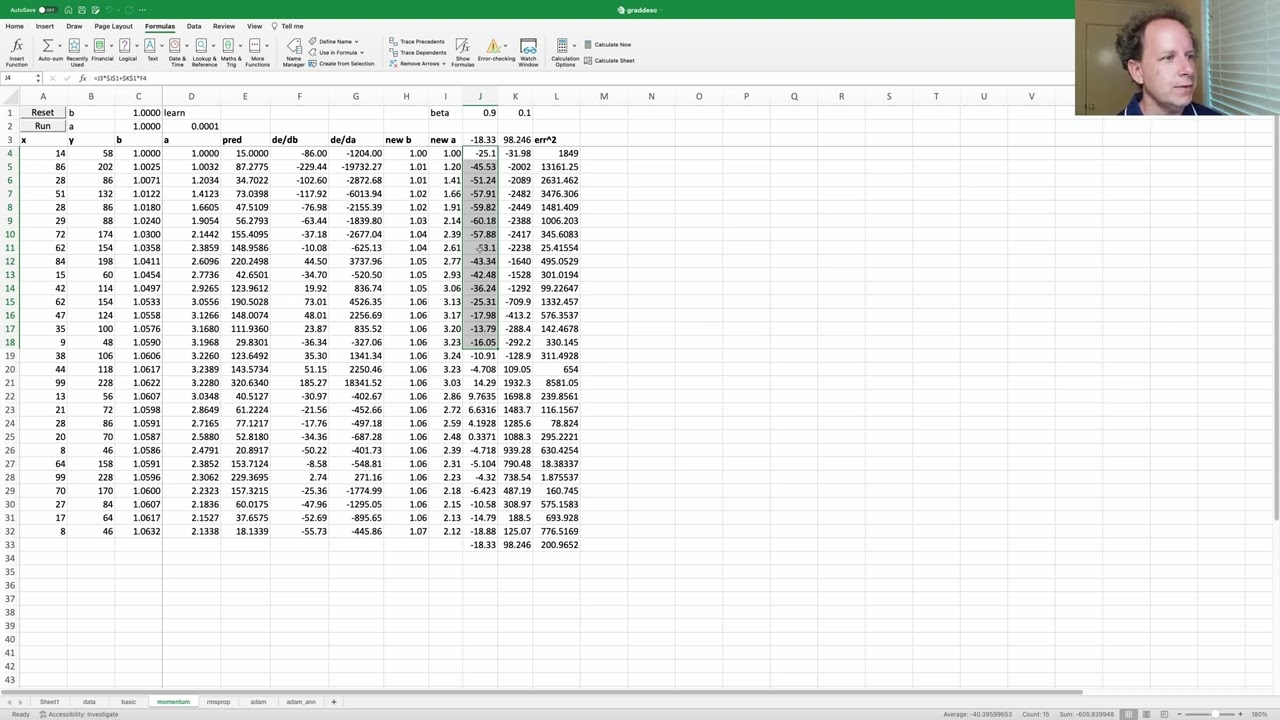
00:10:54.960 | that that is what momentum does so on the next sheet we show momentum and so everything's exactly

00:11:03.040 | the same as the previous sheet but this sheet we didn't bother with the finite differencing we just

00:11:08.000 | have the analytic derivatives which are exactly the same as last time the data is the same as last

00:11:12.720 | time the slope and intercept are the same starting points as last time and this is the

00:11:20.480 | new b and new a that we get but what we do this time

00:11:28.400 | is that we've added a momentum term which we're calling beta

00:11:39.360 | and so the beta is going to these cells here

00:11:44.320 | and what are these cells what what these cells are

00:11:51.200 | is that they're maybe it's most interesting to take this one here

00:11:55.440 | what it's doing is it's taking the gradient and

00:12:08.240 | it's taking the gradient and it's using that to update the weights but it's also taking the

00:12:17.680 | previous update so you can see here the blue one minus 25 so that is going to get multiplied by

00:12:25.600 | 0.9 the momentum and then the derivative is then multiplied by 0.1 so this is momentum which is

00:12:36.320 | getting a little bit of each and so then what we do is we then use that instead of the derivative

00:12:46.560 | to multiply by our learning rate so we keep doing that again and again and again as per usual and

00:12:57.440 | so we've got one column which is calculating the next which is calculating the momentum you know

00:13:02.640 | lerped version of the gradient for both b and for a and so you can see that for this one it's the

00:13:09.040 | same thing you look at what was the previous move and that's going to be 0.9 of what you're going

00:13:17.360 | to use for your momentum version gradient and 0.1 is for this version the momentum gradient

00:13:23.840 | and so then that's again what we're going to use to multiply by the learning rate

00:13:30.800 | and so you can see what happens is when you keep moving in the same direction which here is we're

00:13:36.720 | saying the derivative is negative again and again and again so it gets higher and higher and higher

00:13:42.240 | and get over here and so particularly with this big jump we get we keep getting big jumps because

00:13:50.560 | still we want to then there's still negative gradient negative gradient negative gradient

00:13:54.720 | so if we at so at the end of this our new our b and our a have jumped ahead and so we can click run

00:14:05.040 | and we can click clicking it and you can see that it's moving

00:14:11.120 | you know not super fast but certainly faster than it was before

00:14:19.200 | so if you haven't used vba visual basic for applications before you can hit alt

00:14:24.480 | alt f11 or option f11 to to open it and you may need to go into your preferences

00:14:33.440 | and turn on the developer tools so that you can see it

00:14:37.760 | you can also right click and choose assign macro on a button and you can see what

00:14:46.400 | macro has been assigned so if i hit alt f11 and i can just double or you can just double

00:14:53.520 | click on the sheet name and it'll open it up and you can see that this is exactly the same

00:14:59.760 | as the previous one there's no difference here

00:15:03.680 | oh one difference is that to keep track of momentum

00:15:09.280 | at the very very end so i've got my momentum values going all the way down

00:15:15.360 | the very last momentum i copy back up to the top h epoch so that we don't lose track of our kind

00:15:22.800 | of optimizer state if you like okay so that's what momentum looks like so yeah if you're kind of a

00:15:28.800 | more of a visual person like me you like to see everything laid out in front of you and like to

00:15:32.720 | be able to experiment which i think is a good idea this can be really helpful so rms prop

00:15:44.080 | we've seen and it's very similar to momentum but in this case instead of keeping track of

00:15:49.680 | kind of a lerped moving average an exponential moving average of gradients we're keeping track

00:15:54.400 | of a moving average of gradient squared and then rather than simply adding that you know using

00:16:04.560 | that as the gradient what instead we're doing is we are dividing our gradient by the square root of

00:16:13.680 | that and so remember the reason we were doing that is to say if you know if if the there's very

00:16:23.040 | little variation very little going on in your gradients then you probably want to jump further

00:16:29.120 | so that's rms prop and then finally atom remember was a combination of both

00:16:41.440 | so in atom we've got both the lerped version of the gradient and we've got the lerped version

00:16:49.360 | of the gradient squared and then we do both when we update we're both dividing the gradient by the

00:17:00.960 | square root of the lerped the moving exponentially weighting average moving averages and we're also

00:17:07.920 | using the momentumized version and so again we just go through that each time

00:17:15.120 | and so if i reset run

00:17:20.960 | and so oh wow look at that it jumped up there very quickly because remember we wanted to get to 2

00:17:29.680 | and 30 so just two sets so that's five that's 10 epochs now if i keep running it

00:17:39.280 | it's kind of now not getting closer it's kind of jumping up and down

00:17:45.200 | between pretty much the same values so probably what we'd need to do is decrease the learning

00:17:49.600 | rate at that point and yeah that's pretty good and now it's jumping up and down between the same

00:17:58.480 | two values again so maybe decrease the learning rate a little bit more and i kind of like playing

00:18:02.960 | around like this because it gives me a really intuitive feeling for what training looks like

00:18:08.320 | so i've got a question from our youtube chat which is how is j 33 being initialized so it's it's this

00:18:17.520 | is just what happens is we take the very last cell here well these actually all these last four cells

00:18:24.320 | and we copy them to here as values so this is what those looked like

00:18:29.680 | in the last epoch so if i basically we're going we go copy and then

00:18:38.080 | paste as values and then they this here just refers back to them

00:18:49.120 | as you see and it's interesting that they're kind of you can see how they're exact opposites of

00:18:55.840 | each other which is really you can really see how they're it's it's just fluctuating around

00:19:01.520 | the actual optimum at this point um okay thank you to sam whatkins we've now got a nicer sized

00:19:10.960 | editor that's great um where are we adam

00:19:18.080 | okay so with um so with adam basically it all looks pretty much the same except now

00:19:27.760 | we have to copy and paste our both our momentums and our

00:19:34.800 | um squared gradients and of course the slopes and intercepts at the end of each step

00:19:42.080 | but other than that it's just doing the same thing and when we reset it it just sets everything back

00:19:46.720 | to their default values now one thing that occurred to me you know when i first wrote this

00:19:53.200 | spreadsheet a few years ago was that manually changing the learning rate seems pretty annoying

00:20:01.360 | now of course we can use a scheduler but a scheduler is something we set up ahead of time

00:20:06.640 | and i did wonder if it's possible to create an automatic scheduler and so i created this

00:20:12.000 | adam annealing tab which honestly i've never really got back to experimenting with so if

00:20:16.880 | anybody's interested they should check this out um what i did here was i

00:20:22.800 | used exactly the same spreadsheet as the adam spreadsheet but i added an extra after i do the

00:20:32.560 | step i added an extra thing which is i automatically decreased the learning rate

00:20:38.240 | in a certain situation and the situation in which i in which i decreased it was i kept track of the

00:20:45.120 | average of the um squared gradients and anytime the average of the squared gradients decreased

00:20:52.960 | during an epoch i stored it so i basically kept track of the the lowest squared gradients we had

00:21:02.560 | and then what i did was if we got a if that resulted in the gradients the squared gradients

00:21:17.520 | average halving then i would decrease the learning rate by

00:21:28.640 | then i would decrease the learning rate by a factor of four so i was keeping track of this

00:21:33.280 | gradient ratio now when you see a range like this you can find what that's referring to

00:21:38.400 | by just clicking up here and finding gradient ratio and there it is and you can see that it's

00:21:46.640 | equal to the ratio between the average of the squared gradients versus the minimum that we've

00:21:52.640 | seen so far um so this is kind of like my theory here was thinking that yeah basically as you

00:22:02.000 | train you kind of get into flatter more stable areas and as you do that that's a sign

00:22:11.200 | that you know you might want to decrease your learning rate so uh yeah if i try that if i hit

00:22:19.040 | run again it jumps straight to a pretty good value but i'm not going to change the learning rate

00:22:24.000 | manually i just press run and because it's changed the learning rate automatically now

00:22:27.600 | and if i keep hitting run without doing anything

00:22:31.520 | look at that it's got pretty good hasn't it and the learning rates got lower and lower

00:22:38.080 | and we basically got almost exactly the right answer so yeah that's a little experiment i tried

00:22:44.800 | so maybe some of you should try experiments around whether you can create a an automatic annealer

00:22:53.360 | using the um using mini ai i think that would be fun

00:22:58.560 | so that is an excellent segue into our notebook because we are going to talk about annealing now

00:23:10.240 | so we've seen it manually before um where we've just where we've just decreased the learning rate

00:23:17.760 | in a notebook and like ran a second cell um and we've seen something in excel um but let's look

00:23:25.360 | at what we generally do in pytorch so we're still in the same notebook as last time the accelerated

00:23:32.960 | SGD notebook um and now that we've reimplemented all the main optimizers that t equal tend to use

00:23:41.680 | most of the time from scratch we can use pytorches of course um so let's see look look now at how we

00:23:52.080 | can do our own learning rate scheduling or annealing within the mini ai framework

00:24:00.960 | now we've seen when we implemented the learning rate finder um that that we saw how to

00:24:09.280 | create something that adjusts the learning rate so just to remind you

00:24:14.560 | this was all we had to do so we had to go through the optimizers parameter groups and in each group

00:24:24.480 | set the learning rate to times equals some model player if we're just that was for the learning

00:24:29.040 | rate finder um so since we know how to do that we're not going to bother reimplementing all the

00:24:37.120 | schedulers from scratch um because we know the basic idea now so instead what we're going to have

00:24:42.320 | do is have a look inside the torch dot optim dot lr scheduler module and see what's defined in there

00:24:49.440 | so the lr scheduler module you know you can hit dot tab and see what's in there

00:24:58.240 | but something that i quite like to do is to use dir because dir lr scheduler is a nice little

00:25:06.640 | function that tells you everything inside a python object and this particular object is

00:25:14.640 | a module object and it tells you all the stuff in the module um when you use the dot version

00:25:21.120 | tab it doesn't show you stuff that starts with an underscore by the way because that stuff's

00:25:26.800 | considered private or else dir does show you that stuff now i can kind of see from here that the

00:25:31.760 | things that start with a capital and then a small letter look like the things we care about we

00:25:39.120 | probably don't care about this we probably don't care about these um so we can just do a little

00:25:44.080 | list comprehension that checks that the first letter is an uppercase and the second letter is

00:25:48.240 | lowercase and then join those all together with a space and so here is a nice way to get a list of

00:25:54.160 | all of the schedulers that pytorch has available and actually um i didn't couldn't find such a list

00:26:00.640 | on the pytorch website in the documentation um so this is actually a handy thing to have available

00:26:06.240 | so here's various schedulers we can use and so i thought we might experiment with using

00:26:18.240 | cosine annealing um so before we do we have to recognize that these um pytorch schedulers work

00:26:29.600 | with pytorch optimizers not with of course with our custom sgd class and pytorch optimizers have

00:26:35.600 | a slightly different api and so we might learn how they work so to learn how they work we need

00:26:40.880 | an optimizer um so some one easy way to just grab an optimizer would be to create a learner

00:26:47.840 | just kind of pretty much any old random learner and pass in that single batch callback that we

00:26:53.760 | created do you remember that single batch callback single batch it just after batch it

00:27:01.600 | cancels the fit so it literally just does one batch um and we could fit and from that we've

00:27:09.920 | now got a learner and an optimizer and so we can do the same thing we can do our optimizer to see

00:27:17.040 | what attributes it has this is a nice way or of course just read the documentation in pytorch this

00:27:21.280 | one is documented um i think showing all the things it can do um as you would expect it's

00:27:26.480 | got the step and the zero grad like we're familiar with um or you can just if you just hit um opt

00:27:34.720 | um so you can uh the optimizers in pytorch do actually have a a repra as it's called which

00:27:42.480 | means you can just type it in and hit shift enter and you can also see the information about it this

00:27:46.720 | way now an optimizer it'll tell you what kind of optimizer it is and so in this case the default

00:27:53.280 | optimizer um for a learner when we created it we decided was uh optim.sgd.sgd so we've got an sgd

00:28:02.960 | optimizer and it's got these things called parameter groups um what are parameter groups well

00:28:09.280 | parameter groups are as it suggests they're groups of parameters and in fact we only have

00:28:15.440 | one parameter group here which means all of our parameters are in this group um so let me kind of

00:28:22.720 | try and show you it's a little bit confusing but it's kind of quite neat so let's grab all of our

00:28:28.320 | parameters um and that's actually a generator so we have to turn that into an iterator and call

00:28:34.960 | next and that will just give us our first parameter okay now what we can do is we can then

00:28:42.880 | check the state of the optimizer and the state is a dictionary and the keys are parameter tensors

00:28:53.200 | so this is kind of pretty interesting because you might be i'm sure you're familiar with dictionaries

00:28:57.120 | i hope you're familiar with dictionaries but normally you probably use um numbers or strings

00:29:03.120 | as keys but actually you can use tensors as keys and indeed that's what happens here if we look at

00:29:08.640 | param it's a tensor it's actually a parameter which remember is a tensor which it knows to

00:29:16.960 | to require grad and to to list in the parameters of the module and so we're actually using that

00:29:25.680 | to index into the state so if you look at up.state it's a dictionary where the keys are parameters

00:29:35.520 | now what's this for well what we want to be able to do is if you think back to

00:29:40.880 | this we actually had each parameter we have state for it we have the average of the gradients or the

00:29:49.840 | exponentially way to moving average gradients and of squared averages and we actually stored them

00:29:54.240 | as attributes um so pytorch does it a bit differently it doesn't store them as attributes

00:30:00.400 | but instead it it the the optimizer has a dictionary where you can look at where you can

00:30:06.480 | index into it using a parameter

00:30:09.920 | and that gives you the state and so you can see here it's got a this is the this is the

00:30:20.960 | exponentially weighted moving averages and both because we haven't done any training yet and

00:30:26.000 | because we're using non-momentum std it's none but that's that's how it would be stored so this

00:30:32.160 | is really important to understand pytorch optimizers i quite liked our way of doing it

00:30:38.080 | of just storing the state directly as attributes but this works as well and it's it's it's fine

00:30:45.840 | you just have to know it's there and then as i said rather than just having parameters

00:30:53.760 | so we in sgd stored the parameters directly but in pytorch those parameters can be put into groups

00:31:06.560 | and so since we haven't put them into groups the length of param groups is one there's just one

00:31:12.720 | group so here is the param groups and that group contains all of our parameters

00:31:23.200 | okay so pg just to clarify here what's going on pg is a dictionary it's a parameter group

00:31:34.320 | and to get the keys from a dictionary you can just listify it that gives you back the keys

00:31:41.760 | and so this is one quick way of finding out all the keys in a dictionary so that you can see all

00:31:46.880 | the parameters in the group and you can see all of the hyper parameters the learning rate

00:31:52.880 | the momentum weight decay and so forth

00:31:55.760 | so that gives you some background about

00:32:02.400 | about what's what's going on inside an optimizer so seva asks isn't indexing by a tensor just like

00:32:13.840 | passing a tensor argument to a method and no it's not quite the same because this is this is state

00:32:20.640 | so this is how the optimizer stores state about the parameters it has to be stored somewhere

00:32:28.800 | for our homemade mini ii version we stored it as attributes on the parameter

00:32:33.920 | but in the pytorch optimizers they store it as a dictionary so it's just how it's stored

00:32:42.640 | okay so with that in mind let's look at how schedulers work so let's create a cosine annealing

00:32:49.600 | scheduler so a scheduler in pytorch you have to pass it the optimizer and the reason for that

00:32:56.240 | is we want to be able to tell it to change the learning rates of our optimizer so it needs to

00:33:01.360 | know what optimizer to change the learning rates of so it can then do that for each set of

00:33:06.560 | parameters and the reason that it does it by parameter group is that as we'll learn in a later

00:33:11.360 | lesson for things like transfer learning we often want to adjust the learning rates of the later

00:33:18.080 | layers differently to the earlier layers and actually have different learning rates

00:33:22.080 | and so that's why we can have different groups and the different groups have the different learning

00:33:28.320 | rates mementums and so forth okay so we pass in the optimizer and then if i hit shift tab a

00:33:36.480 | couple of times it'll tell me all of the things that you can pass in and so it needs to know

00:33:41.680 | t max how many iterations you're going to do and that's because it's trying to do one

00:33:48.000 | you know half a wave if you like of the cosine curve so it needs to know how many iterations

00:33:56.080 | you're going to do so it needs to know how far to step each time so if we're going to do 100

00:33:59.680 | iterations so the scheduler is going to store the base learning rate and where did it get that from

00:34:06.720 | it got it from our optimizer which we set a learning rate okay so it's going to steal the

00:34:14.880 | optimizer's learning rate and that's going to be the starting learning rate the base learning rate

00:34:20.640 | and it's a list because there could be a different one for each parameter group we only have one

00:34:24.160 | parameter group you can also get the most recent learning rate from a scheduler which of course

00:34:30.720 | is the same and so i couldn't find any method in pytorch to actually plot a scheduler's learning

00:34:39.040 | rates so i just made a tiny little thing that just created a list set it to the last learning rate of

00:34:46.240 | the scheduler which is going to start at 0.06 and then goes through however many steps you ask for

00:34:51.680 | steps the optimizer steps the scheduler so this is the thing that causes the scheduler to

00:34:58.400 | to adjust its learning rate and then just append that new learning rate to a list of learning

00:35:04.240 | rates and then plot it so that's here's and what i've done here is i've intentionally gone over 100

00:35:11.120 | because i had told it i'm going to do 100 so i'm going over 100 and you can see the learning rate

00:35:16.480 | if we did 100 iterations would start high for a while it would then go down and then it would stay

00:35:23.520 | low for a while and if we intentionally go past the maximum it's actually start going up again

00:35:28.720 | because this is a cosine curve so um one of the main things i guess i wanted to show here is like

00:35:37.680 | what it looks like to really investigate in a repl environment like a notebook

00:35:47.520 | how you know how an object behaves you know what's in it and you know this is something i

00:35:54.160 | would always want to do when i'm using something from an api i'm not very familiar with i really

00:35:59.200 | want to like see what's in it see what they do run it totally independently plot anything i can plot

00:36:06.560 | this is how i yeah like to learn about the stuff i'm working with

00:36:14.000 | um you know data scientists don't spend all of their time just coding you know so that means

00:36:21.040 | we need we can't just rely on using the same classes and apis every day so we have to be

00:36:28.880 | very good at exploring them and learning about them and so that's why i think this is a really

00:36:33.440 | good approach okay so um let's create a scheduler callback so a scheduler callback is something

00:36:43.440 | we're going to pass in the scheduling class but remember then when we go the scheduling callable

00:36:51.200 | actually and remember that when we create the scheduler

00:36:54.480 | we have to pass in the optimizer to to schedule and so before fit that's the point at which we

00:37:05.520 | have an optimizer we will create the scheduling object i like this ghetto it's very australian

00:37:11.680 | so the scheduling object we will create by passing the optimizer into the scheduler callable

00:37:16.320 | and then when we do step then we'll check if we're training and if so we'll step

00:37:34.640 | okay so then what's going to call step is after batch so after batch we'll call step

00:37:42.400 | and that would be if you want your scheduler to update the learning rate every batch

00:37:47.760 | um we could also have a um

00:37:55.280 | an epoch scheduler callback which we'll see later and that's just going to be after epoch

00:38:04.560 | so in order to actually see what the schedule is doing we're going to need to create a new

00:38:14.800 | callback to keep track of what's going on in our learner and i figured we could create a

00:38:20.640 | recorder callback and what we're going to do is we're going to be passing in

00:38:26.400 | the name of the thing that we want to record that we want to keep track of in each batch

00:38:33.840 | and a function which is going to be responsible for grabbing the thing that we want

00:38:38.400 | and so in this case the function here is going to grab from the callback look up its param groups

00:38:47.200 | property and grab the learning rate um where does the pg property come from attribute well before

00:38:54.560 | fit the recorder callback is going to grab just the first parameter group um just so it's like you

00:39:02.320 | got to pick some parameter group to track so we'll just grab the first one and so then um also we're

00:39:08.880 | going to create a dictionary of all the things that we're recording so we'll get all the names

00:39:14.560 | so that's going to be in this case just lr and initially it's just going to be an empty list

00:39:19.520 | and then after batch we'll go through each of the items in that dictionary which in this

00:39:25.120 | case is just lr as the key and underscore lr function as the value and we will append to that

00:39:31.120 | list call that method call that function or callable and pass in this callback and that's why this

00:39:40.000 | is going to get the callback and so that's going to basically then have a whole bunch of you know

00:39:46.160 | dictionary of the results you know of each of these functions uh after each batch um during

00:39:55.200 | training um so we'll just go through and plot them all and so let me show you what that's going to

00:40:01.360 | look like if we um let's create a cosine annealing callable um so we're going to have to use a

00:40:13.680 | partial to say that this callable is going to have t max equal to three times however many many

00:40:21.600 | batches we have in our data loader that's because we're going to do three epochs um and then

00:40:28.800 | we will set it running and we're passing in the batch scheduler with the

00:40:40.080 | scheduler callable and we're also going to pass in our recorder callback saying we want to check

00:40:48.640 | the learning rate using the underscore lr function we're going to call fit um and oh this is actually

00:40:55.040 | a pretty good accuracy we're getting you know close to 90 percent now in only three epochs which is

00:41:00.000 | impressive and so when we then call rec dot plot it's going to call remember the rec is the recorder

00:41:08.320 | callback so it plots the learning rate isn't that sweet so we could as i said we would can do exactly

00:41:19.120 | the same thing but replace after batch with after epoch and this will now become a scheduler which

00:41:25.360 | steps at the end of each epoch rather than the end of each batch so i can do exactly the same

00:41:31.120 | thing now using an epoch scheduler so this time t max is three because we're only going to be

00:41:36.400 | stepping three times we're not stepping at the end of each batch just at the end of each epoch

00:41:40.320 | so that trains and then we can call rec dot plot after trains and as you can see there

00:41:48.400 | it's just stepping three times so you can see here we're really digging in deeply to understanding

00:41:59.200 | what's happening in everything in our models what are all the activations look like what

00:42:03.920 | are the losses look like what do our learning rates look like and we've built all this from scratch

00:42:10.720 | so yeah hopefully that gives you a sense that we can really yeah do a lot ourselves

00:42:18.480 | now if you've done the fastai part one course you'll be very aware of one cycle training which

00:42:27.520 | was from a terrific paper by leslie smith which i'm not sure it ever got published actually

00:42:38.080 | and one cycle training is well let's take a look at it

00:42:45.920 | so we can just replace our scheduler with one cycle learning rate scheduler so that's

00:42:56.720 | in pytorch and of course if it wasn't in pytorch we could very easily just write our own

00:43:00.800 | we're going to make it a batch scheduler and we're going to train this time we're going to do

00:43:07.520 | five epochs so we're going to train a bit longer and so the first thing i'll point out is hooray

00:43:12.880 | we have got a new record for us 90.6 so that's great so and then b you can see here's the plot

00:43:24.720 | and now look two things are being plotted and that's because i've now passed into the recorder

00:43:29.200 | callback a plot of learning rates and also a plot of momentums and momentums it's going to

00:43:35.120 | grip the beta's zero because remember for adam it's called beta zero and beta one is momentum

00:43:42.960 | of the gradients and the momentum of the gradient squared and you can see what the one cycle is

00:43:50.880 | doing is the learning rate is starting very low and going up to high and then down again

00:44:00.320 | but the momentum is starting high and then going down and then up again so what's the theory here

00:44:09.360 | well the the the starting out at a low learning rate is particularly important if you have a

00:44:17.760 | not perfectly initialized model which almost everybody almost always does even though we

00:44:27.600 | spent a lot of time learning to initialize models you know we use a lot of models that get more

00:44:33.920 | complicated and after a while people after a while people learn or figure out how to initialize more

00:44:47.040 | complex models properly so for example this is a very very cool paper in 2019 this team figured out

00:44:59.200 | how to initialize resnets properly we'll be looking at resnets very shortly and they discovered when

00:45:05.120 | they did that they did not need batch norm they could train networks of 10 000 layers

00:45:12.720 | and they could get state-of-the-art performance with no batch norm and there's actually been

00:45:18.000 | something similar for transformers called tfixup that does a similar kind of thing

00:45:30.240 | but anyway it is quite difficult to initialize models correctly most people fail to most people

00:45:38.720 | fail to realize that they generally don't need tricks like warm up and batch norm if they do

00:45:45.520 | initialize them correctly in fact tfixup explicitly looks at this it looks at the difference between

00:45:49.920 | no warm up versus with warm up with their correct initialization versus with normal initialization

00:45:56.160 | and you can see these pictures they're showing are pretty similar actually

00:46:00.080 | log scale histograms of gradients they're very similar to the colorful dimension plots

00:46:05.280 | i kind of like our colorful dimension plots better in some ways because i think they're

00:46:08.640 | easier to read although i think theirs are probably prettier so there you go stufano

00:46:12.880 | there's something to inspire you if you want to try more things with our colorful dimension plots

00:46:18.000 | i think it's interesting that some papers are actually starting to

00:46:21.280 | use a similar idea i don't know if they got it from us or they came up with it independently

00:46:27.120 | doesn't really matter but so that so we do a warm up if our if our if our

00:46:35.680 | network's not quite initialized correctly then starting at a very low learning rate means it's

00:46:41.200 | not going to jump off way outside the area where the weights even make sense and so then you

00:46:47.440 | gradually increase them as the weights move into a part of the space that does make sense

00:46:53.360 | and then during that time while we have low learning rates if they keep moving in the same

00:46:58.640 | direction then with it it's very high momentum they'll move more and more quickly but if they

00:47:03.040 | keep moving in different directions it's just the momentum is going to kind of look at the

00:47:07.840 | underlying direction they're moving and then once you have got to a good part of the weight

00:47:13.600 | space you can use a very high learning rate and with a very high learning rate you wouldn't want

00:47:17.920 | so much momentum so that's why there's low momentum during the time when there's high learning rate

00:47:23.200 | and then as we saw in our spreadsheet which did this automatically as you get closer to

00:47:30.000 | the optimal you generally want to decrease the learning rate and since we're decreasing it again

00:47:35.840 | we can increase the momentum so you can see that starting from random weights we've got a pretty

00:47:42.160 | good accuracy on fashion MNIST with a totally standard convolutional neural network no resonance

00:47:48.400 | nothing else everything built from scratch by hand artisanal neural network training and we've got

00:47:55.120 | 90.6 percent fashion MNIST so there you go all right let's take a seven minute break

00:48:06.480 | and i'll see you back shortly i should warn you you've got a lot more to cover so i hope you're

00:48:15.120 | okay with a long lesson today

00:48:18.880 | okay we're back um i just wanted to mention also something we skipped over here

00:48:29.840 | which uh is this has learn callback um this is more important for the people doing the live

00:48:37.840 | course than the recordings if you're doing the recording you will have already seen this but

00:48:41.840 | since i created learner actually uh peter zappa i don't know how to pronounce your surname sorry peter

00:48:49.440 | um uh pointed out that there's actually kind of a nicer way of of handling learner that um previously

00:48:58.960 | we were putting the learner object itself into self.learn in each callback and that meant we were

00:49:05.280 | using self.learn.model and self.learn.opt and self.learn.all this you know all over the place it was

00:49:10.400 | kind of ugly um so we've modified learner this week um to instead

00:49:19.360 | um pass in when it calls the callback

00:49:27.040 | when in run cbs which is what it calls uh learner calls you might remember is it passes the learner

00:49:40.720 | as a parameter to the method um so now um the learner no longer goes through the callbacks

00:49:48.640 | and sets their dot learn attribute um but instead in your callbacks you have to put

00:49:55.200 | learn as a parameter in all of the method in all of the callback methods so for example

00:50:06.560 | device cb has a before fit so now it's got comma learn here so now this is not self.learn it's just

00:50:13.760 | learn um so it does make a lot of the code um less less yucky to not have all this self.learn.pred

00:50:23.840 | equals self.learn.model self.learn.batch is now just learn. it also is good because you don't

00:50:29.440 | generally want to have um both have the learner um has a reference to the callbacks

00:50:38.400 | but also the callbacks having a reference back to the learner it creates something called a cycle

00:50:44.080 | so there's a couple of benefits there um and that reminds me there's a few other little changes

00:50:55.120 | we've made to the code and i want to show you a cool little trick i want to show you a cool

00:51:02.080 | little trick for how i'm going to find quickly all of the changes that we've made to the code in the

00:51:07.600 | last week so to do that we can go to the course repo and on any repo you can add slash compare

00:51:17.280 | in github and then you can compare across um you know all kinds of different things but one of the

00:51:25.120 | examples they've got here is to compare across different times look at the master branch now

00:51:29.920 | versus one day ago so i actually want the master branch now versus seven days ago so i just hit

00:51:36.400 | this change this to seven and there we go there's all my commits and i can immediately see

00:51:45.280 | the changes from last week um and so you can basically see what are the things i had to do

00:51:52.080 | when i change things so for example you can see here all of my self.learns became learns

00:51:58.880 | i added the nearly that's right i made augmentation

00:52:04.400 | and so in learner i added an lr find oh yes i will show you that one that's pretty fun

00:52:14.880 | so here's the changes we made to run cbs to fit

00:52:20.160 | so this is a nice way i can quickly yeah find out um what i've changed since last time and make sure

00:52:28.480 | that i don't forget to tell you folks about any of them oh yes clean up fit i have to tell you

00:52:34.080 | about that as well okay that's a useful reminder so um the main other change to mention is that

00:52:43.520 | calling the learning rate finder is now easier because i added what's called a patch to the

00:52:51.360 | learner um fast cause patch decorator that's you take a function and it will turn that function

00:53:00.160 | into a method of this class of whatever class you put after the colon so this has created a new

00:53:07.920 | method called lr find or learner dot lr find and what it does is it calls self.fit where self is a

00:53:20.480 | learner passing in however many epochs you set as the maximum you want to check for your learning

00:53:25.360 | rate finder what to start the learning rate at and then it says to use as callbacks the learning

00:53:33.680 | rate finder callback now this is new as well um self dot learn.fit didn't used to have a callbacks

00:53:41.120 | parameter um so that's very convenient because what it does is it adds those callbacks just

00:53:49.680 | during the fit so if you pass in callbacks then it goes through each one and appends it

00:53:57.840 | to self.cb's and when it's finished fitting it removes them again so these are callbacks that

00:54:04.960 | are just added for the period of this one fit which is what we want for a learning rate finder

00:54:09.200 | it should just be added for that one fit um so with this patch in place it says this is all

00:54:16.800 | it's required to do the learning rate finder is now to create your learner and call dot lr find

00:54:23.040 | and there you go bang so patch is a very convenient thing it's um one of these things which you know

00:54:30.320 | python has a lot of kind of like folk wisdom about what is and isn't considered pythonic or

00:54:38.800 | good and a lot of people uh really don't like patching um in other languages it's used very

00:54:46.720 | widely and is considered very good um so i i don't tend to have strong opinions either way about

00:54:53.680 | what's good or what's bad in fact instead i just you know figure out what's useful in a particular

00:54:58.080 | situation um so in this situation obviously it's very nice to be able to add in this additional

00:55:04.720 | functionality to our class so that's what lr find is um and then the only other thing we added to

00:55:12.560 | the learner uh this week was we added a few more parameters to fit fit used to just take the number

00:55:18.480 | of epochs um as well as the callbacks parameter it now also has a learning rate parameter and

00:55:25.120 | so you've always been able to provide a learning rate to um the constructor but you can override

00:55:31.600 | the learning rate for one fit so if you pass in the learning rate it will use it if you pass it

00:55:39.840 | in and if you don't it'll use the learning rate passed into the constructor and then i also added

00:55:46.000 | these two booleans to say when you fit do you want to do the training loop and do you want to

00:55:52.080 | do the validation loop so by default it'll do both and you can see here there's just an if train do

00:55:57.760 | the training loop if valid do the validation loop um i'm not even going to talk about this but if

00:56:05.600 | you're interested in testing your understanding of decorators you might want to think about why it

00:56:10.960 | is that i didn't have to say with torch.nograd but instead i called torch.nograd parentheses

00:56:17.360 | function that will be a very if you can get to a point that you understand why that works and what

00:56:22.880 | it does you'll be on your way to understanding decorators better okay

00:56:31.280 | so that is the end of excel sgd

00:56:36.640 | resnets okay so we are up to 90 point what was it three percent uh yeah let's keep track of this

00:56:50.080 | oh yeah 90.6 percent is what we're up to okay so to remind you the model

00:57:00.880 | um actually so we're going to open 13 resnet now um and we're going to do the usual important setup

00:57:11.840 | initially and the model that we've been using is the same one we've been using for a while

00:57:24.160 | which is that it's a convolution and an activation and an optimal optional batch norm

00:57:33.600 | and uh in our models we were using batch norm and applying our weight initialization the kiming

00:57:44.880 | weight initialization and then we've got comms that take the channels from 1 to 8 to 16 to 32 to 64

00:57:52.560 | and each one's dried two and at the end we then do a flatten and so that ended up with a one by one

00:57:59.440 | so that's been the model we've been using for a while so the number of layers is one

00:58:07.600 | two three four so four four convolutional layers with a maximum of 64 channels in the last one

00:58:20.480 | so can we beat 90.9 about 90 and a half

00:58:24.400 | 90.6 can we beat 90.6 percent so before we do a resnet i thought well let's just see if we can

00:58:33.760 | improve the architecture thoughtfully so generally speaking um more depth and more channels gives the

00:58:43.440 | neural net more opportunity to learn and since we're pretty good at initializing our neural nets

00:58:48.000 | and using batch norm we should be able to handle deeper so um one thing we could do

00:58:55.680 | is we could let's just remind ourselves of the

00:59:00.160 | previous version so we can compare

00:59:08.080 | is we could have our go up to 128 parameters now the way we do that is we could make our

00:59:18.800 | very first convolutional layer have a stride of one so that would be one that goes from

00:59:25.040 | the one input channel to eight output channels or eight filters if you like so if we make it a

00:59:32.640 | stride of one then that allows us to have one extra layer and then that one extra layer could

00:59:39.840 | again double the number of channels and take us up to 128 so that would make it uh deeper and

00:59:45.840 | effectively wider as a result um so we can do our normal batch norm 2d and our new one cycle

00:59:54.320 | learning rate with our scheduler um and the callbacks we're going to use is the device call back

01:00:01.840 | our metrics our progress bar and our activation stats looking for general values and i won't

01:00:09.600 | what have you watched them train because that would be kind of boring but if i do this with

01:00:14.080 | this deeper and eventually wider network this is pretty amazing we get up to 91.7 percent

01:00:22.000 | so that's like quite a big difference and literally the only difference to our previous model

01:00:27.840 | is this one line of code which allowed us to take this instead of going from one to 64 it goes from

01:00:36.080 | eight to 128 so that's a very small change but it massively improved so the error rate's gone down

01:00:41.840 | by a temp you know about well over 10 percent relatively speaking um in terms of the error rate

01:00:47.840 | so there's a huge impact we've already had um again five epochs

01:00:56.240 | so now what we're going to do is we're going to make it deeper still

01:00:59.040 | but it gets there becomes a point um so chiming her at our noted that there comes a point where

01:01:08.800 | making neural nets deeper stops working well and remember this is the guy who created the

01:01:15.520 | initializer that we know and love and he pointed out that even with that good initialization

01:01:23.440 | there comes a time where adding more layers becomes problematic and he pointed out something

01:01:29.520 | particularly interesting he said let's take a 20-layer neural network this is in a paper

01:01:36.240 | called deep deep residue learning for image recognition that introduced resnets so let's

01:01:40.480 | take a 20-layer network and train it for a few what's that tens of thousands of iterations

01:01:50.000 | and track its test error okay and now let's do exactly the same thing on a 56-layer

01:01:56.400 | identical otherwise identical but deeper 56-layer network and he pointed out that the 56-layer

01:02:02.400 | network had a worse error than the 20-layer and it wasn't just a problem of generalization because

01:02:08.080 | it was worse on the training set as well now the insight that he had is if you just set the

01:02:24.000 | additional 36 layers to just identity you know identity matrices they should they would do

01:02:31.920 | nothing at all and so a 56-layer network is a superset of a 20-layer network so it should be

01:02:40.320 | at least as good but it's not it's worse so clearly the problem here is something about

01:02:47.200 | training it and so him and his team came up with a really clever insight which is

01:02:56.800 | can we create a 56-layer network which has the same training dynamics as a 20-layer network or even

01:03:06.080 | less and they realized yes you can what you could do is you could add something called

01:03:16.880 | a shortcut connection and basically the idea is that normally when we have you know our

01:03:28.640 | inputs coming into our convolution so let's say that's that was our inputs and here's our convolution

01:03:38.560 | and here's our outputs now if we do this 56 times that's a lot of stacked up convolutions

01:03:50.640 | which are effectively matrix multiplications with a lot of opportunity for you know gradient

01:03:55.200 | explosions and all that fun stuff so how could we make it so that we have convolutions but

01:04:05.840 | with the training dynamics of a much shallower network and

01:04:10.080 | here's what he did he said let's actually put two comms in here

01:04:24.720 | to make it twice as deep because we are trying to make things deeper but then

01:04:34.080 | let's add what's called a skip connection where instead of just being out equals so this is conv1

01:04:44.240 | this is conv2 instead of being out equals and there's a you know assume that these include

01:04:50.080 | activation functions equals conv2 of conv1 of in right instead of just doing that let's make

01:05:02.560 | it conv2 of conv1 of in plus in now if we initialize these at the first to have weights of

01:05:18.480 | zero then initially this will do nothing at all it will output zero and therefore

01:05:29.440 | at first you'll just get out equals in which is exactly what we wanted right we actually want

01:05:37.680 | to to to for it to be as if there is no extra layers and so this way we actually end up

01:05:48.720 | with a network which can which can be deep but also at least when you start training behaves

01:05:56.560 | as if it's shallow it's called a residual connection because if we subtract in from both sides

01:06:05.440 | out then we would get out minus in equals conv1 of conv2 of in in other words

01:06:16.800 | the difference between the end point and the starting point which is the residual and so

01:06:25.280 | another way of thinking about it is that this is calculating a residual

01:06:32.000 | so there's a couple of ways of thinking about it and so this this thing here

01:06:39.840 | is called the res block or res net block

01:06:50.080 | okay so Sam Watkins has just pointed out the confusion here which is that this only works

01:06:58.720 | if let's put the minus in back and put it back over here

01:07:05.600 | this only works if you can add these together now if conv1 and conv2 both have the same number of

01:07:16.160 | channels as in the same number of filters same number of filters and they also have stride1

01:07:25.120 | then that will work fine you'll end up that will be exactly the same output shape as the

01:07:33.760 | input shape and you can add them together but if they are not the same then you're in a bit of

01:07:44.240 | trouble so what do you do and the answer which um timing her et al came up with is to add a conv

01:07:55.120 | on in as well but to make it as simple as possible we call this the identity conv it's not really an

01:08:06.080 | identity anymore but we're trying to make it as simple as possible so that we do as little to

01:08:11.840 | mess up these training dynamics as we can and the simplest possible convolution is a one by one

01:08:18.960 | filter block a one by one kernel i guess we should call it

01:08:23.360 | a one by one kernel size

01:08:27.760 | and using that and we can also add a stride or whatever if we want to so let me show you the code

01:08:39.440 | so we're going to create something called a conv block okay and the conv block is going to do

01:08:45.600 | the two comms that's going to be a conv block okay so we've got some number of input filters

01:08:52.320 | some number of output filters some stride some activation functions possibly a normalization

01:08:59.520 | and possibly and some some kernel shape some kernel size so um the second conv is actually

01:09:10.320 | going to go from output filters to output filters because the first conv is going to be from input

01:09:18.000 | filters to output filters so by the time we get to the second conv it's going to be nf to nf

01:09:25.440 | the first conv we will set stride one and then the second conv will have the requested stride

01:09:32.080 | and so that way the two comms back to back are going to overall have the requested stride

01:09:36.960 | so this way the combination of these two comms is going to eventually is going to take us from ni

01:09:42.640 | to nf in terms of the number of filters and it's going to have the stride that we requested

01:09:47.360 | so it's going to be a the conv block is a sequential block consisting of a convolution

01:09:54.800 | followed by another convolution each one with a requested kernel size

01:09:58.720 | and requested activation function and the requested normalization layer

01:10:06.400 | the second conv won't have an activation function i'll explain why in a moment

01:10:10.880 | and so i mentioned that one way to make this as if it didn't exist would be to set the convolutional

01:10:22.320 | weights to zero and the biases to zero but actually we would we would like to have

01:10:27.200 | you know correctly randomly initialized weights so instead what we can do is if you're using

01:10:34.800 | batch norm we can initialize this conv two one will be the batch norm layer we can initialize

01:10:41.360 | the batch norm weights to zero now if you've forgotten what that means go back and have a

01:10:46.880 | look at our implementation from scratch of batch norm because the batch norm weights is the thing

01:10:51.360 | we multiply by so do you remember the batch norm we we subtract the exponential moving average

01:11:00.640 | mean we divide by the exponential moving average standard deviation but then we add back the the

01:11:08.240 | kind of the the the batch norms bias layer and we multiply by the batch norms weights

01:11:13.680 | well the way around multiplied by weights first so if we set the batch norm layers weights to zero

01:11:19.840 | we're multiplying by zero and so this will cause the initial conv block output to be just all zeros

01:11:27.360 | and so that's going to give us what we wanted is that nothing's happening here so we just end up

01:11:35.120 | with the input with this possible id conv so a res block is going to contain those convolutions

01:11:45.600 | in the convolution block we just discussed right and then we're going to need this id conv

01:11:50.560 | so the id conv is going to be a no op so that's nothing at all if the number of channels in is

01:11:58.800 | equal to the number of channels out but otherwise we're going to use a convolution with a kernel

01:12:04.080 | size of one and a stride of one and so that is going to you know is as with as little work as

01:12:11.520 | possible change the number of filters so that they match also what if the stride's not one

01:12:19.760 | well if the stride is two actually i'm actually this isn't going to work for any stride this only

01:12:25.040 | works for a stride of two if there's a stride of two we will simply average using average pooling

01:12:31.280 | so this is just saying take the mean of every set of two items in the grid so we'll just take the

01:12:43.920 | mean so we we so we basically have here pool of id conv of in if the if the stride is two and if

01:12:57.280 | the filtered number is changed and so that's the minimum amount of work so here it is here is the

01:13:03.760 | forward pass we get our input and on the identity connection we call pool and if stride is one

01:13:12.480 | that's a no op so do nothing at all we do id conv and if the number of filters has not changed

01:13:18.960 | that's also a no op so this is this is just the input in that situation and then we add that

01:13:26.640 | to the result of the convs and here's something interesting we then apply the activation function

01:13:32.400 | to the whole thing okay so that way i wouldn't say this is like the only way you can do it

01:13:40.000 | but this is this is a way that works pretty well is to apply the activation function to the result

01:13:46.400 | of the whole the whole res net block and that's why i didn't add activation function to the second

01:13:55.760 | conv so that's a res block so it's not a huge amount of code right and so now i've literally

01:14:04.960 | copied and pasted our get model but everywhere that previously we had a conv i've just replaced

01:14:09.680 | it with res block in fact let's have a look get model okay so previously

01:14:25.040 | we started with conv one to eight now we do res block one to eight stride one stride one

01:14:32.240 | then we added con from number of filters i and number of filters i plus one now it's

01:14:36.640 | res block from number of filters number of filters i plus one okay so it's exactly the same

01:14:40.560 | one change i have made though is i mean it doesn't actually make any difference at all i think it's

01:14:51.280 | mathematically identical is previously the very last conv at the end went from the you know 128

01:14:58.960 | channels down to the 10 channels followed by flatten but this conv is actually working on a one by one

01:15:08.000 | input so you know an alternate way but i think makes it clearer is flatten first and then use

01:15:14.720 | a linear layer because a conv on a one by one input is identical to a linear layer and if that

01:15:21.600 | doesn't immediately make sense that's totally fine but this is one of those places where you

01:15:26.000 | should pause and have a little stop and think about why a conv on a one by one is the same and maybe

01:15:32.240 | go back to the excel spreadsheet if you like or the the python from scratch conv we did because

01:15:38.480 | this is a very important insight so i think it's very useful with a more complex model like this

01:15:44.400 | to take a good old look at it to see exactly what the inputs and outputs of each layer is

01:15:51.280 | so here's a little function called print shape which takes the things that a hook takes

01:15:55.520 | and we will print out for each layer the name of the class the shape of the input and the shape

01:16:04.560 | of the output so we can get our model create our learner and use our handy little hooks context

01:16:11.840 | manager we built an earlier lesson and call the print shape function and then we will call fit

01:16:18.720 | for one epoch just doing the evaluation of the training and if we use the single batch callback

01:16:25.200 | it'll just do a single batch put put pass it through and that hook will as you see print out

01:16:31.760 | each layer the inputs shape and the output shape

01:16:42.320 | so you can see we're starting with an input of batch size of 1024 one channel 28 by 28

01:16:49.920 | our first res block was dried one so we still end up with 28 by 28 but now we've got eight channels

01:16:54.880 | and then we gradually decrease the grid size to 14 to 7 to 4 to 2 to 1 as we gradually increase

01:17:03.520 | the number of channels we then flatten it which gets rid of that one by one which allows us then

01:17:11.280 | to do linear to go under the 10 and then there's some discussion about whether you want a batch

01:17:20.880 | norm at the end or not i was finding it quite useful in this case so we've got a batch norm at

01:17:26.000 | the end i think this is very useful so i decided to create a patch for learner called summary

01:17:35.760 | that would do basically exactly the same thing but it would do it as a markdown table

01:17:41.840 | okay so if we create a train learner with our model and um call dot summary this method is now

01:17:57.840 | available because it's been patched that method into the learner and it's going to do exactly the

01:18:04.880 | same thing as our print but it does it more prettily by using a markdown table if it's in

01:18:10.400 | a notebook otherwise it'll just print it um so fast call has a handy thing for keeping track if

01:18:15.520 | you're in a notebook and in a notebook to make something markdown you can just use ipython dot

01:18:20.800 | display dot markdown as you see um and the other thing that i added as well as the input and the

01:18:27.280 | output is i thought let's also add in the number of parameters so we can calculate that as we've

01:18:34.080 | seen before by summing up the number of elements for each parameter in that module and so then i've

01:18:42.880 | kind of kept track of that as well so that at the end i can also print out the total number of

01:18:47.520 | parameters so we've got a 1.2 million parameter model and you can see that there's very few

01:18:56.080 | parameters here in the input nearly all the parameters are actually in the last layer

01:19:02.800 | why is that well you might want to go back to our excel convolutional spreadsheet to see this

01:19:07.920 | you have a parameter for every input channel you have a set of parameters

01:19:18.160 | they're all going to get added up across each of the three by three in the kernel

01:19:27.200 | and then that's going to be done for every output filter every output channel that you want so

01:19:33.760 | that's why you're going to end up with um in fact let's take a look

01:19:39.600 | maybe let's create let's just grab some particular one so create our model

01:19:52.720 | and so we'll just have a look at

01:20:00.240 | the sizes and so you can see here there is this 256 by 256 by three by three so that's a lot of

01:20:18.960 | parameters okay so we can call lrfind on that and get a sense of what kind of learning rate to use

01:20:31.280 | so i chose 2enag2 so 0.02 this is our standard learning thing you don't have to watch it train

01:20:39.280 | i've just trained it and so look at this by using resnet we've gone up from 91.7

01:20:48.160 | this just keeps getting better 92.2 in 5 epochs so that's pretty nice

01:20:54.320 | and you know this resnet is not anything fancy it's it's the simplest possible res block right

01:21:05.600 | the model is literally copied and pasted from before and replaced each place it said conv with

01:21:10.560 | res block but we've just been thoughtful about it you know and here's something very interesting

01:21:16.960 | we can actually try lots of other resnets by grabbing tim so that's ross weitman's pie torch

01:21:22.960 | image model library and if you call tim.listmodels star resnet star there's a lot of resnets and i

01:21:35.680 | tried quite a few of them now one thing that's interesting is if you actually look at the source

01:21:43.440 | code for tim you'll see that the various different resnets like resnet 18 resnet 18 d resnet 10 d

01:21:56.720 | they're defined in a very nice way using this very elegant configuration you can see exactly

01:22:03.920 | what's different so there's basically only if one line of code different between each different type

01:22:08.880 | of resnet for the main resnets and so what i did was i tried all the tim models i could find

01:22:16.400 | and i even tried importing the underlying things and building my own resnets from those pieces

01:22:24.480 | and the best i found was the resnet 18 d and if i train it in exactly the same way

01:22:34.560 | i got to 92 percent and so the interesting thing is you'll see that's less than our 92.2 and it's

01:22:41.040 | not like i tried lots of things to get here this is the very first thing i tried where else this

01:22:45.760 | resnet 18 d was after trying lots lots of different tim models and so what this shows

01:22:51.200 | is that the just thoughtfully designed kind of basic architecture goes a very long way

01:23:00.400 | it's actually better for this problem than any of the pytorch image model models

01:23:08.640 | resnets that i could try that i could find so i think that's quite quite amazing actually it's

01:23:18.320 | really cool you know and it shows that you can create a state-of-the-art architecture

01:23:24.560 | just by using some common sense you know so i hope that's uh i hope that's yeah hope that's

01:23:31.040 | encouraging so anyway so we're up to 92.2 percent we're not done yet

01:23:39.520 | because we haven't even talked about data augmentation

01:23:47.440 | all right so let's keep going

01:23:52.640 | so we're going to make everything the same as before but before we do data augmentation

01:23:59.440 | we're going to try to improve our model even further if we can so i said it was kind of

01:24:06.480 | not constructed with any great care and thought really like in terms of like this resnet we just

01:24:13.440 | took the convnet and replaced it with a resnet so it's effectively twice as deep because each conv

01:24:20.240 | block has two convolutions but resnets train better than convnets so surely we could go deeper

01:24:29.840 | and wider still so i thought okay how could we go wider and i thought well let's take our model

01:24:43.120 | and previously we were going from eight up to 256 what if we could get up to 512

01:24:50.000 | and i thought okay well one way to do that would be to make our very first res block not have a

01:24:58.240 | kernel size of three but a kernel size of five so that means that each grid is going to be five by

01:25:04.800 | five that's going to be 25 inputs so i think it's fair enough then to have 16 outputs so if i use a

01:25:11.360 | kernel size of five 16 outputs then that means if i keep doubling as before i'm going to end up at

01:25:18.000 | 512 rather than 256 okay so that's the only change i made was to add k equals five here

01:25:30.240 | and then change to double all the sizes um and so if i train that wow look at this 92.7 percent

01:25:42.560 | so we're getting better still um and again it wasn't with lots of like trying and failing and

01:25:51.040 | whatever it was just like saying well this just makes sense and the first thing i tried it just

01:25:55.120 | it just worked you know we're just trying to use these sensible thoughtful approaches okay next

01:26:02.160 | thing i'm going to try isn't necessarily something to make it better but it's something to make our

01:26:06.640 | res net more flexible our current res net is a bit awkward in that the number of stride two layers

01:26:15.440 | has to be exactly big enough that the last of them

01:26:24.160 | that the last of them ends up with a one by one output so you can flatten it and do the linear

01:26:30.800 | so that's not very flexible because you know what if you've got something you know for different

01:26:35.680 | size uh 28 by 28 is a pretty small image so to to kind of make that necessary i've created a get

01:26:45.120 | model two um which goes less far it has one less layer so it only goes up to 256 despite starting

01:26:53.920 | at 16 and so because it's got one less layer that means that it's going to end up at the two by two

01:27:01.600 | not the one by one so what do we do um well we can do something very straightforward

01:27:08.000 | which is we can take the mean over the two by two and so if we take the mean over the two by two

01:27:16.560 | that's going to give us a mean over the two by two it's going to give us batch size by channels

01:27:23.360 | output which is what we can then put into our linear layer so this is called this ridiculously

01:27:30.960 | simple thing is called a global average pooling layer and that's the that's the keras term uh in

01:27:37.360 | pie torch it's basically the same it's called an adaptive average pooling layer um but in it in

01:27:43.440 | pie torch you can cause it to have an output other than one by one um but nobody ever really uses it

01:27:51.360 | that way um so they're basically the same thing um this is actually a little bit more convenient

01:27:56.080 | than the pie torch version because you don't have to flatten it um so this is global average

01:28:01.680 | pooling so you can see here after our last res block which gives us a two by two output we have

01:28:07.280 | global average pool and that's just going to take the mean and then we can do the linear batch norm

01:28:15.120 | as usual so um i wanted to improve my summary patch to include not only the number of parameters

01:28:26.480 | but also the approximate number of mega flops so a flop is a floating operation per second a

01:28:35.520 | floating point operation per second um i'm not going to promise my calculation is exactly right

01:28:41.440 | i think the basic idea is right um i just basically actually calculated it's not really flops actually

01:28:48.000 | counted the number of multiplications um so this is not perfectly accurate but it's pretty indicative

01:28:54.240 | i think um so this is the same summary i had before but i had an added an extra thing which

01:29:00.160 | is a flops function where you pass in the weight matrix and the height and the width of your grid

01:29:07.840 | now if the number of dimensions of the weight matrix is less than three then we're just doing

01:29:14.560 | like a linear layer or something so actually just the number of elements is the number of flops

01:29:19.600 | because it's just a matrix multiply but if you're doing a convolution so the dimension is four

01:29:27.440 | then you actually do that matrix multiply for everything in the height by width grid

01:29:32.400 | so that's how i calculate this kind of flops uh equivalent number so um

01:29:40.480 | okay so if i run that on this model we can now see our number of parameters

01:29:52.320 | compared to the resnet model has gone from uh 1.2 million up to 4.9 million and the reason why is

01:30:02.720 | because we've got this um we've got this res block it gets all the way up to 512 and the way we did

01:30:16.560 | this um is we made that a stride one layer um so that's why you can see here it's gone two two and

01:30:24.560 | it stayed at two two so i wanted to make it as similar as possible to the last ones it's got

01:30:28.480 | you know the same 512 final number of channels and so most of the parameters are in that last

01:30:34.640 | block for the reason we just discussed um interestingly though it's not as clear for

01:30:42.560 | the mega flops you know it it is the greatest of them but you know in terms of number of parameters

01:30:49.520 | i think this has more parameters than the other ones added together by a lot but that's not true

01:30:53.840 | of mega flops and that's because this first layer has to be done 28 by 28 times whereas this layer

01:31:02.880 | only has to be done two by two times anyway so i tried uh training that uh and got pretty similar

01:31:11.120 | result 92.6 um and that kind of made me think oh let's fiddle around with this a little bit more

01:31:19.520 | um to see like what kind of things would reduce the number of parameters and the mega flops

01:31:25.440 | the reason you care about reducing the number of parameters is that it has uh lower memory

01:31:30.400 | requirements and the reason you require want to reduce the number of flops is it's less compute

01:31:40.160 | so in this case what i've done here

01:31:44.880 | is i've removed this line of code so i've removed the line of code that takes it up to 512

01:31:57.040 | so that means we don't have this layer anymore and so the number of parameters has gone down from

01:32:02.560 | 4.9 million down to 1.2 million um not a huge impact on the mega flops but a huge impact on

01:32:10.400 | the parameters we've reduced it by like two-thirds or three-quarters or something

01:32:14.400 | by getting rid of that and you can see that the um if we take the very first resnet block

01:32:28.560 | the number of parameters is you know um why is it this 5.3 mega flops it's because

01:32:34.960 | although the very first one starts with just one channel the first conv remember our resnet blocks

01:32:40.720 | have two comms so the second conv is going to be a 16 by 16 by 5 by 5 and again i'm partly doing

01:32:46.960 | this to show you the actual details of this architecture but i'm partly showing it so that

01:32:51.200 | you can see how to investigate exactly what's going on in your models i really want you to try these

01:32:58.240 | so if we train that one interestingly even though it's only a quarter or something of the size

01:33:05.440 | we get the same accuracy 92.7

01:33:09.920 | so that's interesting um can we make it faster well at this point this is the obvious place to

01:33:21.280 | look at is this first resnet block because that's where the mega flops are and as i said the reason

01:33:27.280 | is because it's got two comms the second one is 16 by 16 um channels 16 channels in 16 channels out

01:33:37.440 | and it's doing these five by five kernels um and it's having to do it across the whole 28 by 28

01:33:45.360 | grid so that's the bulk of the the biggest compute so what we could do is we could replace this res

01:33:53.600 | block with just one convolution um and if we do that then you'll see that we've now got rid of

01:34:03.600 | the 16 by 16 by 5 by 5 we just got the 16 by 1 by 5 by 5 so the number of mega flops has gone down

01:34:14.960 | from 18.3 to 13.3 the number of parameters hasn't really changed at all right because the number of

01:34:22.800 | parameters was only 6 6 6 800 right so be very careful that when you see people talk about oh my

01:34:30.160 | my model has less parameters that doesn't mean it's faster okay really doesn't necessarily i mean it

01:34:35.760 | doesn't doesn't mean that at all there's no particular relationship between parameters and speed

01:34:40.000 | even counting mega flops doesn't always work that well because it doesn't take

01:34:45.120 | account of the amount of things moving through memory um but you know it's not a it's not a bad

01:34:53.840 | approximation here um so here's one which has got much less mega flops and in this case it's about

01:35:02.000 | the same accuracy as well so i think this is really interesting we've managed to build a model

01:35:08.080 | that has far less parameters and far less mega flops and has basically exactly the same accuracy

01:35:16.400 | so i think that's a really important thing to keep in mind and remember this is still way better

01:35:21.520 | than the resnet 18d from tim um so we've built something that is fast small and accurate

01:35:34.160 | so the obvious question is what if we train for longer and the answer is if we train for

01:35:39.600 | longer if we train for 20 epochs i'm not going to wait for have you wait for it the training accuracy

01:35:45.280 | gets up to 0.999 but the validation accuracy is worse it's 0.924 um and the reason for that

01:35:57.360 | is that after 20 epochs it's seen the same picture so many times it's just memorizing them

01:36:03.360 | and so once you start memorizing things actually go downhill

01:36:07.280 | so we need to regularize now something that we have claimed in the past can regularize is to use

01:36:16.480 | weight decay but here's where i'm going to point out that weight decay doesn't regularize at all

01:36:22.800 | if you use batch norm um and it's fascinating for years people didn't even seem to notice this and

01:36:29.360 | then somebody i think finally wrote a paper that pointed this out and people like oh wow that's

01:36:33.760 | weird um but it's really obvious when you think about it a batch norm layer has a single set of

01:36:41.760 | coefficients which multiplies an entire layer right so that set of coefficients could just be

01:36:49.600 | you know the number 100 in every place and that's going to multiply the entire previous weight

01:36:56.240 | matrix you know a convolution kernel matrix by 100 as far as weight decay is concerned

01:37:04.000 | that's not much of an impact at all because the batch norm layer has very few

01:37:09.120 | weights so it doesn't really have a huge impact on weight decay

01:37:13.600 | but it massively increases the effective scale of the weight matrix so batch norm basically lets

01:37:23.280 | the the neural net cheat by increasing the coefficients the parameters even nearly as

01:37:31.520 | much as it wants indirectly just by changing the batch norm layers weights so weight decay

01:37:38.960 | is not going to save us um and that's something really important to recognize weight decay is not

01:37:46.640 | i mean with batch norm layers i don't see the point of it at all it does have some like there

01:37:53.040 | has been some studies of what it does and it does have some weird kind of second order effects on

01:37:58.160 | the learning rate but i don't think you should rely on them you should use a scheduler for

01:38:02.080 | changing the learning rate rather than weird second order effects caused by weight decay

01:38:05.760 | so instead we're going to do data augmentation which is where we're going to modify every image

01:38:13.040 | a little bit by random change so that it doesn't see the same image each time so there's not any

01:38:23.520 | particular reason to implement these from scratch to be honest we have implemented them all from

01:38:29.360 | scratch in fastai so you can certainly look them up if you're interested but it's actually a little

01:38:36.000 | bit separate to what we're meant to be learning about so i'm not going to go through it but yeah

01:38:41.200 | if you're interested go into fastai vision augment and you'll be able to see for example how do we

01:38:51.440 | do flip and you know it's just like x dot transpose okay which is not really yeah it's not that

01:39:00.880 | interesting yeah how do we do cropping and padding how do we do random crops so on and so forth okay

01:39:14.080 | so we're just going to actually you know fastai has probably got the best implementation of these

01:39:18.240 | but torch visions are fine so we'll just use them and so we've created before a batch transform

01:39:34.240 | callback and we used it for normalization if you remember so what we could do is we could create a

01:39:45.360 | transform batch function which transforms the inputs and transforms the outputs

01:39:54.800 | using two different functions

01:39:58.400 | so that would be an augmentation callback and so then you would say okay for the transform

01:40:05.440 | batch function for example in this case we want to transform our x's and how do we want to transform

01:40:10.800 | our x's and the answer is we want to transform them using this module which is a sequential

01:40:20.880 | module or first of all doing a random crop and then a random horizontal flip now it seems weird

01:40:27.920 | to randomly crop a 28 by 28 image to get a 28 by 28 image but we can add padding to it and so

01:40:34.160 | effectively it's going to randomly add padding on one or both sides to do this kind of random crop

01:40:40.720 | one thing i did to to change the batch transform callback

01:40:44.080 | i can't remember if i've mentioned this before but something i changed

01:40:49.760 | slightly since we first wrote it is i added this untrain and on validate so that it only does it

01:40:58.240 | if you said i want to do it on training and it's training or i want to do it on validation

01:41:03.120 | and it's not training and then this is this is all the code is um so um data augmentation

01:41:12.080 | generally speaking shouldn't be done on validation so he said on validation false okay so

01:41:19.520 | what i'm going to do first of all is i'm going to use our classic single batch cb trick

01:41:29.840 | and um fit in fact even better oh yeah fit fit one uh just doing training um and what i'm going

01:41:38.880 | to do then is after i fit i can grab the batch out of the learner and this is a way this is quite

01:41:47.680 | cool right this is a way that i can see exactly what the model sees right so this is not relying

01:41:54.720 | on on any you know approximations remember when we fit it puts it in the batch that it looks at

01:42:02.480 | into learn.batch so if we fit for a single batch we can then grab that batch back out of it

01:42:08.880 | and we can call show images and so here you can see this little crop it's added now something

01:42:17.840 | you'll notice is that every single image in this batch notice grab the first 16 so i don't want to

01:42:21.840 | show you 1024 has exactly the same augmentation and that makes sense right because we're applying a

01:42:31.680 | batch transform now why is this good and why is it bad it's good because this is running on the GPU

01:42:40.080 | right which is great because nowadays very often it's really hard to get enough cpu to feed your

01:42:48.560 | fast GPU fast enough particularly if you use something like kaggle or colab that are really

01:42:53.600 | underpowered for cpu particularly kaggle um so this way all of our transformations all of our

01:42:58.560 | augmentation is happening on the GPU um on the downside it means that there's a little bit less

01:43:06.480 | variety every mini batch has the same augmentation i don't think the downside matters though because

01:43:11.760 | it's going to see lots of mini batches so the fact that each mini batch is going to have a different

01:43:16.080 | augmentation is actually all i care about so we can see that if we run this multiple times

01:43:22.000 | you can see it's got a different augmentation in each mini batch

01:43:27.040 | um okay so

01:43:31.600 | i decided actually i'm just going to use one padding so i'm just going to do a very very

01:43:37.920 | small amount of data augmentation and i'm going to do 20 epochs using one cycle learning rate

01:43:46.160 | um and so this takes quite a while to train so we won't watch it but check this out we get to

01:43:55.280 | 93.8 that's pretty wild um yeah that's pretty wild so um i actually went on twitter and i said

01:44:11.760 | to the entire world on twitter you know which if you're watching this in 2023 if twitter doesn't

01:44:18.960 | exist yet ask somebody tell you about what twitter used to be it still does um uh can anybody beat

01:44:26.080 | this in 20 epochs you can use any model you like uh any library you like and nobody's got anywhere

01:44:34.960 | close um so this is um this is pretty amazing and actually you know when i had a look at papers

01:44:44.160 | with code there are you know well i mean you can see it's right up there right with the kind of

01:44:52.080 | best models that are listed certainly better than these ones um and the the better models all use

01:45:00.800 | you know 250 or more epochs um so yeah if anybody i i'm hoping that some somebody watching this

01:45:11.360 | will find a way to beat this in 20 epochs that would be really great because as you can see we

01:45:16.240 | haven't really done anything very amazingly weirdly clever it's all very very basic um

01:45:23.440 | and actually we can uh go even a bit further than 93.8 um um just before we do i mentioned that

01:45:32.560 | since this is actually taking a while to train now i can't remember it takes like 10 to 15 seconds

01:45:38.480 | per epoch so you know you're waiting a few minutes you may as well save it so you can

01:45:44.800 | just call torch.save on a model and then you can load that back later

01:45:54.400 | um so something that can um make things even better is something called test time augmentation

01:46:02.720 | i guess i should write this out properly here test text test time augmentation

01:46:14.240 | um now test time augmentation actually does our batch transform callback on validation as well

01:46:22.560 | and then what we're going to do is we're actually in this case we're going to do just a very very

01:46:29.680 | very simple test time augmentation which is we're going to um add a batch transform callback that

01:46:36.880 | runs on validate and it's not random but it actually just does a horizontal flip non-random

01:46:44.320 | so it always does a horizontal flip and so check this out what we're going to do

01:46:47.760 | is we're going to create a new callback called capture preds um and after each batch it's just

01:46:55.840 | going to append to a list the predictions and it's going to append to a different list the targets

01:47:04.000 | and that way we can just call learn.fit train equals false and it will show us

01:47:10.480 | the accuracy okay and this is just the same number that we saw before

01:47:15.920 | but then what we can do is we can call that the same thing but this time with a different

01:47:21.520 | callback which is with the horizontal flip callback

01:47:30.320 | and that way it's going to do exactly the same thing as before but in every time it's going to

01:47:34.160 | do a horizontal flip and weirdly enough that accuracy is slightly higher which that's not

01:47:39.040 | the interesting bit the interesting bit is that we've now got two sets of predictions we've got

01:47:45.680 | the sets of predictions with the non-flipped version we've got the set of predictions with

01:47:50.080 | the flipped version and what we could do is we could stack those together and take the mean

01:47:59.280 | so we're going to take the average of the flipped and unflipped predictions

01:48:02.480 | and that gives us a better result still 94.2 percent so why is it better it's because looking

01:48:13.440 | at the image from kind of like multiple different directions gives it more opportunities to try to

01:48:19.360 | understand what this is a picture of and so in this case i'm just giving it two different directions

01:48:23.440 | which is the flipped and unflipped version and then just taking their average

01:48:29.760 | so yeah this is like a really nice little trick. Sam's pointed out it's a bit like random forests

01:48:43.120 | which is true it's a kind of bagging that we're doing we're kind of getting multiple predictions

01:48:47.840 | and bringing them together and so we can actually so 94.2 i think is my best 20 epoch

01:49:00.960 | result and notice i didn't have to do any additional training so it still counts as a 20 epoch result

01:49:07.360 | you can do test time augmentation where you do you know a much wider range of different augmentations

01:49:14.560 | that you trained with and then you can use them at test time as well you know more more crops or

01:49:19.600 | rotations or warps or whatever i want to show you one of my favorite data augmentation approaches

01:49:26.560 | which is called random erasing um so random erasing i'll show you what it's going to look like

01:49:34.000 | random erasing we're going to add a little we're going to basically delete a little bit

01:49:42.880 | of each picture and we're going to replace it with some random Gaussian noise now in this case we

01:49:49.440 | just got one patch but eventually we're going to do more than one patch so i wanted to implement

01:49:55.760 | this because remember we have to implement everything from scratch and this one's a bit

01:49:59.520 | less trivial than the previous transforms so we should do it from scratch and also not sure

01:50:05.200 | there's that many good implementations ross whiteman's tem i think has one and so and it's

01:50:10.240 | also a very good exercise to see how to implement this from scratch um so let's grab a batch out of

01:50:17.920 | the training set um and let's just grab the first 16 images and so then let's grab the mean and

01:50:26.080 | standard deviation okay and so what we want to do is we wanted to delete a patch from each image

01:50:36.080 | but rather than deleting it deleting it would change the statistics right if we set those

01:50:42.240 | order zero the mean and standard deviation and now not going to be zero one anymore

01:50:47.120 | but if we replace them with exactly the same mean and standard deviation pixels that the picture has

01:50:54.960 | or that our data set has then it won't change the statistics so that's why we've grabbed the

01:51:01.120 | mean and standard deviation and so we could then try grabbing let's say we want to

01:51:06.240 | delete 0.2 so 20 percent of the height and width

01:51:11.440 | then let's find out how big that size is so 0.2 of the shape of the height and of the width that's

01:51:20.720 | the size of the x and y and then the starting point we're just going to randomly grab some

01:51:27.040 | starting point right so in this case we've got the starting point for x is 14 starting point for y

01:51:34.080 | is zero and then it's going to be a five by five spot and then we're going to do a Gaussian or

01:51:40.800 | normal initialization of our mini batch everything in the batch every channel

01:51:46.480 | for this x slice this y slice and we're going to initialize it with this mean and standard deviation

01:51:56.720 | normal random noise and so that's what this is so it's just that tiny little bit of code

01:52:03.920 | so you'll see i don't start by writing a function i start by writing single lines of code

01:52:11.600 | that i can run independently and make sure that they all work and that i look at the pictures and

01:52:16.160 | make sure it's working now one thing that's wrong here is that you see how the different

01:52:21.440 | you know this looks black and this looks gray now first this was confusing me as to what's

01:52:26.000 | going on what's it changed because the original images didn't look like that

01:52:29.680 | and i realized the problem is that the minimum and the maximum have changed it used to be from

01:52:35.520 | negative point eight to two that was the previous min and max now it goes from negative three to

01:52:41.680 | three so the noise we've added has the same mean and standard deviation but it doesn't have the

01:52:49.600 | same range because the pixels were not normally distributed originally so normally distributed

01:52:55.600 | noise actually is wrong so to fix that i created a new version and i'm putting in a function now

01:53:03.440 | does all the same stuff as before as i just did before but it clamps

01:53:09.760 | the random pixels to be between min and max and so it's going to be exactly the same thing

01:53:18.560 | but it's going to make sure that it doesn't change the the range that's really important i think

01:53:25.280 | because changing the range really impacts your you know your activations quite a lot

01:53:30.000 | so here's what that looks like and so as you can see now all of the backgrounds have that nice

01:53:35.680 | black and it's still giving me random pixels and i can check and because i've done the clamping

01:53:44.000 | you know and stuff the main and standard deviation aren't quite zero one but they're very very close

01:53:47.840 | so i'm going to call that good enough and of course the min and max haven't changed

01:53:52.000 | because i clamped them to ensure they didn't change so that's my random erasing

01:53:55.840 | so that randomly erases one block and so i could create a random erase which will

01:54:02.960 | randomly choose up to in this case four blocks so with that function oh that's annoying it happened

01:54:14.000 | to be zero this time okay i'll just run it again this time it's got three so that's good so you can

01:54:21.920 | see it's got oh maybe that's four one two three four blocks okay so that's what this data augmentation

01:54:30.000 | looks like so we can create a class to do this data augmentation so you'll pass in what percentage

01:54:39.120 | to do in each block what the maximum number of blocks to have is store that away and then in

01:54:45.600 | the forward we're just going to call our random arrays function passing in the input and passing

01:54:49.840 | in the parameters great so now we can use random crop random flip and random rows

01:55:07.360 | make sure it looks okay and so now we're going to go all the way up to 50 epochs

01:55:11.280 | and so if i run this for 50 epochs

01:55:16.000 | i get 94.6 isn't that crazy um so we're really right up there now

01:55:29.120 | up we're even above this one so we're somewhere up here and this is like stuff people write papers

01:55:35.920 | about from 2019 2020 oh look here's the random erasing paper that's cool um so they were way

01:55:46.160 | ahead of their time in 2017 but yeah that would have uh trained for a lot longer

01:55:50.640 | now i was having a think and i realized something which is like why like

01:56:03.920 | how do we actually get the correct distribution right like in some ways it shouldn't matter

01:56:09.600 | but i was kind of like bothered by this thing of like well we don't actually end up with zero one

01:56:13.600 | and there's kind of like clamping it all feels a bit weird like how do we actually replace these

01:56:20.000 | pixels with something that is guaranteed to be the correct distribution and i realized there's

01:56:25.840 | actually a very simple answer to this which is we could copy another part of the picture

01:56:31.600 | over to here if we copy part of the picture we're guaranteed to have the correct distribution of

01:56:37.120 | pixels and so it wouldn't exactly be random erasing anymore that would be random copying

01:56:42.160 | now i'm sure somebody else has invented this i mean you know um i'm not saying this nobody's

01:56:50.320 | ever thought of this before um so if anybody has knows a paper that's done this please tell me

01:56:54.960 | about it um but i you know i think it's um it's a very sensible approach um and it's very very easy

01:57:06.800 | to implement so again we're going to implement it all manually right so that's great get our x mini

01:57:10.880 | batch and let's get our again our size and again let's get the x y that we're going to be erasing

01:57:20.960 | by this time we're not erasing they're copying so we'll then randomly get a different x y to copy

01:57:24.960 | from and so now it's just instead of in a random noise we just say replace this slice of the batch

01:57:32.960 | with this slice of the batch and we end up with you know you can see here it's kind of copied

01:57:41.440 | little bits across some of them you can't really see at all and some of you can because i think

01:57:47.200 | some of them are black and it's replaced black but i guess it's knocked off the end of this shoe

01:57:50.880 | added a little bit extra here a little bit extra here um so we can now again we turn it into a

01:57:56.720 | function once i've tested it in the ripple make sure the function works and obviously this in this

01:58:04.400 | this case it's copying it largely from something that's largely black for a lot of them and then

01:58:10.320 | again we can do the thing where we do it multiple times and here we go now it's got a couple of

01:58:19.840 | random copies and so again turn that into a class

01:58:24.400 | create our transforms and again we okay so again we can have a look at a batch to make sure it looks

01:58:34.000 | sensible and do it for just do it for 25 epochs here and gets to 94 percent um now why did i do

01:58:52.800 | it for 25 epochs because i was trying to think about how do i beat my 50 epoch record which was

01:58:59.840 | 94.6 and i thought well what i could do is i could train for 25 epochs and then i'll train a whole

01:59:08.800 | new model for a different 25 epochs and i'm going to put it a different learner learn2

01:59:14.240 | right this one is 94.1 so one of the models was 94.1 one of them was 94 maybe you can guess what

01:59:23.760 | we're going to do next it's a bit like test time augmentation but rather than that we're going to

01:59:29.360 | grab the predictions of our first learner and grab the predictions of our second learner and

01:59:39.600 | stack them up and take their mean and this is called ensembling

01:59:45.120 | and not surprisingly the ensemble is better than either of the two individual models at 94.4

01:59:55.760 | although unfortunately i'm afraid to say we didn't beat our best but it's a useful trick

02:00:03.920 | and particularly useful trick in this case i was kind of like trying something a bit interesting

02:00:09.280 | to see if using the exact same number of epochs can i get a better result by using

02:00:14.400 | ensembling instead of training for longer and the answer was i couldn't

02:00:19.040 | maybe it's because the random copy is not as good or maybe i'm using too much augmentation

02:00:24.880 | who knows but it's something that you could experiment with

02:00:28.320 | so shall one mentions in the chat that cut mix is similar to this which is actually that's a

02:00:37.200 | good point i'd forgotten cut mix but cut mix yes copies it from different images rather than from

02:00:42.640 | the same image but yeah it's pretty much the same thing i guess ish well similar yeah very similar

02:00:54.560 | all right so that brings us to the end of the lesson and you know i am

02:01:00.480 | yeah so pumped and excited to share this with you because you know i don't know that this has

02:01:08.560 | never been done before you know to be able to to go from from i mean even in our previous courses

02:01:13.680 | we've never done this before go from scratch step by step to an absolute state-of-the-art model

02:01:21.040 | where we build everything ourselves and it runs this quickly and we're even using our own custom

02:01:27.360 | resnet and everything you know just using common sense at every stage and so hopefully that shows

02:01:36.320 | that deep learning is not magic you know that we can actually build the pieces ourselves

02:01:45.680 | and yeah as you'll see going up to larger data sets absolutely nothing changes

02:01:52.880 | and so it's exactly these techniques and this is actually i do 99 percent of my research on very

02:02:01.200 | small data sets because you can iterate much more quickly you can understand them much better

02:02:06.400 | and i don't think there's ever been a time where i've then gone up to a bigger data set and my

02:02:10.800 | findings didn't continue to hold true now homework what i would really like you to do

02:02:19.280 | is to actually do the thing that i didn't do which is to do the create your own

02:02:31.280 | um create your own schedulers that work with python's optimizers so i mean it's the tricky

02:02:42.960 | bit we'll be making sure that you understand the pytorch api well which i've really laid out here

02:02:49.840 | so study this carefully so create your own cosine annealing scheduler from scratch

02:02:58.240 | and then create your own one cycle scheduler from scratch and make sure that they work correctly

02:03:07.360 | with this batch scheduler callback this will be a very good exercise for you in you know hopefully

02:03:16.000 | getting extremely frustrated as things don't work the way you hope they would and being mystified

02:03:22.560 | for a while and then working through it you know using this very step-by-step approach lots of

02:03:27.680 | experimentation lots of exploration and then figuring it out um that's that's the journey

02:03:33.680 | i'm hoping you you have if it's all super easy and and you get it first go then you know you'll

02:03:40.720 | have to find something else to do um but um yeah i'm i'm hoping you'll find it actually

02:03:46.640 | you know surprisingly tricky to get it all working properly and in the process of doing so you're

02:03:52.640 | going to have to do a lot of exploration and experimentation but you'll realize that it

02:03:57.040 | requires no um like prerequisite knowledge at all okay so um if it doesn't work first time it's not

02:04:06.640 | because there's something that you didn't learn in graduate school if only you had done a phd

02:04:10.720 | whatever it's just that you need to dig through you know slowly and carefully to see how it all

02:04:16.240 | works um and you know then see how neat and concise you can get it um then the other homework

02:04:24.880 | is to try and beat me um i really really want people to beat me uh try to beat me on the 5 epoc

02:04:31.760 | or the 20 epoc or the 50 epoc fashion eminist um ideally using um mini ai uh with things that

02:04:44.000 | you've added yourself um uh but you know you can try grabbing other libraries if you like

02:04:53.760 | well ideally if you do grab another library and you find you can beat my approach try to

02:04:58.720 | re-implement that library um that way you are um still within the spirit of the game

02:05:07.200 | okay so in our next lesson um uh jonno and tanish and i are going to be putting this all together

02:05:16.320 | to um create a diffusion model from scratch and we're actually going to be taking a couple of

02:05:24.400 | lessons for this i'm not just a diffusion model but a variety of of interesting generative

02:05:30.160 | approaches um so we've kind of starting to come um full circle so thank you um

02:05:38.640 | so much for joining me on this very extensive journey and um i look forward to hearing what

02:05:46.560 | you come up with please do come and join us on forums.fast.ai and share your your progress bye

Lesson 18: Deep Learning Foundations to Stable Diffusion

Chapters