Surfacing Semantic Orthogonality Across Model Safety Benchmarks — Jonathan Bennion
00:00:00.240 | Thank you for the introduction and thanks to the International Advanced Natural Language
00:00:03.920 | Processing Conference for organizing this. And thanks as well for allowing this talk to start
00:00:09.600 | and kick off the conference. I appreciate it. You guys have done a great job. In terms of the topic,
00:00:17.680 | I do have to make sure that we understand the contextual background behind this topic
00:00:26.400 | today in recent events over the last few weeks and months. So I'm going to take a few minutes before
00:00:31.840 | getting into the paper to make sure that for those of you that are outside of the bounds of not only
00:00:39.360 | just NLP but also maybe working on NLP in another industry or aspect, I think it's important that we
00:00:47.280 | know what this paper is discussing. And so first of all, the papers about AI safety benchmarks and
00:00:58.400 | artificial intelligence, I'm assuming people listening and watching are familiar with AI safety.
00:01:07.680 | I assume people are also relatively familiar with in terms of what they've read, although there's many
00:01:13.040 | different meanings for that. Benchmarks, I'm not sure if people are incredibly familiar with benchmarks.
00:01:19.360 | But what benchmarks are, they're question and answer data sets, prompts and response data sets that are
00:01:25.600 | used to -- there's a few other formats as well -- but that are used to measure LLMs. They've been controversial
00:01:32.080 | in the past because of their incomplete nature and a lot of the shortcomings that they have in measuring
00:01:38.800 | everything that people expect when we measure LLMs. So there's a hype versus reality for each of these
00:01:47.600 | terms in this topic. And I want to make sure that we understand the hype versus reality for each of these
00:01:55.040 | terms so that way we can understand what the topic is, and then I'll be getting into the paper.
00:02:03.040 | So artificial intelligence, the hype, has reached fever pitch. This was last month where the former
00:02:13.920 | Google CEO was warning that AI is about to explode and take over humans, when in reality it was announced
00:02:22.160 | as well this week that Meta is delaying the rollout of its flagship AI model. There's a lot of issues. If you
00:02:27.840 | see the bottom paragraph here, there's a lot of companies that are having a hard time getting past
00:02:33.120 | the advances from Transformers. This is something that a lot of developers have known about for the
00:02:38.160 | last few years. But this is the reality versus the hype. In terms of AI safety, again, there's many different
00:02:45.440 | definitions of AI safety. There's hype. This is one aspect of AI safety. If you think of AI as contributing
00:02:53.120 | something good, will AI replace doctors? How could AI be bad if it can replace doctors and prevent
00:02:58.960 | some things? Can it add to more well-being feeling from psychologists? Well, there's reality there
00:03:09.760 | in that obviously, as a lot of us have read about over the last few years, AI doctors are all over social
00:03:16.560 | media spreading fake claims, and it gets worse and worse. And there's a lot of efforts to prevent what's
00:03:23.280 | happening as a result of artificial intelligence, which seems to be where a lot of the harms are in terms of
00:03:31.600 | the psychological effects of using AI, the psychological effects of AI being accessible to people. Benchmarks,
00:03:40.240 | there's also a hype versus reality. As we know, we hear every model coming out, what the score might be
00:03:49.040 | in terms of some predominant benchmark that's best in class. For example, this is actually a little over a
00:03:58.000 | month prior to now. Chris Cox at Meta talking about Llama 4 being great and releasing all these metrics.
00:04:05.040 | Reality is this particular model that he's talking about was optimized. In other words, it was given the
00:04:13.040 | answers to the tests. So if it's not straightforward, I think we're moving into a place where hype could be a
00:04:23.360 | little more than it is now. And reality could be a little bit more severe in terms of contrast than it
00:04:29.600 | is now. This paper is about reality. AI is going to be around for the time being. No matter where it is in
00:04:40.720 | the hype cycle, it'll be visible or not visible, but there's no way to escape it. In terms of AI safety, there's
00:04:48.320 | always going to be some harms that we want to prevent. In terms of benchmarks, there's always going to be a need to
00:04:52.880 | measure. So this paper is about AI safety benchmarks. Again, it's introduced – thank you for introducing
00:05:00.240 | me, but I want to thank my co-authors here. I'm Jonathan Bennion. Shona Ghosh from NVIDIA
00:05:07.840 | has – Nantik Singh and Nuha Dzeri have all contributed a lot of thoughts going into this paper that I think that
00:05:19.360 | they should be recognized as well. So I'm excited to present. So in terms of choosing the benchmarks that we
00:05:28.480 | analyzed, again, we're looking at AI safety benchmarks. No other paper, by the way, has looked at the semantic
00:05:36.720 | extent and area that's covered by AI safety benchmarks as far as we know. So how do we choose the benchmarks
00:05:48.720 | that we did choose to analyze? Basically, if we go back the last two years, we see between five and ten
00:05:58.880 | benchmarks actually released for open source research for AI safety. Again, each of these are reflecting
00:06:05.920 | some of the values that people have. Some of these are reflecting the actual use cases that it targets.
00:06:16.320 | Some of these change over time. It really depends on the definition of harm. And so it's an exciting
00:06:24.080 | place to be in terms of measuring safety. But a lot of these datasets are also private. So we looked at
00:06:31.680 | the benchmarks that are open source and filtered it only to those that had enough rows for us to
00:06:39.040 | measure in terms of sample size and not whittle everything down. Some of these benchmarks. There's two
00:06:46.480 | others that were considered for the paper, but they became too small after filtering out for first turn
00:06:55.360 | only, filter only first turn prompts. And then we also filtered on only the prompts that were flagged as
00:07:03.840 | harmful. Some flat, some prompts right now are flagged for not harmful because of the nature of how these
00:07:10.880 | are used to either, again, to these, these, these benchmarks are used to measure LLMs, LLM systems,
00:07:16.320 | or fine tune a model on a behavior that, that you want, that's a little bit more desired and more aware
00:07:23.440 | of these, these, this ground truth that's defined here in these datasets for measuring harm. I want to get
00:07:30.400 | into the methodology. This is the bulk of the paper. Basically, we appended the benchmarks into one dataset
00:07:38.720 | for solid findings, had to clean the data by examining statistical sample size for, from each,
00:07:45.600 | and then also had to clean the data by removing duplicates and taking out outliers when we look at
00:07:54.240 | outliers of the total dataset at that point. And the outliers actually in this case were prompt length,
00:08:01.200 | which doesn't perfectly correlate to the embedding vectors, but we'll get into this in a second.
00:08:07.760 | Steps three, four, and five here were iterative with variants to find the best and most optimized
00:08:16.800 | unsupervised learning clusters that were developed to, to, to, to, to figure out harms across all of
00:08:23.200 | these datasets, or at least clusters of, of, of, of meaning, um, which are presumed to be harms.
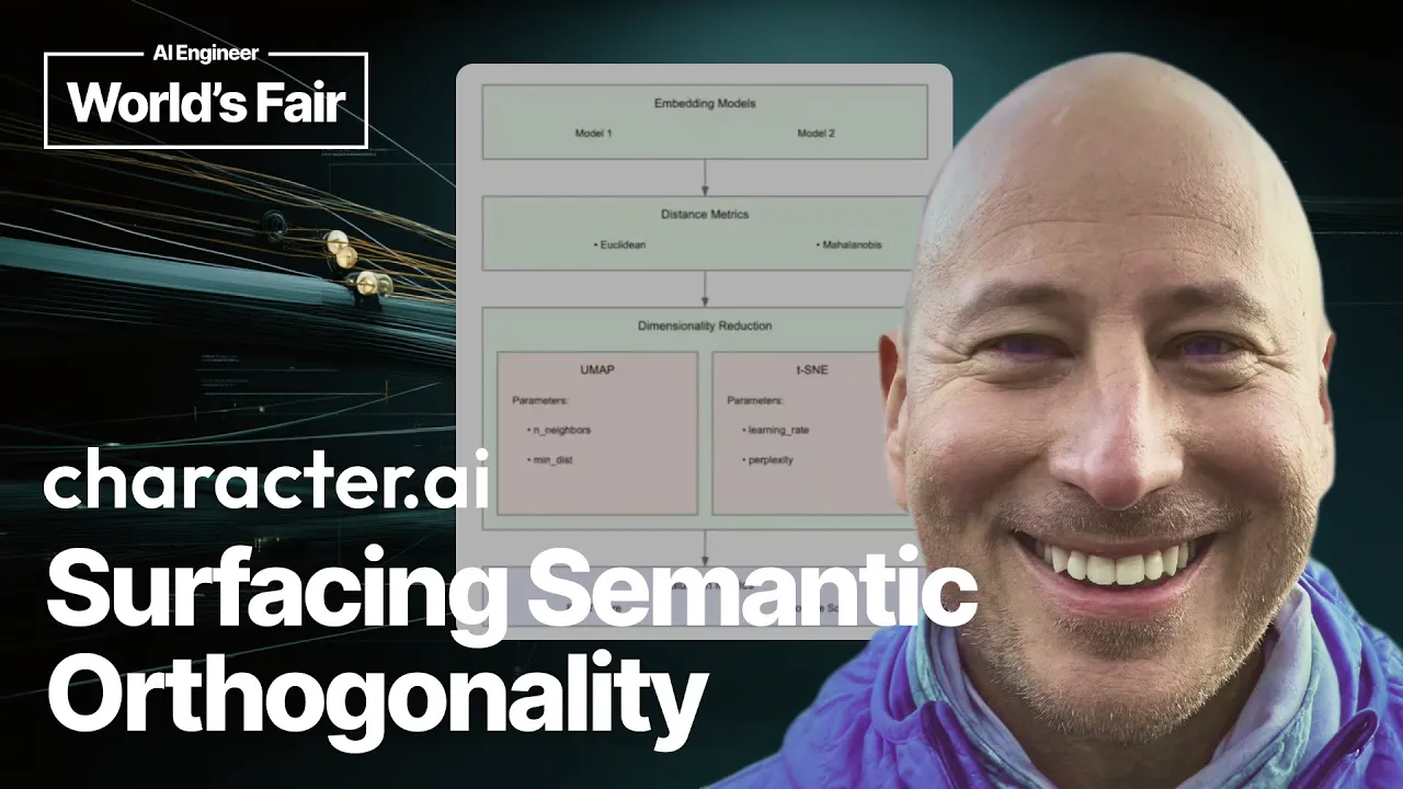
00:08:28.640 | So, uh, so after using an embedding model that was tested for, um, um, for best fit, we'll, we'll get
00:08:38.240 | into that in a second. Uh, there was, uh, a few different, uh, dimensionality reduction techniques
00:08:44.880 | that, that we looked at. And then, uh, each of those had hyperparameters and values for those
00:08:49.200 | hyperparameters in grid search. And then, uh, there's multiple distance metrics that could always be,
00:08:53.760 | be used, uh, in, in, in, in clustering. And so I'll get into that, uh, as well in this presentation
00:08:59.280 | and just doing a quick time check because I'm gonna have to, uh, go through this. I, anyways,
00:09:04.240 | so then, uh, with, um, uh, clusters, once the clusters were developed, uh, to an optimal, uh,
00:09:11.280 | separation by silhouette score, uh, then we took the, uh, the prompt values that were at each centroid
00:09:18.320 | that were at each edge. There's four edges. And, uh, this is again, all according to past research
00:09:23.120 | that's done this in the past, but this has just never been done in this capacity. Uh, and so then, uh,
00:09:29.680 | each of those prompts were then, uh, using, uh, inference to another LLM, multiple LLMs actually,
00:09:36.320 | to corroborate and find the category labeling, labeling behind that, that centroid. And then,
00:09:41.520 | uh, we ended up with, uh, what's gonna be on the next slide. We also identified more bias that,
00:09:47.040 | that could be seeping into that process, but this is the result, uh, the clustered results by,
00:09:52.960 | by benchmark. Uh, you can see each color here represents a benchmark that I was just talking about.
00:09:57.440 | Each of these benchmark benchmarks might've over-indexed, uh, on a different area, but again,
00:10:02.240 | this is using, uh, k-means clustering after you, we'll, we'll get into the, the process here and how
00:10:07.280 | I optimized, uh, by this is kind of an interesting method. Once everything is clustered in aggregate and,
00:10:14.960 | and, and after everything is, uh, appended into one dataset, uh, to see where these benchmarks,
00:10:22.320 | uh, over-index, you can see the, uh, each one of these dots here is a prompt. And, uh, the x and y
00:10:30.000 | axis here are just dimensions. When I say just dimensions, they're highly normalized from a
00:10:34.160 | high dimensional space, but you can think of these as semantic space. Uh, the closer they are together,
00:10:39.600 | the more, um, common they are, the further away, uh, the, the more breadth and, and semantic meaning and
00:10:46.240 | coverage, uh, is, is, is, uh, uh, highlighted. So again, the, the point of this, this paper was to
00:10:54.320 | show what's happened in the past, also show where people can research further and show, uh, what areas
00:11:00.240 | might, uh, have not had as much research as in terms of the breadth, uh, that, uh, they could have, um,
00:11:06.640 | and, and this is a great means to evaluate as well, uh, because this shows you, uh, what is inside of,
00:11:15.040 | of either, you know, an LLM benchmark or whatever you want to measure and, and it doesn't add those
00:11:20.080 | compounds of using blue and rouge scores. Um, again, the harm categories we, we found, uh, in this case,
00:11:26.080 | controlled substances, suicide and self-harm, guns, illegal weapons, criminal planning, confessions,
00:11:34.560 | hate, which actually included identity hate according to inference, and PII and privacy.
00:11:41.280 | Um, so the bulk of the paper gets into variants that are used to optimize for the distance here in the,
00:11:49.280 | in the clusters, and this process could be reused. It could be also, uh, refined, but the framework is,
00:11:55.760 | is where the paper, um, I think, uh, has, has, has made advances in, in terms of what the framework
00:12:02.880 | could be to optimize for any benchmarks that are around a similar topic in semantic space.
00:12:10.400 | So, um, just to clarify this, this slide, uh, used more than one embedding model, used more than
00:12:20.160 | one distance metric, used more than one means to have a dimensionality reduction, and then, uh,
00:12:26.400 | optimized for hyperparameters that were found by past research to be, uh, the most impactful,
00:12:31.440 | and then, uh, optimized for those values from those hyperparameters, which, you know, could have been a
00:12:37.520 | lot of compute, and then, um, more, ideally more than one evaluation metric. You can see a reference to
00:12:43.600 | BERT score at the bottom. Tried that. Uh, everything was ultimately optimized for silhouette score in order to
00:12:51.280 | optimize for the, the, the, the distance and the separation of each, each cluster. But BERT score,
00:12:57.200 | I thought, or the hypothesis was that BERT score would actually tell you in terms of tokens, uh, the
00:13:05.440 | difference between one cluster and the next. BERT score, the, the results actually came back like 1.0 for
00:13:10.000 | every cluster. And, uh, turns out BERT score is actually not the best metric to use because for, for,
00:13:15.760 | for, uh, data sets that have the same topic or a similar topic, like AI safety,
00:13:21.520 | or adversarial, uh, uh, data sets like, like, like, like AI safety data sets, um, where you fine tune a
00:13:28.320 | model based on what not to do. Um, uh, BERT score didn't, didn't, didn't work here. And so that the,
00:13:35.920 | the secondary metric used here was, uh, performance, performance time. So, so we optimized for the best
00:13:41.840 | silhouette score, and then of the best silhouette scores that were in the same confidence interval,
00:13:46.960 | uh, we're able to find that the most performant, uh, in terms of performance to scale.
00:13:51.120 | So, uh, sample size presumptions, um, this is, these are what went into the sample size calculation.
00:13:58.160 | Why are we doing this? Because the theory for, uh, why we want to do this is to, uh, query and look at
00:14:07.200 | the differences of, uh, over-indexing in a certain cluster from each benchmark. Um, you can see here,
00:14:12.880 | I hope you can see my screen where, where I'm highlighting, the maximum clusters we had to assume was
00:14:16.640 | 15. Um, obviously we didn't get 15, but going into it, uh, we had to presume that because the,
00:14:23.920 | the most recent paper had a taxonomy listing, uh, between 12 and 13, adding 10 percent to that,
00:14:29.520 | according to past research, because we, we would have had, uh, in theory, more, uh, clusters, um,
00:14:35.760 | or at least more semantic space covered by looking at more than one dataset. So, um, we had to presume
00:14:41.520 | something, and so that was rationale to presume 15. Uh, significance level, because it was 15 clusters,
00:14:48.160 | and we wanted to look at this by each benchmark, 15 split, you know, five split by 15. Uh, the
00:14:55.200 | significance level, to be safe, dropped to 0.15. Um, and the effect size is large because, uh, according
00:15:04.800 | to past research, there's been, uh, a citation here in the paper that stated that it wouldn't matter
00:15:12.320 | the results that we'd find in terms of a benchmark having a slightly different, uh, over indexing for,
00:15:17.680 | uh, each harm category. It wouldn't matter unless effect size is 0.5 at least. So I thought, okay,
00:15:22.960 | that's fine. That's rationale to, to use a high effect size here. Um, um, didn't know what we'd get,
00:15:28.960 | uh, because this, this was never really done in this capacity in terms of prompts. Uh, anyways,
00:15:36.080 | with this calculation, uh, ended up with a minimum required sample size per benchmark of 1,635,
00:15:42.400 | and with a total sample size across all benchmarks of 8,175. Uh, outlier removal, uh, did this again
00:15:50.080 | for the whole entire dataset, uh, used compared IQR method and z-score method. Uh, counterintuitively,
00:15:55.760 | the z-score method actually, uh, was looser and allowed for actually more prompts here, uh,
00:16:01.040 | that, you know, could be considered an outlier if we're using our IQR method. What was interesting
00:16:05.920 | was because this is so right skewed, uh, this is not a normal distribution. This is extremely right skewed,
00:16:12.000 | uh, in terms of prompt length. Uh, the z-score actually looked at the standard deviation as it does
00:16:20.000 | and removed less because the standard deviation was so large here. So not only are there long
00:16:25.440 | prompts, there's just a lot of standard deviation amongst those long, long prompts, which was great
00:16:30.640 | because the, these prompts here turned out to be, uh, relatively valuable and showing up in, in a
00:16:36.080 | semantic space that, that it was kind of of its own. So that said, um, this, this, this worked, uh, in terms
00:16:42.960 | of the, the result, uh, still right skewed, but, uh, better if you, especially with the magnitude, uh, down
00:16:49.680 | there, uh, uh, quite a bit better, uh, but still right skewed, uh, there's gonna be the next three
00:16:57.040 | slides. I'm gonna talk about the variance and then I'm gonna talk about the results. Um, so the variance,
00:17:03.520 | uh, again, that I iterated through, uh, the, um, embedding models, uh, there had to be some rationale
00:17:11.840 | there, uh, in terms of what embedding model to use. Uh, mini LM is something that we, uh, started using
00:17:19.680 | because of its scalability. Uh, it produces high quality embedding values for each, each prompt.
00:17:25.920 | For those of you that are unfamiliar, um, it's, uh, it'll just take a prompt and assign a semantic,
00:17:32.240 | uh, vectorized, very high dimensional, uh, value. It's a mini, mini LM, not only does a high quality
00:17:40.000 | embedding value, but also, uh, performs some reduction of, of, of dimensions. And I'll get
00:17:45.600 | into why we even go, go through the, the hassle of, uh, reducing, uh, dimensionality on the next,
00:17:51.360 | the next step. But then there's also an efficient memory usage. It's, it's really small and it's,
00:17:55.440 | it's, uh, been used in a lot of research, uh, especially of the same kind for, for looking at prompts
00:18:00.080 | and semantic space. MP net gets into using more memory. It excels at contextual and sequential
00:18:05.600 | encoding, uh, higher memory usage. So it's the next step up, even though they're both small and
00:18:10.480 | comparable. I wanted to see the direction it would go. Um, both are 512 tokens. This isn't on the paper,
00:18:16.240 | so I added a note down below just to clarify for those of you listening, um, that, uh, there's,
00:18:21.920 | there's memory differences and they're relatively substantial. It's one difference. So we wanted to see
00:18:27.680 | if there was a difference at all and, and using these, um, embedding models as they became more
00:18:32.480 | sophisticated, um, for reducing dimensionality further, which is important to do with, uh, there's,
00:18:40.560 | there's some research that suggests, um, even though we lose more information, uh, we still, uh, in order
00:18:48.320 | to cluster, uh, need something here, uh, to allow us to have manageable values that we're clustering on.
00:18:57.040 | So TSNE, uh, preserves local structure but struggles with global relationships that actually, in this case,
00:19:04.080 | could be useful. UMAP, uh, preserves both local and global structure while scaling efficiently. Different
00:19:11.600 | hyperparameters for each. Uh, for TSNE, we had to draw on past research, um, so prioritize perplexity and
00:19:19.520 | learning rate. For UMAP, uh, again, had to draw upon past research that was most impactful for, for a
00:19:24.640 | similar use case and looked at n-neighbors and, and min-dist. The, uh, Euclidean distance is something that
00:19:31.360 | is kind of a common, uh, default to use. Uh, works well in low dimensional spaces, doesn't work well when you get into
00:19:39.120 | high dimensions, uh, because the differences are, are, are too profound. Um, so Mahalanobis is something
00:19:46.320 | else that we looked at to compare. It incorporates an, an inverse, uh, covariance matrix, uh, to account for
00:19:54.000 | dimensional correlations. And I was really excited about the Mahalanobis distance. The research in the
00:20:02.000 | past suggests that it could be one of the best metrics to look at because it accounts for dimensional
00:20:06.400 | correlations, which you would presume would be extremely interesting. Um, it didn't, uh, in the
00:20:12.560 | results, we're looking at the top eight out of 16 different combinations here. Uh, there's 16. You think
00:20:17.760 | there might have been more, but, uh, the, uh, for grid search, I had to, uh, whittle, uh, some of the values
00:20:25.440 | down in order to, uh, uh, have this performance. And, uh, if you look at the top eight of the, the cluster optimization results,
00:20:33.680 | again, by, uh, silhouette score, you can see that there's some overlap visually in the confidence interval.
00:20:38.880 | And among that overlap, you see the second one from the top, um, mini LM, Euclidean, uh, UMAP, uh, uh,
00:20:47.520 | the end of the 30 min dist is 0.1. So, um, this is also, you could look at the efficiency, which is
00:20:55.280 | normal and normalized, uh, in terms of, uh, seconds in terms of time processing time. And this makes more
00:21:01.360 | sense to scale. If everything's in the same comfort or within the same confidence range. Um, so, uh, number
00:21:08.160 | of clustered clusters was reviewed for diligence, um, because that was important because also counterintuitive,
00:21:15.600 | we expected more because the taxonomies were getting large. There's a lot more semantic space,
00:21:21.040 | a lot more harms that were covered. It was counterintuitive to get, uh, six.
00:21:24.880 | Uh, elbow method actually suggests between five and six. Silhouette analysis suggested six. Uh, there's
00:21:33.840 | research that suggests that if you're between two values to use the one that makes the most sense to you.
00:21:38.560 | So we use six. Um, this influenced prompt values and centroids, um, excuse me, the, the inference, uh,
00:21:46.640 | uh, that, that we gave to the, the, the prompt values, uh, at the centroids, uh, were influenced by,
00:21:54.000 | um, LLMs, but they didn't, there was not much variance here at all. Uh, there might have been a plural
00:21:59.040 | word, uh, versus a singular word if you move across, uh, model families and into the next model family for
00:22:05.920 | inference. So this is, these are the, the, uh, the, the clusters that developed from, from these
00:22:10.560 | benchmarks and insights here, I'm getting down to the end of this, uh, talk and then I'm going to be
00:22:16.560 | opening up for questions, but I want to emphasize, uh, the insights and then what we learned here in the
00:22:21.120 | insights, if you know, the sparsity and variant breadth, like I, uh, mentioned before, um, the hate and
00:22:27.120 | identity hate category, it's very focused, uh, it could be more, more, but then actually there's a,
00:22:33.360 | there's a, a tangent there on, uh, uh, the inability for, uh, LLMs to capture hate speech right now,
00:22:42.240 | currently, uh, and that's a criticism of a lot of, uh, AI tools, uh, it should be better, right? Well,
00:22:48.480 | this is because we don't have as much ground truth and this, this, this highlights that. Also, uh, there is
00:22:53.840 | anthropomorphism that is happening quite often and a lot of other harms that are happening
00:22:58.400 | psychologically to people using AI that, that are not, uh, evident here. Um, it's not that they're
00:23:04.000 | debated, they're, they're, they're harms, they're just not, not explored. So this allows you to pivot
00:23:10.080 | and go, okay, these are harms that we looked at in the past. What else can we look at in order to,
00:23:14.320 | I don't want to be fear-mongering, um, but there are, like I said in the beginning of the talk,
00:23:20.960 | uh, there are, uh, harms that will happen from AI use. Uh, one, exacerbation of suicide and self-harm.
00:23:30.160 | In other words, if someone's using an AI tool and they're thinking about self-harm and suicide,
00:23:35.520 | it could exacerbate that, um, through, uh, sycopency. And I think we all know, are aware of that, um, uh,
00:23:44.240 | but some people are not, and some people are, um, possibly, uh, more susceptible to this than others.
00:23:51.120 | So, so, uh, there's always going to be some harms with, with usage, not that AI is causing those per
00:23:57.440 | se, it's the usage. And so, uh, this is something that, um, we thought was interesting. In terms of
00:24:02.800 | looking at the bias in clusters, there's still the bias in clusters that exist. If you look at the prompt,
00:24:06.240 | the distribution of prompt links by benchmark, different, uh, and that's all I'm going to say
00:24:10.080 | about that, um, because we're almost out of time when I talk about the limitations and then the, uh,
00:24:14.960 | takeaways. Limitations, obviously there's, there's, uh, methodological, methodological limitations here,
00:24:20.480 | uh, could have increased the sample size, for example, uh, dimensionality reduction loses information.
00:24:26.400 | There's bias actually inherent in the embeddings models that we're trying to get out.
00:24:29.360 | Uh, um, choosing the benchmarks, this is only five. I mean, I generalize because there's a lot of private
00:24:34.640 | benchmarks. Um, equal benchmark weighting presumes that people are using this equally
00:24:40.000 | they may not, uh, human biases that are inherent in research, implicit Western views in our research,
00:24:45.360 | um, in terms of the past harm as well. And, uh, the author's technical backgrounds, including myself,
00:24:52.320 | uh, um, because of the technical background, we might not have been thinking about harms that are
00:24:57.440 | actually, um, something that might be more of a priority that, that we might not have seen, not have
00:25:02.000 | seen, uh, future research directions, um, could include harm benchmarks for more, more cultural contexts.
00:25:08.480 | Um, there could be more exploration of prompt response relationships, because this is only
00:25:12.720 | looking at the prompts intended to look at the prompts, prompt response relationships,
00:25:16.560 | but ran out of time and space in the paper. And then, um, if you were to apply this methodology
00:25:22.400 | framework to domain specific data sets, um, and investigate differences this way, this, this is a,
00:25:28.000 | an evaluation method that is, uh, uh, uh, solid because it shows you what, what, what's in the data.
00:25:35.360 | Top four conclusions, last slide. Uh, there are six primary harm categories that we identified
00:25:42.160 | with varying coverage and breadth from each benchmark. Uh, semantic coverage gaps, as you've seen,
00:25:47.280 | exist across recent benchmarks and will over time as we change the definition for harms. Uh, the third,
00:25:53.440 | uh, was that we've found optimal clustering configuration framework for this particular use
00:25:58.640 | case. And, um, this could be scaled for, for use in other benchmarks of similar topical use or, uh,
00:26:05.680 | other LLM applications of other similar, similar topical use. Uh, again, it shows you amongst a collection of
00:26:13.040 | things of similar topics, how something might over index and under index fourth, uh, plotting semantic
00:26:19.760 | space. Um, again, this is a, uh, transparent evaluation approach that, uh, allows for more action and more
00:26:25.360 | insight than the stereotypical region blue scores, which are binomial, uh, related to precision and recall
00:26:31.840 | that we're biased on using. So this allows you to, to have more insights. Thank you very much. Uh, we're