Lesson 6: Deep Learning 2019 - Regularization; Convolutions; Data ethics

00:00:00.000 | All right, welcome to lesson six where we're going to do a deep dive into computer vision,

00:00:09.820 | convolutional neural networks, what is a convolution, and we're also going to learn the final regularization

00:00:18.040 | tricks after last lesson learning about weight decay and slash L2 regularization.

00:00:27.520 | I want to start by showing you something that I'm really excited about and I've had a small hand in helping to create.

00:00:35.960 | For those of you that saw my talk on TED.com, you might have noticed this really interesting demo that we did about four

00:00:44.440 | years ago showing a way to quickly build models with unlabeled data.

00:00:52.160 | It's been four years, but we're finally at a point where we're ready to put this out in the world and let people use it.

00:00:59.000 | And the first people we're going to let use it are you folks.

00:01:04.160 | So the company is called platform.

00:01:06.080 | I and the reason I'm mentioning it here is that it's going to let you create models on different types of data sets to what you can do now.

00:01:14.520 | That is to say data sets that you don't have labels for yet.

00:01:18.400 | We're actually going to help you label them.

00:01:20.760 | So this is the first time.

00:01:23.720 | This has been shown before.

00:01:28.120 | So I'm pretty thrilled about it.

00:01:33.000 | And let me give you a quick demo when you so if you go to platform.

00:01:39.560 | I and choose get started.

00:01:44.280 | You'll be able to create a new project and if you create a new project,

00:01:48.240 | you can either upload your own images.

00:01:52.240 | Uploading at 500 or so works pretty well.

00:01:55.400 | You can upload a few thousand,

00:01:57.040 | but to start upload 500 or so they all have to be in a single folder.

00:02:03.600 | And so we're assuming that you've got a whole bunch of images that you haven't got any labels for.

00:02:07.680 | Or you can start with one of the existing collections if you want to play around.

00:02:11.080 | So I've started with the cars collection kind of going back to what we did four years ago.

00:02:17.640 | And so this is what happens when you first.

00:02:21.840 | Go into platform AI and look at the collection of images you uploaded a random sample of them will appear on the screen.

00:02:29.840 | And as you'll recognize probably they are projected.

00:02:34.920 | From a deep learning space into a 2D space using a pre-trained model.

00:02:41.000 | And for this initial version, it's an image net model we're using as things move along will be adding more and more pre-trained models.

00:02:49.720 | And what I'm going to do is I want to add labels to this data set representing which angle a photo of the car was taken from,

00:02:58.200 | which is something that actually image that's going to be really bad at isn't it?

00:03:03.080 | Because image net has learned to recognize the difference between cars versus bicycles and image net knows that the angle you take a photo on actually doesn't matter.

00:03:13.400 | So we want to try and create labels using the kind of thing that actually image net specifically learn to ignore.

00:03:20.560 | So the projection that you see we can click these layer buttons at the top to switch to user projection using a different layer of the neural net.

00:03:31.440 | Right and so here's the last layer which is going to be a total waste of time for us because it's really going to be projecting things based on what kind of thing it thinks it is.

00:03:41.760 | And the first player is probably going to be a waste of time for us as well because there's very little interesting semantic content there.

00:03:49.040 | But if I go into the middle in layer three, we may well be able to find some some some differences there.

00:03:56.240 | So then what you can do is you can click on the projection button here and you can actually just press up and down rather than just pressing the other arrows at the top to switch between projections or left and right switch between layers.

00:04:08.840 | And what you can do is you can basically look around until you notice that there's a projection which is kind of separated out things you're interested in.

00:04:18.040 | And so this one actually I notice that it's got a whole bunch of cars that are kind of from the top front front right over here.

00:04:34.600 | OK, so if we zoom in a little bit, we can double check because like, yeah, that looks pretty good.

00:04:39.560 | They're all kind of front right. So we can click on here to go to selection mode and we can kind of grab a few.

00:04:46.800 | And then you should check. And so what we're doing here is we're trying to take advantage of the combination of human plus machine.

00:04:53.200 | The machine is pretty good at quickly doing calculations, but as a human, I'm pretty good at looking at a lot of things at once and seeing the odd one out.

00:05:01.800 | So in this case, I'm looking for cars that aren't front right. And so by laying them all in front of me, I can do that really quickly.

00:05:07.320 | It's like, OK, definitely that one. So just click on the ones that you don't want.

00:05:13.640 | All right, so good. So then you can just go back. And so then what you can do is you can either put them into a new category by typing create new label or you can click on one of the existing ones.

00:05:23.640 | So before I came, I just created a few. So here's front right. So I just click on it here.

00:05:29.120 | There we go. OK, and so that's the basic idea is that you kind of keep flicking through different layers or projections to try and find groups that represent the things you're interested in.

00:05:39.520 | And then over time, you'll start to realize that there are some things that are a little bit harder.

00:05:45.240 | So, for example, I'm having trouble finding sides. So what I can do is I can see over here, there's a few sides.

00:05:51.840 | So I can zoom in here and click on a couple of them like this one and this one.

00:06:00.880 | That one. OK, I mean, I'll say find similar.

00:06:06.840 | And so this is going to basically look in that that projection space and not just at the images that are currently displayed,

00:06:14.680 | but all of the images that you uploaded. And hopefully I might be able to label now a few more side images at that point.

00:06:22.800 | So it's going through and checking all of the images that you uploaded to see if any of them have projections in this space which are similar to the ones I've selected.

00:06:35.760 | And hopefully we'll find a few more of what I'm interested in.

00:06:43.280 | OK, so now if I want to try to find a projection that separates the sides from the front right, I can click on each of those two.

00:06:52.440 | And then over here, this button is now called switch to the projection that maximizes the distance between the labels.

00:06:57.840 | So now what this is going to do is try and find the best projection that separates out those classes.

00:07:03.560 | And so the goal here is to help me visually inspect and quickly find a bunch of things that I can use to label.

00:07:13.800 | So like they're the kind of the key features and it's done a good job.

00:07:18.200 | You can see down here, we've now got a whole bunch of sides which I can now grab because I was having a lot of trouble finding them before.

00:07:26.120 | And it's always worth double checking.

00:07:31.760 | And it's kind of interesting to see how the neural nets behave like there seems to be more sports cars in this group than average as well.

00:07:38.440 | So it's kind of found side angles of sports cars. So that's kind of interesting.

00:07:42.720 | So then I can click. All right. So I've got those. So now I'll click side and there we go.

00:07:47.920 | So once you've done that a few times, I find if you've got, you know, a hundred or so labels, you can then click on the train model button and it'll take a couple of minutes and come back and show you your train model.

00:08:01.720 | And after it's trained, which I did it on a smaller number of labels earlier, you can then switch this very opacity button and it'll actually kind of fade out the ones that are already predicted pretty well.

00:08:14.120 | And it'll also give you an estimate as to how accurate it thinks the model is.

00:08:19.240 | The main reason I mentioned this for you is that so that you can now click the download button and it'll download the predictions.

00:08:26.640 | Which is what we hope will be interesting to most people. But what I think will be interesting to you as deep learning students is it will download your labels.

00:08:33.640 | So now you can use that labeled subset of data along with the unlabeled set that you haven't labeled yet to see if you can, you know, see if you can build a better model and platform AI is done for you.

00:08:47.160 | See if you can use that initial set of data to kind of get going, creating models of stuff which you weren't able to label before.

00:08:55.400 | Clearly, there are some things that this system is better than others for things that require.

00:09:02.040 | You know, really zooming in closely and taking a very, very close inspection.

00:09:06.440 | This isn't going to work very well. This is really designed for things that the human eye can kind of pick up fairly readily.

00:09:12.880 | But we'd love to get feedback as well, and you can click on the help button to get feedback and give feedback.

00:09:19.240 | And also, there's a platform AI discussion topic in our forum. So, Arshak, if you can stand up, Arshak's the CEO of the company.

00:09:27.840 | He'll be there helping out answering questions and so forth.

00:09:33.440 | So, yeah, I hope people find that useful. It's been many years getting to this point and I'm glad we're finally there.

00:09:47.480 | OK, so one of the reasons I wanted to mention this today is that we're going to be doing a big dive into convolutions later in this lesson.

00:09:56.160 | So I'm going to circle back to this to try and explain a little bit more about how that is working under the hood and give you a kind of a sense of what's what's going on.

00:10:04.160 | But before we do, we have to finish off last week's discussion of regularization.

00:10:10.280 | And so we were talking about regularization specifically in the context of the Tabular Learner because the Tabular Learner, this was the forward method.

00:10:19.600 | Sorry, this is the init method in the Tabular Learner. And our goal was to understand everything here.

00:10:26.920 | And we're not quite there yet. Last week, we were looking at the adult dataset, which is a really simple kind of oversimple dataset that's just for toy purposes.

00:10:38.440 | So this week, let's look at a dataset that's much more interesting, a Kaggle competition dataset.

00:10:43.040 | So we know kind of what the best in the world and Kaggle competition results tend to be much harder to beat than academics data.

00:10:51.880 | The art results tend to be because a lot more people work on Kaggle competitions than most academic datasets.

00:10:57.320 | So it's a really good challenge to try and do well on a Kaggle competition dataset.

00:11:01.880 | So this one, the Rossman dataset, they've got 3000 drugstores in Europe and you're trying to predict how many products they're going to sell in the next couple of weeks.

00:11:15.720 | So one of the interesting things about this is that the test set for this is from a time period that is more recent than the training set.

00:11:25.600 | And this is really common, right? If you want to predict things, there's no point predicting things that are in the middle of your training set.

00:11:30.480 | You want to predict things in the future.

00:11:34.440 | Another interesting thing about it is the evaluation metric they provided is the root mean squared percent error.

00:11:40.640 | So this is just a normal root mean squared error, except we go actual minus prediction divided by actual.

00:11:46.360 | So in other words, it's the percent error that we're taking the root mean squared of.

00:11:52.000 | So there's a couple of interesting features, always interesting to look at the leaderboard.

00:11:56.400 | So the leaderboard, the winner, was 0.1.

00:12:00.760 | The paper that we've roughly replicated was 0.105, 0.106, and tenth place out of 3000 was 0.11-ish, a bit less.

00:12:16.480 | All right. So we're going to skip over a little bit,

00:12:23.360 | which is that the data that was provided here was they provided a small number of files,

00:12:30.480 | but they also let competitors provide additional external data as long as they shared it with all the competitors.

00:12:37.840 | And so in practice, the data set we're going to use contains, I can't remember, six or seven tables.

00:12:44.520 | The way that you join tables and stuff isn't really part of a deep learning course, so I'm going to skip over it.

00:12:50.560 | And instead, I'm going to refer you to introduction to machine learning for coders,

00:12:54.280 | which will take you step by step through the data preparation for this.

00:12:58.960 | We've provided it for you in Rossman Data Clean, so you'll see the whole process there.

00:13:10.720 | And so you'll need to run through that notebook to create these pickle files that we read here.

00:13:17.600 | Can you see this in the back? OK, great.

00:13:22.840 | I just want to mention one particularly interesting part of the Rossman Data Clean notebook,

00:13:29.280 | which is you'll see there's something that says add date part, and I wanted to explain what's going on here.

00:13:34.520 | I've been mentioning for a while that we're going to look at time series,

00:13:38.000 | and pretty much everybody who I've spoken to about it has assumed that I'm going to do some kind of recurrent neural network.

00:13:43.600 | But I'm not. Interestingly, the kind of the main academic group that studies time series is econometrics.

00:13:51.360 | And but they tend to study one very specific kind of time series,

00:13:54.800 | which is where the only data you have is a sequence of time points of one thing.

00:14:00.800 | Like, that's the only thing you have is one sequence. In real life, that's almost never the case.

00:14:05.720 | Normally, you know, if we would have some information about the store that that represents or the people that it represents,

00:14:11.480 | we'd have metadata, we'd have sequences of other things measured at similar time periods or different time periods.

00:14:19.320 | And so most of the time I find in practice, the state of the art results when it comes to competitions on kind of more real world datasets,

00:14:29.440 | don't tend to use recurrent neural networks, but instead they tend to take the time piece,

00:14:35.000 | which in this case it was a date we were given in the data, and they add a whole bunch of metadata.

00:14:41.440 | So in our case, for example, we've added day of week. So we were given a date, right?

00:14:46.360 | We've had a day of week, year, month, week of year, day of month, day of week, day of year,

00:14:55.320 | and then a bunch of bullions. Is it the month start or end? Quarter, year, start or end?

00:14:59.080 | Elapsed time since 1970, so forth. If you run this one function, add date part and pass it a date,

00:15:06.840 | it'll add all of these columns to your dataset for you.

00:15:10.240 | And so what that means is that let's take a very reasonable example.

00:15:15.720 | Purchasing behavior probably changes on payday. Payday might be the fifteenth of the month.

00:15:21.040 | So if you have a thing here called this is day of month here, right,

00:15:25.240 | then it'll be able to recognize every time something is a 15 there and associated it with a higher,

00:15:31.920 | in this case, embedding matrix value. So this way, basically, you know,

00:15:39.280 | we can't expect a neural net to do all of our feature engineering for us.

00:15:43.080 | We can expect it to kind of find non-linearities and interactions and stuff like that.

00:15:47.080 | But for something like taking a date like this and figuring out that the fifteenth of the month

00:15:54.360 | is something when interesting thing happen, it's much better if we can provide that information for it.

00:16:00.000 | So this is a really useful function to use. And once you've done this,

00:16:03.920 | you can treat many kinds of time series problems as regular tabular problems.

00:16:09.240 | I say many kinds, not all. You know, if there's very complex kind of state involved in a time series,

00:16:15.640 | such as, you know, equity trading or something like that, this probably won't be the case,

00:16:20.080 | or this won't be the only thing you need. But in this case, it'll get us a really good result.

00:16:27.680 | And it's in practice most of the time. I find this works well.

00:16:31.880 | Tabular data is normally in pandas. So we just stored them as standard Python pickle files.

00:16:37.200 | We can read them in. We can take a look at the first five records.

00:16:41.400 | And so the key thing here is that we're trying to, on a particular date, for a particular store ID,

00:16:47.720 | we want to predict the number of sales. Sales is the dependent variable.

00:16:54.440 | So the first thing I'm going to show you is something called preprocessors.

00:16:58.720 | You've already learned about transforms. Transforms are bits of code that run every time something is grabbed from a data set.

00:17:06.520 | And so it's really good for data augmentation that we'll learn about today,

00:17:10.200 | which is that it's going to get a different random value every time it's sampled.

00:17:14.280 | Preprocessors are like transforms, but they're a little bit different,

00:17:19.360 | which is that they run once before you do any training.

00:17:23.520 | And really importantly, they run once on the training set.

00:17:29.160 | And then any kind of state or metadata that's created is then shared with the validation and test set.

00:17:35.920 | Let me give you an example. When we've been doing image recognition and we've had a set of classes for like all the different pet breeds,

00:17:43.760 | and they've been turned into numbers,

00:17:46.120 | the thing that's actually doing that for us is a preprocessor that's being created in the background.

00:17:50.520 | So that makes sure that the classes for the training set are the same as the classes for the validation and the classes of the test set.

00:17:57.760 | So we're going to do something very similar here. For example, if we create a little small subset of the data for playing with,

00:18:05.280 | this is a really good idea when you start with a new data set.

00:18:08.120 | So I've just grabbed 2000 IDs at random. And then I'm just going to grab a little training set and a little test set,

00:18:16.440 | half and half of those 2000 IDs. I'm just going to grab five columns and then we can just play around with this nice and easy.

00:18:23.600 | So here's the first few of those from the training set.

00:18:27.600 | As you can see, one of them is called promo interval and it has these strings.

00:18:33.080 | And sometimes it's missing. In pandas, missing is NIN.

00:18:38.000 | So the first preprocessor I'll show you is categorify and categorify does basically the same thing that that classes thing for image recognition does for our dependent variable.

00:18:50.320 | It's going to take these strings. It's going to find all of the possible unique values of it and it's going to create a list of them and then it's going to turn the strings into numbers.

00:18:59.840 | So if I call it on my training set that will create categories there and then I call it on my test set passing in test equals true that makes sure it's going to use the same categories that I had before.

00:19:12.400 | And now when I say dot head, it looks exactly the same and that's because pandas has turned this into a categorical variable,

00:19:20.440 | which internally is storing numbers that externally is showing me the strings, but I can look inside promo interval to look at the cat categories.

00:19:31.120 | This is all standard pandas here to show me a list of all of the what we would call classes in fast AI or would be called categories in pandas.

00:19:42.480 | And so then if I look at the cat codes, you can see here this list here is the numbers that are actually stored minus one minus one one minus one one right.

00:19:52.960 | One by one of these minus ones.

00:19:56.080 | The minus ones represent and I am they represent missing so pandas uses a special code minus one to be mean missing now as you know these are going to end up in an embedding matrix.

00:20:08.920 | And we can't look up item minus one embedding matrix so internally in fast AI we add one to all of these.

00:20:18.640 | Another useful preprocessor is fixed missing and so again you can call it on the data frame you can call on the test passing in test equals true and this will create for everything that's missing anything that has a missing value.

00:20:33.160 | It will create an additional column with the column name underscore NA so competition distance underscore NA and it'll set it for true for any time that was missing.

00:20:44.160 | And then what we do is we replace competition distance with the median for those why do we do this well because very commonly the fact that something's missing.

00:20:55.640 | Is of itself interesting like it turns out the fact that this is missing helps you predict your outcome right so we certainly want to keep that information in a convenient Boolean column so that our deep learning model can use it to predict things.

00:21:10.160 | But then we need competition distance to be a continuous variable so we can use it in the continuous variable part of our model so we can replace it with almost any number right because if it turns out that the missing this is important.

00:21:22.640 | They can use the interaction of competition distance NA and competition distance to make predictions so that's what fixed missing does.

00:21:31.520 | You don't have to manually call preprocessors yourself when you call.

00:21:41.480 | Any kind of item list creating creator you can pass in a list of preprocessors which you can create like this.

00:21:49.720 | OK so this is saying OK want to feel missing I want to categorify I want to normalize so for continuous variables it'll subtract the mean and divide by the standard deviation to help a train more easily and so you just say those are my procs and then you can just pass it in there and that's it and later on you can go data export and it'll save all the better data for that data bunch so you can later on loaded in.

00:22:13.280 | Knowing exactly what your category codes are exactly what median values use from replacing the missing values and exactly what means and standard deviations you normalize by.

00:22:25.440 | OK so the main thing you have to do if you want to create a data bunch of tabular data is find out or tell it what are your categorical variables and what are your continuous variables.

00:22:37.680 | And as we discussed last week briefly your categorical variables are not just strings and things but also I include things like.

00:22:47.840 | Day of week and month and day of month even though their numbers I make them categorical variables because for example day of month I don't think it's going to have a nice smooth curve I think that the 15th of the month and the 1st of the month and the 30th of the month are probably going to have different

00:23:06.720 | purchasing behavior to other days of the month and so therefore if I make it a categorical variable it's going to end up creating an embedding matrix and those different days of the month can get different behaviors.

00:23:19.440 | So you've actually got to think carefully about which things should be categorical variables and on the whole if in doubt and there are not too many levels in your category that's called the cardinality if your cardinality is not too high I would put it as a categorical variable.

00:23:35.200 | You can always try in each and see which works best.

00:23:38.880 | So our final data frame that we're going to pass in is going to be our training set with the categorical variables and the continuous variables and the dependent variable and the date.

00:23:49.120 | And the date we're just going to use to create a validation set where we're basically going to say the validation set is going to be the same number of records at the end of the time period that the test set is for Kaggle and so that way we should be able to validate our model nicely.

00:24:06.080 | OK so now we can create a tabular list so this is our standard data block API that you've seen a few times from a data frame passing all of that information split it into valid versus train label it with a dependent variable.

00:24:22.040 | And here's something I don't think you've seen before.

00:24:25.320 | Label class.

00:24:27.560 | This is our dependent variable and as you can see this is this is sales it's not a float.

00:24:34.320 | It's an in 64 if this was a float then fast AI would automatically know or guess that you want to do a regression.

00:24:43.120 | But this is not a float.

00:24:44.560 | It's an int so fast I was going to assume you want to do a classification.

00:24:48.400 | So when we label it we have to tell it that the class of the labels we want is a list of floats not a list of categories which would otherwise be the default.

00:24:58.840 | So this is the thing that's going to automatically turn this into a regression problem for us.

00:25:04.280 | And then we create a data bunch.

00:25:05.680 | So I wanted to remind you again about doc which is how we find out more information about this stuff in this case all of the labeling functions in the data blocks API will pass on any keywords they don't recognize to the label class.

00:25:24.560 | So one of the things I've passed in here is log and so that's actually going to end up in float list and so if I go doc float list I can see a summary.

00:25:33.400 | And I can even jump into the full documentation and it shows me here that log is something which if true it's going to take the logarithm of my dependent variable.

00:25:44.640 | Why am I doing that so this is the thing that's actually going to automatically take the log of my way.

00:25:50.680 | The reason I'm doing that is because as I mentioned before the evaluation metric is root mean squared percentage error.

00:26:00.760 | And first I know pi torch has a root mean squared percentage error loss function built in.

00:26:10.320 | I don't even know if such a loss function would work super well but if you want to spend the time thinking about it you'll notice that this ratio if you first take the log of y and y hat then becomes a difference rather than the ratio.

00:26:25.320 | So in other words if you take the log of y then this becomes root mean squared error so that's what we're going to do.

00:26:33.160 | We're going to take the log of y and then we're just going to use root mean squared error which is the default for aggression problem so we won't even have to mention it.

00:26:42.840 | The reason that we have this year is because this is so common right basically anytime you're trying to predict something that's like a population or a dollar amount of sales.

00:26:54.560 | These kind of things tend to have long tail distributions where you care more about percentage differences and exact differences absolute differences.

00:27:03.880 | So you're very much very likely to want to do things with log equals true and to measure the root mean squared percent error.

00:27:13.360 | We've learned about the y range before which is going to use that sigmoid to help us get in the right range because this time the y values are going to be taken the

00:27:24.480 | log of it first we need to make sure that the y range we want is also the log so I'm going to take the maximum of the sales column.

00:27:33.040 | I'm going to multiply it by a little bit so that because remember how we said it's nice if your range is a bit wider than the range of the data and then we're going to take the log and that's going to be our maximum.

00:27:44.680 | So then our y range will be from zero to a bit more than the maximum.

00:27:51.840 | So now we've got our data bunch we can create a tabular learner from it and then we have to pass in our architecture and as we briefly discussed.

00:28:01.560 | For a tabular model architecture is literally the most basic fully connected network just like we showed in this picture.

00:28:12.200 | It's an input matrix multiply nonlinearity matrix multiply nonlinearity matrix multiply nonlinearity done.

00:28:23.320 | One of the interesting things about this is that this competition is three years old but I'm not aware of any significant advances at least in terms of architecture that would cause me to choose something different to what the third place folks did three years ago.

00:28:40.720 | We're still basically using simple fully connected models for this problem.

00:28:46.880 | Now the intermediate weight matrix is going to have to go from a 1000 activation input to a 500 activation output which means it's going to have to be 500000 elements in that weight matrix.

00:29:05.200 | That's an awful lot for a data set with only a few hundred thousand rows.

00:29:09.960 | So this is going to over fit and we need to make sure it doesn't.

00:29:14.000 | So one way to make sure it does well the way to make sure it doesn't is to use regularization.

00:29:19.560 | Not to reduce the number of parameters to use regularization.

00:29:23.800 | So one way to do that will be to use weight decay which fast AI will use automatically and you can vary it to something other than the default if you wish it turns out in this case we're going to want more regularization.

00:29:36.680 | And so we're going to pass in something called keys.

00:29:40.280 | This is going to provide dropout and also this one here and drop this is going to provide embedding dropout.

00:29:47.320 | So let's learn about what is dropout but the short version is dropout is a kind of regularization.

00:29:54.720 | This is the dropout paper.

00:29:59.000 | Nitish. How do you say this Srivastava it was Srivastava's master's thesis under Jeffrey Hinton and this picture from the original paper is a really good picture of what's going on.

00:30:15.640 | This first picture is a picture of a standard fully connected network.

00:30:19.360 | It's a picture of this and what each line shows is a multiplication of an activation times a weight.

00:30:28.760 | And then when you've got multiple arrows coming in that represents a sum.

00:30:32.360 | So this activation here.

00:30:35.760 | Is the sum of all of these inputs times all of these activations so that's what a normal neural fully connected neural net looks like.

00:30:45.160 | For dropout.

00:30:48.040 | We throw that away.

00:30:50.040 | We're at random we throw away some percentage of the activations not the weights not the parameters.

00:30:58.760 | Remember there's only two types of number in a neural net parameters also called weights kind of and activations.

00:31:06.400 | So we're going to throw away some activation so you can see that when we throw away this activation all of the things that were connected to it.

00:31:15.600 | Are gone too.

00:31:19.160 | For each mini batch we throw away a different subset.

00:31:23.360 | Of activations how many do we throw away we throw them each one away with a probability P.

00:31:32.000 | A common value of P is zero point five.

00:31:36.600 | So what does that mean and you'll see in this case not only have they.

00:31:42.040 | Deleted at random some of these hidden layers but they've actually deleted some of the inputs as well deleting the inputs is pretty unusual.

00:31:51.360 | Normally we only delete activations in the hidden layers.

00:31:57.720 | So what does this do well every time I have a mini batch going through I at random throw away some of the activations and the next mini batch I put them back and I throw away some different ones.

00:32:09.600 | So it means that it's no one activation can kind of memorize some part of the input because that's what happens if we over fit right if we over fit some some part of the model is basically learning to recognize a particular image.

00:32:26.640 | Rather than a feature in general or a particular item.

00:32:32.080 | With dropout it's going to be very hard for it to do that.

00:32:36.840 | In fact Jeffrey Hinton described one of the kind of.

00:32:44.000 | Part of the thinking behind this as follows you say he noticed every time he went to his bank that all the tellers and staff moved around.

00:32:51.720 | And he realized the reason for this must be that they're trying to avoid fraud if they keep moving them around.

00:32:57.560 | Nobody can specialize so much in that one thing that they're doing that they can figure out kind of a conspiracy to defraud the bank.

00:33:05.120 | Now of course depends when you ask Hinton at other times he says that the reason for this was because he thought about how spiking neurons work and there's a view he's a neuroscientist by training.

00:33:15.760 | There's a view that spiking neurons might help regularization and dropout is kind of a way of matching this idea of spiking neurons.

00:33:24.680 | I mean it's interesting when you actually ask people where did your idea for some some algorithm come from.

00:33:33.720 | It basically never comes from math it always comes from intuition and kind of thinking about physical analogies and stuff like that.

00:33:41.960 | So anyway the truth is a bunch of ideas I guess all flowing around and they came up with this idea of dropout.

00:33:48.400 | But the important thing to know is it worked really really well.

00:33:53.640 | And so we can use it in our models to get generalization for free.

00:34:01.160 | Now too much dropout of course is reducing the capacity of your model so it's going to underfit and so you've got to play around with different dropout values for each of your layers to decide.

00:34:11.040 | So in pretty much every fast AI learner there's a parameter called P's PS which will be the P value for the dropout for each layer.

00:34:22.000 | So you can just pass in a list or you can pass in an int and it'll create a list with that value everywhere.

00:34:30.320 | Sometimes it's a little different for CNN for example it actually if you pass in an int it will use that for the last layer and half that value for the earlier layers.

00:34:39.520 | We basically try to do things that kind of represent best practice but you can always pass in your own list to get exactly the dropout that you want.

00:34:47.800 | There is an interesting feature of dropout which is that we talk about training time and test time test time.

00:34:56.160 | We also call inference time training time is when we're actually doing that those weight updates to back propagation and the training time dropout works the way we just saw.

00:35:07.000 | At test time we turn off dropout but we're not going to do dropout anymore because we want it to be as accurate as possible.

00:35:13.040 | We're not training so we can't cause it to overfit when we're doing inference so we remove dropout.

00:35:19.800 | But what that means is if previously P was point of was point five then half the activations were being removed which means when they're all there now our overall activation level is twice what it used to be.

00:35:32.280 | And so therefore in the paper they suggest multiplying all of your weights at test time by P.

00:35:40.120 | Interestingly you can dig into the PyTorch source code and you can find the actual C code where dropout is implemented and here it is and you can see what they're doing is something quite interesting.

00:35:52.920 | They first of all do a Bernoulli trial so a Bernoulli trial is with a probability one minus P return the value one otherwise return the value zero.

00:36:02.920 | That's all it means so in this case P is the probability of dropout so one minus P is a probability that we keep the activation so we end up here with either a one or zero.

00:36:17.480 | And then this is interesting we divide in place remember underscore means in place and PyTorch we divide in place that one or zero by one minus P if it's a zero nothing happens it's still zero.

00:36:30.720 | If it's a one and P was point five that one now becomes two and then finally we multiply in place.

00:36:40.120 | Our import by this noise this dropout mask so in other words we actually don't do in PyTorch we don't do the change at test time we actually do the change at training time which means that you don't have to do anything special at inference time with PyTorch.

00:36:57.640 | It's not just PyTorch it's quite a common pattern but it's kind of nice to look inside the PyTorch source code and see you know dropout this incredibly cool incredibly valuable thing is really just these three lines of code which they do in C because I guess it ends up a bit faster when it's all fused together but lots of libraries do it in Python and that works well as well.

00:37:18.960 | You can even write your own dropout layer and it should give exactly the same results as this that'd be a good exercise to try see if you can create your own dropout layer in Python and see if you can replicate the results that we get with this dropout layer.

00:37:38.800 | So that's dropout and so in this case we're going to use a tiny bit of dropout on the first layer and a little bit of dropout on the next layer and then we're going to use special dropout on the embedding layer.

00:37:53.680 | Now why do we use special dropout on the embedding layer so if you look inside the fast AI source code is our tabular model.

00:38:09.840 | You'll see that in the section that checks that there's embeddings we call each embedding and then we can catenate the embeddings into a single matrix and then we call embedding dropout and embedding dropout is simply just.

00:38:25.080 | A dropout right so it's just an instance of a dropout module this kind of makes sense right for continuous variables that continuous variable is just in one column you wouldn't want to do dropout on that because you're literally deleting the existence of that whole input just almost certainly not what you want.

00:38:44.720 | But for an embedding and embedding is just effectively a matrix multiply by a one hot encoded matrix so it's just another layer so it makes perfect sense to have dropout on the output of the embedding because you're putting dropout on those activations of that layer and so you're basically saying let's delete at random.

00:39:07.280 | Some of the results of that embedding some of those activations so that makes sense.

00:39:14.160 | The other reason we do it that way is because I did very extensive experiments about a year ago where on this data set I tried lots of different ways of doing kind of everything.

00:39:28.120 | And you can actually see it here I put all of the spreadsheet of course Microsoft Excel put him into a pivot table to summarize them all together to find out kind of which different choices and hyper parameters and architectures worked well and work less well and then I created all these little graphs and these are like little summary training graphs for different combinations of hyper parameters and architectures and I found that there was one of them which ended up consistently getting a good predictive accuracy.

00:39:57.080 | The kind of bumpiness of the training was pretty low and you can see on it's just a nice smooth curve and so like this is an example of the kind of experiments that I do that end up in the fast AI library right so embedding embedding dropout was one of those things that I just found work really well and basically these results of these experiments is why.

00:40:21.120 | It looks like this rather than something else well it's a combination of these experiments but then why did I do these particular experiments well because it was very influenced by what worked well in that Kaggle prize winners paper but there are quite a few parts of that paper I thought there were some other choices they could have made I wonder why they didn't and I tried them out and found out what actually works and what doesn't work as well and found a few little improvements.

00:40:50.800 | So that's the kind of experiments that you can play around with as well when you try different models and architectures different dropouts layer numbers number of activations and so forth.

00:41:02.920 | So I'm having created a learner we can type learned up model to take a look at it and as you would expect in that there is a whole bunch of embeddings.

00:41:11.800 | Each of those embedding matrices tells you well this is the number of levels of the input for each input and you can match these with the with your list cat bars right so the first one will be store so that's not surprising there are a thousand 116 stores and then the second number of course.

00:41:31.520 | Is the size of the embedding and that's a number that you get to choose and so fast AI has some defaults which actually work really really well nearly all the time so I almost never change them but when you create your tabular learner you can absolutely pass in an embedding size dictionary which maps variable names to embedding sizes for anything where you want to override the defaults.

00:41:58.800 | And then we've got our embedding dropout layer and then we've got a batch norm layer with 16 inputs okay the 16 inputs make sense because we have 16 continuous variables.

00:42:18.480 | The length of content is a 16 so this is something for our continuous variables and specifically it's over here be and can't on our continuous variables and be and can't is a batch norm one day what's that well the first short answer is it's one of the things that I experimented with as to having batch normal not in this and I found that it worked really well.

00:42:47.720 | And then specifically what it is is extremely unclear let me describe it to you it's kind of a bit of regularization it's kind of a bit of training helper it's called batch normalization.

00:43:04.320 | And it comes from this paper.

00:43:07.840 | Actually before I do this I just want to mention one other really funny thing dropout I mentioned it was a master's thesis not only was it a master's thesis one of the most influential papers of the last 10 years it was rejected.

00:43:22.600 | From the main neural nets conference what was then called nips now called new reps I think this is just it's very interesting because it's just a reminder that you know a.

00:43:35.600 | Our academic community is generally extremely poor at recognizing which things are going to turn out to be important.

00:43:46.160 | Generally people are looking for stuff that are in the field that they're working on and understand so dropout kind of came out of left field kind of hard to understand what's going on.

00:43:56.200 | And so that's kind of interesting and so you know it's a reminder that if you just follow you know as you kind of develop it beyond being just a practitioner into actually doing your own research.

00:44:10.000 | Don't just focus on the stuff everybody's talking about focus on the stuff you think might be interesting because the stuff everybody's talking about generally turns out not to be very interesting the community is very poor at recognizing high impact papers when they come out.

00:44:29.800 | That's normalization on the other hand was immediately recognized as high impact I definitely remember everybody talking about it in 2015 when it came out and that was because it was so obvious they showed this picture showing the current then state of the art image net model inception.

00:44:45.720 | This is how long it took them to get you know a pretty good result and then they tried the same thing with this new thing called batch norm and they just did it way way way quickly.

00:44:57.000 | And so that was enough for pretty much everybody to go wow this is interesting and specifically they said this thing is called batch normalization and it's accelerating training by reducing internal covariate shift.

00:45:09.720 | So what is internal covariate shift well it doesn't matter because this is one of those things where researchers came up with some intuition and some idea about this thing they wanted to try they did it it worked well.

00:45:22.960 | They then post hoc added on some mathematical analysis to try and claim where it worked and it turned out they were totally wrong in the last 2 months there's been 2 papers so it took 3 years people to really figure this out in the last 2 months has been 2 papers that have shown batch normalization doesn't reduce covariate shift at all.

00:45:41.360 | And even if it did that has nothing to do with why it works so.

00:45:47.760 | So I think that's a kind of an interesting insight again you know which is like why we should be focusing on being practitioners and experimentalists and developing intuition.

00:45:57.760 | What batch norm does is what you see in this picture here in this paper here are steps or batches and here is loss and here the red line is what happens when you train without batch norm very very bumpy and here the blue line is what happens when you train with batch norm not very bumpy at all.

00:46:19.480 | What that means is you can increase your learning rate with batch norm because these big bumps represent times that you're really at risk of your set of weights jumping off into some awful part of the weight space that it can never get out of again so if it's less bumpy and you can train at a higher learning rate so that's actually what's going on.

00:46:41.800 | And here's what it is this is the algorithm and it's really simple the algorithm is going to take a mini batch so we have a mini batch and remember this is a layer so the thing coming into it is activations.

00:46:58.240 | So it's a layer and it's going to take in some activations.

00:47:02.200 | And so the activations it's calling X1 X2 X3 and so forth the first thing we do is we find the main of those activations some divided by the count that's just the main and the second thing we do is we find the variance of those activations different square divided by the main is the variance and then we normalize so that the values minus the main divided by the standard deviation.

00:47:25.400 | Is a normalized version okay it turns out that it's actually not that important we're used to think it was it turns out it not the really important bit is the next bit we take those values.

00:47:37.560 | And we add a vector of biases they call it beta here and we've seen that before we've used a bias term before okay so we're just going to add a bias term as per usual and then we're going to use another thing that's a lot like a bias term.

00:47:52.840 | But rather than adding it we're going to multiply by it so there's these parameters gamma and beta which are learnable parameters remember in a neural net there's only two kinds of number activations and parameters these are parameters.

00:48:08.120 | Okay there are things that are learnt with gradient descent this is just a normal bias layer.

00:48:13.880 | And this is a multiplicative bias layer nobody calls it that but that's all it is right it's just like bias but we multiply rather than add.

00:48:22.920 | That's all batch norm is that's what the layered does so why is that able to achieve this fantastic result.

00:48:33.800 | I'm not sure anybody has exactly written this down before.

00:48:40.120 | If they have I apologize for failing to cite it because I haven't seen it but let me explain what's actually going on here.

00:48:48.120 | The value of our predictions.

00:48:56.840 | Why hat is some function of our various weights.

00:49:04.120 | There could be millions of them weight 1 million and it's also a function of course of the inputs to a layer.

00:49:12.440 | This function here is our neural net function whatever is going on in our neural net.

00:49:18.120 | And then our loss let's say it's main squared error is just our actuals minus our predicted.

00:49:26.680 | Square so let's say we're trying to predict movie review outcomes and they're between one and five.

00:49:39.240 | And we've been trying to train our model and the activations at the very end are currently between minus one.

00:49:48.280 | And one so they're way off where they need to be the scale is off the main is off so what can we do.

00:49:56.280 | One thing we could do would be to try and come up with.

00:50:00.280 | A new set of weights that cause the spread to increase and cause the main to increase as well.

00:50:06.760 | But that's going to be really hard to do because remember all these weights interact in very intricate ways right we've got all those nonlinearities and they all combine together so to kind of just move up.

00:50:17.720 | It's going to require navigating through this complex landscape and you know we use all these tricks like momentum and Adam and stuff like that to help us but it still requires a lot of twiddling around to get there so that's going to take.

00:50:31.160 | A long time and it's going to be bumpy.

00:50:34.440 | But what if we did this what if we went.

00:50:38.120 | Times G plus. We added two more parameters vectors.

00:50:47.640 | Or now it's really easy right in order to increase the scale that number has a direct gradient to increase the scale.

00:50:58.760 | To change the main that number has a direct gradient to change the main there's no interactions or complexities it's just straight up and down straight in and out.

00:51:07.400 | And that's what batch norm does right so batch norm is basically making it easier for it to do this really important thing which is to shift the outputs up and down and in and out.

00:51:18.600 | And that's why we end up with these results so those details in some ways don't matter terribly the really important thing to know is you definitely want to use it right or if not it's something like it there's various other types of normalization around nowadays but batch norm.

00:51:37.080 | Works great.

00:51:39.160 | The other main normalization type we use in fast AI is something called weight norm which is a much more just in the last few months development.

00:51:50.200 | OK so that's batch norm and so what we do.

00:51:55.240 | As we create a batch norm layer for every continuous variable and Kant is a number of continuous variables in fast AI and underscore something always means the count of that thing.

00:52:06.680 | Can't always means continuous so then here is where we use it we grab our continuous variables and we throw them through a batch norm layer and so then over here you can see it in our model.

00:52:18.920 | One interesting thing is this momentum here this is not momentum like in optimization but this is momentum as in exponentially weighted moving average.

00:52:28.680 | Specifically.

00:52:30.760 | This mean and standard deviation we don't actually use a different mean and standard deviation for every mini batch if we did it would vary so much that it'd be very hard to train.

00:52:43.000 | So instead we take an exponentially weighted moving average of the main and standard deviation.

00:52:49.200 | And if you don't remember what I mean by that look back at last week's lesson to remind yourself about exponentially weighted moving averages which we implemented in Excel for the momentum and Adam gradient squared terms.

00:53:10.080 | You can vary the amount of momentum in a batch norm layer by passing a different value to the constructor and pipe watch if you use a smaller number it means that the main and standard deviation will vary less from many batch to many batch and that will have less of a regularization effect.

00:53:27.040 | A larger number will mean the variation will be greater for many batch to many batch that will have more of a regularization effect.

00:53:33.360 | So as well as this thing of training more nicely because it's parameterized better this momentum term in the main and standard deviation is the thing that adds this nice regularization piece.

00:53:47.440 | When you add batch norm you should also be able to use a higher learning rate.

00:53:51.840 | So that's our model so then you can go well I find you can have a look and then you can go fit you can save it you can plot the losses you can fit a bit more and we end up at point one oh three tenth place in the competition was point one oh eight so it's looking good.

00:54:12.080 | All right. Again take it with a slight grain of salt because what you actually need to do is use the real training set and submit it to Kaggle but you can see we're very much you know amongst the kind of cutting edge of models at least as of 2015 and as I say there haven't really been any architectural improvement since then.

00:54:35.920 | There wasn't batch norm when this was around so the fact we added batch norm means that we should get better results and certainly more quickly and if I remember correctly in their model they had to train at a slow lower learning rate for quite a lot longer.

00:54:47.560 | As you can see this is about less than 45 minutes of training.

00:54:53.240 | So that's nice and fast.

00:54:56.000 | Any questions in what proportion would you use dropout versus other regularization errors like weight decay L2 norms etc.

00:55:09.920 | So remember that L2 regularization and weight decay are kind of two ways of doing the same thing and we should always use the weight decay version not the L2 regularization version.

00:55:20.880 | So there's weight decay there's batch norm which kind of has a regularizing effect there's data augmentation which we'll see soon and this dropout.

00:55:33.200 | So batch norm we pretty much always want so that's easy data augmentation we'll see in a moment so then it's really between dropout versus weight decay.

00:55:45.480 | I have no idea I don't I don't think I've seen anybody provide a compelling study of how to combine those two things can you always use one instead of the other why why not.

00:56:00.800 | I don't think anybody has figured that out I think.

00:56:04.680 | In practice it seems that you generally want a bit of both you pretty much always want some weight decay but you often also want a bit of dropout.

00:56:19.080 | But honestly I don't know why I've not seen anybody really explain why or how to decide.

00:56:25.000 | So this is one of these things you have to try out and kind of get a feel for what tends to work for your kinds of problems.

00:56:34.160 | I think the defaults that we provide in most of our learners should work pretty well in most situations but yeah definitely play around with it.

00:56:45.680 | OK the next kind of regularization we're going to look at is data augmentation and data augmentation is one of the least well studied types of regularization but it's the kind that I think I'm kind of the most excited about.

00:57:04.080 | The reason I'm.

00:57:07.520 | Kind of the most excited about it is that you basically.

00:57:12.560 | There's basically almost no cost to it you can do data augmentation and get better generalization without it taking longer to train without under fitting to an extent at least so let me explain.

00:57:27.520 | So what we're going to do now is we're going to come back to computer vision and we're going to come back to our pets data set again so let's let's load it in our pets data set the images were inside the images some photo.

00:57:40.080 | I'm going to call get transforms as per usual.

00:57:44.360 | But when we call get transforms.

00:57:47.360 | There's a whole long list of things that we can provide.

00:57:51.640 | And so far we haven't been varying that much at all but in order to really understand data augmentation I'm going to kind of ratchet up all of the defaults so.

00:58:04.000 | There's a parameter here for what's the probability of an affine transform happening what's the probability of a light lighting transform happening so I set them both to one so they're all going to get transformed under the more rotation more zoom more lighting transforms and more warping.

00:58:20.040 | What are all those mean.

00:58:22.520 | Well you should check the documentation and you do that by typing doc.

00:58:26.760 | And there's a brief documentation but the real documentation is in docs so click on show in docs.

00:58:34.560 | And here it is right and so this tells you what all of those do but generally the most interesting parts of the docs tend to be at the top.

00:58:44.520 | Where you kind of get the summaries of what's going on and so here there's something called list of transforms.

00:58:50.360 | And here.

00:58:52.640 | You can see every transform has something showing you lots of different values of it right so.

00:59:00.280 | Here's brightness so make sure you read these and remember these notebooks you can open up and run this code yourself and get this output all of these note all of these HTML documentation documents auto generated from the notebooks in the docs underscore source directory in the fast AI repo.

00:59:20.000 | So you will see the exact same cats if you try this.

00:59:25.240 | So if I really likes cats so there's a lot of cats in the documentation.

00:59:30.520 | And I think you know because he's been so awesome at creating great documentation he gets to pick the cats so.

00:59:37.840 | So for example looking at different values of brightness what I do here is I look to see two things the first is.

00:59:47.560 | For which of these levels of transformation is it still clear what the picture is a picture of so this is kind of getting to a point where it's pretty unclear this is possibly getting a little unclear.

00:59:59.960 | The second thing I do is I look at the actual data set that I'm modeling or particularly the data set that I've been using as validation set and I try to get a sense of what the variation in this case in lighting is.

01:00:12.480 | So if they're like nearly all professionally taking photos I would probably want them all to be about in the middle but if the if the kind of their photos that are taken size and pretty amateur photographers they're likely to be some of the very overexposed some very underexposed.

01:00:29.200 | So you should pick a value of this data augmentation for brightness that both allows the image to still be seen clearly and also represents the kind of data that you're going to be using this to model on in practice.

01:00:42.780 | So you've got to say the same thing for contrast right be unusual to have a data set with such ridiculous contrast but perhaps you do in which case you should use data augmentation up to that level but if you don't then you shouldn't.

01:01:00.780 | This one called dihedral is just one that does every possible rotation and flip and so obviously most of your pictures are not going to be upside down cats that's so you probably would say hey this doesn't make sense I won't use this for this data set but if you're looking at satellite images of course you would.

01:01:19.980 | On the other hand flip makes perfect sense so you would include that.

01:01:28.080 | A lot of things that you can do with fast AI let you pick a padding mode and this is what padding mode looks like you can pick zeros.

01:01:36.980 | You can pick border which just replicates or you can pick reflection which as you can see is it's as if the last little few pixels are in a mirror.

01:01:46.680 | Reflections nearly always better by the way.

01:01:49.880 | I don't know that anybody else has really studied this but we have studied it in some depth haven't actually written a paper about it but just enough for our own purposes say reflection works best most of the time so that's the default.

01:02:04.480 | Then there's a really cool bunch of perspective warping ones which I'll probably show you by using symmetric warp.

01:02:14.480 | If you look at the kind of the we've added black borders to this that's more obvious for what's going on and as you can see what symmetric warp is doing it's as if the camera is being moved above or to the side of the object and literally warping the whole thing like that right.

01:02:33.280 | And so the cool thing is that as you can see each of these pictures it's as if this cat was being taken kind of from different angles right so they're all kind of optically sensible right and so this is a really great type of data augmentation.

01:02:49.180 | It's also one which I don't know of any other library that does it or at least certainly one that does it in a way that's both fast and keeps the image crisp as it is in faster as this is like if you're looking to win a Kaggle competition this is the kind of thing that's going to like get you above the people that aren't using the faster library.

01:03:08.440 | So having looked at all that. We are going to add this have a little get data function that just does the usual get data block stuff but we're going to add padding mode explicitly so that we can turn on padding mode of zeros just so we can see what's going on better.

01:03:28.680 | Thus I has this handy little function called plot multi which is going to create a 3 by 3 grid of plots and each one will contain the result of calling this function.

01:03:39.160 | Which will receive the plot coordinates and the access and so I'm actually going to plot the exact same thing in every box but because this is a training data set it's going to use data augmentation and so you can see the same.

01:03:54.000 | Doggy.

01:03:56.560 | Using lots of different kinds of data augmentation and so you can see why this is going to work really well because these pictures all look pretty different.

01:04:04.480 | Right that we didn't have to do any extra hand labeling or anything they like that's like free extra data.

01:04:12.000 | So data augmentation is really really great and one of the big opportunities for research is to figure out ways to do data augmentation in other domains.

01:04:23.520 | So how can you do data augmentation with text data or genomic data or histopathology data or whatever right.

01:04:36.040 | Almost nobody's looking at that and to me it's one of the biggest opportunities that could let you decrease data requirements by like 5 to 10 X.

01:04:47.280 | So here's the same thing again but with reflection padding instead of zero padding and you can kind of see like see this doggies legs are actually being reflected at the bottom here.

01:05:00.800 | So reflection padding tends to create images that are kind of much more naturally reasonable like in the real world you don't get black borders like this so they do seem to work better.

01:05:14.440 | OK so because we're going to study convolutional neural networks we are going to create a convolutional neural network.

01:05:21.480 | You know how to create them so I'll go ahead and create one I will fit it for a little bit I will unfreeze it.

01:05:28.840 | I will then create a larger version of the data set 352 by 352 and fit for a little bit more.

01:05:37.600 | And I will save it. OK so we have a CNN and we're going to try and figure out what's going on in our CNN and the way we're going to try and figure it out is explicitly specifically that we're going to try to learn how to create.

01:05:55.780 | This picture. This is a heat map right this is a picture which shows me what part of the image that the CNN focus on when it was trying to decide what this picture is.

01:06:11.420 | So we're going to make this heat map from scratch.

01:06:18.680 | When we so we're kind of at a point now in the course where I'm assuming that if you've got to this point you know when you're still here thank you then you're interested enough that you're prepared to kind of dig into some of these details.

01:06:33.800 | So we're actually going to learn how to create this heat map without almost any fast stuff we're going to use pure kind of tensor arithmetic in PyTorch and we're going to try and use that to really understand what's going on.

01:06:46.800 | So to warn you none of its rocket science but a lot of it's going to look really new.

01:06:52.920 | So don't expect to get it the first time but expect to like listen jump into the notebook try a few things test things out look particularly at like tensor shapes and inputs and outputs to check your understanding then go back and listen again and kind of try it a few times because.

01:07:12.020 | You will get there right it's just that there's going to be a lot of new concepts because we haven't done that much stuff in pure PyTorch.

01:07:19.920 | OK so what we're going to do is going to have a 7 minute break and then we're going to come back and we're going to learn all about the innards of a CNN so I'll see you at 750.

01:07:33.020 | So let's learn about convolutional neural networks.

01:07:39.460 | You know the funny thing is.

01:07:44.020 | It's pretty unusual to get close to the end of a course and only then look at convolutions but like when you think about it knowing actually.

01:07:54.300 | How batch norm works or how dropout works or how convolutions work isn't nearly as important as knowing.

01:08:03.160 | How it all goes together and what to do with them and how to figure out how to do those things better.

01:08:09.600 | But it's you know we're kind of at a point now where.

01:08:14.760 | We want to be able to do things.

01:08:18.920 | Like that.

01:08:21.440 | And although you know we're adding this functionality directly into the library so you can kind of run a function to do that you know the more you do the more you'll find things that you want to do.

01:08:31.200 | A little bit differently to how we do them or there'll be something in your domain where you think like oh I could do a slight variation of that so you're kind of getting to a point in your experience now where it helps to know how to do more stuff yourself and that means you need to understand what's really going on behind the scenes.

01:08:52.080 | So what's really going on behind the scenes.

01:08:56.400 | Is that we are creating.

01:09:00.720 | A neural network that looks a lot like this.

01:09:05.040 | But rather than doing a matrix multiply here and here and here we're actually going to do instead a convolution and a convolution is just a kind of matrix multiply which has some interesting properties.

01:09:24.000 | You should definitely check out this website setosa.io/ev explain visually where we have stolen this beautiful animation it's actually a JavaScript thing that you can actually play around with yourself.

01:09:37.680 | In order to show you how convolutions work and it's actually showing you a convolution as we move around these little red squirts so here's here's a picture.

01:09:48.520 | A black and white were greyscale picture right and so each 3 by 3 bit of this picture is this red thing moves around it shows you a different 3 by 3 part right it shows you over here the values of the pixels.

01:10:02.440 | Right so in fastai's case our pixel values are between 0 and 1 in this case they're between 0 and 255 right so here are 9.

01:10:11.400 | Pixel values this area is pretty white so they're pretty high numbers.

01:10:16.520 | And so as we move around you can see the 9 big numbers change and you can also see their colors change.

01:10:26.520 | Up here is another 9 numbers and you can see those in the little X1 X2 X1 here you 1 2 1 and what you might see going on is as we move this little red block as these numbers change within multiply them by.

01:10:44.480 | The corresponding numbers up here and so let's start using some nomenclature the thing up here we're going to call.

01:10:53.000 | The kernel. The convolutional kernel so we're going to take each little 3 by 3 part of this image and we're going to do an element wise multiplication of each of the 9 pixels that we're mousing over with each of the 9 items in our kernel.

01:11:13.200 | And so once we multiply each set together we can then add them all up.

01:11:17.560 | And that is what's shown on the right as the little bunch of red things move over there you can see there's one red thing that appears over here.

01:11:25.840 | The reason there's one red thing over here is because each set of 9 after getting through the element wise multiplication of the kernel get added together to create one.

01:11:37.040 | Output so therefore the size of this image has one pixel less on each edge than the original as you can see see how this black board is on it that's because at the edge the 3 by 3 kernel can't quite go any further right so the furthest you can go is to end up with a dot in the middle just off the corner.

01:12:04.400 | So why are we doing this well perhaps you can see what's happened this face.

01:12:10.000 | Has turned into some white parts outlining the horizontal edges.

01:12:17.240 | How well the how is just by doing this element wise multiplication of each set of 9 pixels with this kernel adding them together and sticking the result in the corresponding spot over here.

01:12:29.920 | Why is that creating white spots with a horizontal edges are well let's think about it.

01:12:37.960 | Let's look up here so if we're just in this little bit here right then the spots above it are all pretty white so they have high numbers so the bits above it like big numbers are getting multiplied by 1 2 1 so that's going to create a big number.

01:12:58.480 | And the ones in the middle are all 0 so don't care about that and then the ones underneath are all small numbers because they're all close to 0 so that really doesn't do much at all so therefore that little set there is going to end up with.

01:13:13.160 | Bright white.

01:13:15.920 | Whereas on the other side right down here you've got light pixels underneath so they're going to get a lot of negative.

01:13:25.720 | Dark pixels.

01:13:28.000 | On top which are very small so not much happens so therefore over here we're going to end up with.

01:13:35.280 | Very negative.

01:13:37.360 | So this thing where we take each.

01:13:41.920 | 3 by 3 area.

01:13:44.560 | And element wise multiply them.

01:13:48.160 | With.

01:13:49.600 | A colonel.

01:13:51.600 | And add each of those up together to create.

01:13:55.720 | 1 output.

01:13:58.040 | Is called a convolution.

01:14:00.440 | That's it that's a convolution so that might look familiar to you right because what we did back a while ago is we looked at that Xyla and Fergus paper where we saw like each different layer and we visualized.

01:14:16.240 | What the weights were doing remember how the first layer was basically like finding diagonal edges and gradients.

01:14:23.080 | That's because that's what a convolution can do.

01:14:25.760 | Each of our layers is just a convolution so the first layer can do nothing more than this kind of thing.

01:14:33.520 | But the nice thing is the next layer could then take the results of this right and it could kind of combine one channel which I want to the output of one convolutional filters called a channel.

01:14:44.560 | So to take one channel that found top edges and another channel that finds left edges and then the layer above that could take those two as input and create something that finds top left corners.

01:14:57.360 | As we saw when we looked at those earlier in focus visualizations.

01:15:01.840 | So let's take a look at this from another angle or quite a few other angles and we're going to look at a fantastic post from a guy called Matt Kline Smith who was actually a student in the first year.

01:15:14.000 | That we did this course and he wrote this as a part of his project work back then.

01:15:21.600 | And what he's going to show here is here is our image.

01:15:25.200 | It's a three by three image and a kernel is a two by two kernel.

01:15:30.960 | And what we're going to do is we're going to apply this kernel to the top left two by two part of this image and so the pink bit will be correspondingly multiplied by the pink bit the green by the green.

01:15:43.600 | And so forth and they all get added up together to create this top left and the output.

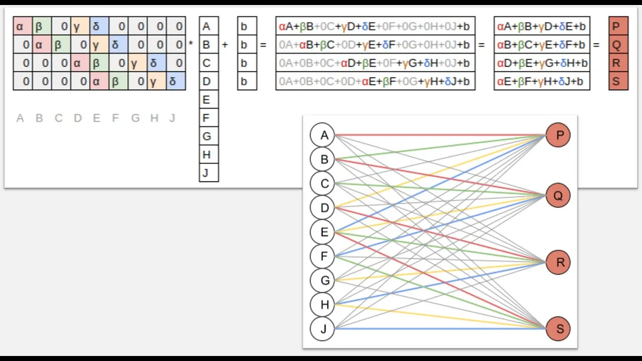
01:15:50.560 | So in other words P.

01:15:54.000 | Equals alpha times a beta times B gamma times D delta times a there it is.

01:16:04.640 | Plus B which is a bias OK so that's fine that's just a normal bias.

01:16:10.160 | So you can see how basically each of these output pixels is a result of some different linear equation.

01:16:18.640 | That makes sense and you can see these same four weights are being moved around because this is our convolutional kernel.

01:16:27.200 | Here's another way of looking at it from that.

01:16:30.440 | Which is here is a classic neural network view and so P now is result of multiplying every one of these inputs by a weight and then adding them all together except the gray ones.

01:16:47.640 | I got to have a value of zero right because remember P was only connected to A B D and E A B D and A.

01:17:01.720 | So in other words remembering that this represents a matrix multiplication.

01:17:09.400 | Therefore we can represent this as a matrix multiplication.

01:17:14.760 | So here is our list of pixels in our three by three image flattened out into a vector and here is a matrix vector multiplication plus bias.

01:17:27.960 | And then a whole bunch of them we're just going to set to zero.

01:17:32.640 | So you can see here we've got a zero zero zero zero zero which corresponds to zero zero zero zero zero.

01:17:42.000 | So in other words a convolution is just a matrix multiplication where two things happen.

01:17:49.600 | Some of the entries are set to zero all the time and all of the ones of the same color always have the same weight.

01:17:57.560 | So when you've got multiple things with the same weight that's called weight time.

01:18:03.720 | So clearly we could implement a convolution using matrix multiplication but we don't because it's slow.

01:18:12.120 | So in practice our libraries have specific convolution functions that we use and they're basically doing this.

01:18:22.600 | Which is this which is this equation which is the same as this matrix multiplication.

01:18:30.040 | And as we discussed we have to think about padding because if you have a three by three kernel and a three by three image then that can only create one pixel of output.

01:18:41.800 | There's only one place that this three by three can go.

01:18:45.320 | So if we want to create more than one pixel of output we have to do something called padding which is to put additional numbers all around the outside.

01:18:54.480 | So what most libraries do is that they just put a layer of zeros not a layer a bunch of zeros are all around the outside.

01:19:02.480 | So for a three by three kernel a single zero on every edge piece here.

01:19:08.360 | And so once you've padded it like that you can now move your three by three kernel all the way across and give you the same output size that you started with.

01:19:19.000 | Now as we mentioned in fast AI we don't normally necessarily use zero padding where possible.

01:19:25.720 | We use reflection padding although for these simple convolutions we often use zero padding because it doesn't matter too much in a big image.

01:19:34.680 | It doesn't make too much difference.

01:19:40.040 | OK so that's what a convolution is.

01:19:45.880 | So a convolutional neural network wouldn't be very interesting if it can only create top edges.

01:19:56.520 | So we have to take it a little bit further.

01:20:01.600 | So if we have an input.

01:20:09.960 | And it might be a standard kind of red green blue.

01:20:17.680 | Picture.

01:20:22.360 | Then we can create a kernel a three by three kernel.

01:20:31.960 | Like so.

01:20:33.840 | And then we could pass that kernel over all of the different pixels.

01:20:39.040 | But if you think about it we actually don't have a 2D input anymore.

01:20:43.040 | We have a 3D input a rank three tensor.

01:20:46.960 | So we probably don't want to use the same kernel values for each of red and green and blue because for example if we're creating a green frog detector we would want more activations on the green.

01:21:00.480 | Than we would on the blue or if we're trying to find something that can actually find a gradient that goes from green to blue then the different kernels for each channel need to have different values in.

01:21:12.640 | So therefore we need to create a.

01:21:16.400 | Three by three by three kernel.

01:21:22.960 | Okay, so this is still a kernel. And we're still going to vary it across the height and the width.

01:21:32.400 | But rather than doing an element wise modification of nine things we're going to do an element wise modification of twenty seven things three by three by three and we're still going to then add them up into a single number.

01:21:45.440 | So as we pass this cube over. This and the kind of like the little bit that's going to be sitting behind it.

01:21:55.200 | As we do that part of the convolution.

01:21:59.280 | It's still going to create just.

01:22:02.400 | One number as we do an element wise multiplication of all twenty seven and add them all together.

01:22:09.360 | So we can do that across the whole padded single unit padded input and so we started with one two three four five by five so we're going to end up with an output that's also.

01:22:23.440 | Five by five.

01:22:27.600 | But now our input was three channels and our output is only one channel.

01:22:33.920 | Now we're not going to be able to do very much with just one channel because all we've done now is found.

01:22:39.200 | The top edge how we're going to find a side edge and a gradient and an area of constant white.

01:22:48.160 | Well, we're going to have to create another kernel.

01:22:54.160 | And we're going to have to do that convolved over the input and that's going to create.

01:23:01.520 | Another five by five.

01:23:04.400 | And then we can just stack those together.

01:23:10.320 | Across this as another access and we can do that lots and lots of times.

01:23:15.200 | And that's going to give us.

01:23:19.760 | Another rank three tensor output.

01:23:24.240 | So that's what happens in practice that in practice we start with an input which is H.

01:23:32.240 | Which is H by W by images three.

01:23:39.760 | We pass it through a bunch of convolutional kernels that we can get to pick how many we want and it gives us back an output of.

01:23:50.240 | And it gives us back an output of height by width by however many kernels we had and so often that might be something like 16.

01:24:00.800 | In the first layer.

01:24:02.800 | And so now we've got 16 channels they called.

01:24:07.840 | 16 channels.

01:24:10.320 | Representing things like how much left and edge was on this pixel how much top edge was in this pixel how much blue to red gradient was on this level this set of 27.

01:24:22.560 | Nine pixels each with RGB and so then you can just do the same thing right you can have another.

01:24:29.280 | Bunch of.

01:24:31.600 | Colonels.

01:24:36.240 | And that's going to create another output.

01:24:38.400 | Frank three tensor again height by width by whatever might still be 16.

01:24:47.200 | Now what we really like to do is as we get deeper in the network we actually want to have more and more channels we want to be able to find like a richer and richer set of features so that after a few as we saw in this either in focus paper by layer four or five we've kind of got.

01:25:02.640 | Eyeball detectors and fur detectors and things right so you really need a lot of channels.

01:25:07.920 | So in order to avoid our memory going out of control.

01:25:11.920 | From time to time we create a convolution where we don't step over every single set of three by three.

01:25:21.840 | But instead we skip over two at a time.

01:25:26.400 | So we would start with a three by three centered at two comma two and then we jump over to two comma four two comma six two comma eight and so forth and that's called a stride.

01:25:39.280 | Two convolution.

01:25:42.160 | And so what that does is it looks exactly the same right it's still just a bunch of kernels.

01:25:53.760 | But we're just jumping over two at a time right we're skipping every alternate input pixel and so the output from that.

01:26:04.240 | Will be H over two by W over two and so when we do that we generally create twice as many kernels so we can now have say.

01:26:15.440 | Thirty two activations in each of those spots and so that's what modern convolutional neural networks kind of tend to look like right and so we can actually see that.

01:26:31.760 | If we go into our pets and we grab our CNN. Right and we're going to take a look at this particular cat so if we go X comma Y equals valid data set some index so it's just grab the zeroth or go to show and would print out the value of Y.

01:26:49.680 | Apparently this cat is of category main current so until a week ago I was not at all familiar that there's a cat called a main current having spent all week with this particular cat.

01:27:00.880 | I am now deeply familiar with this main current.

01:27:06.480 | So we can if we go learn dot summary. Remember that our input we asked for was three fifty two by three fifty two pixels.

01:27:17.920 | Generally speaking the very first convolution tends to have a stride too so after the first layer it's one seventy six by one seventy six.

01:27:26.680 | So this is learned summary will print out for you the output shape after every layer one seventy six by one seventy six and the first set of convolutions is has sixty four activations and we can actually see that if we type in learn.

01:27:44.600 | Got model. You can see here it's a two day con with three input channels and sixty four output channels.

01:27:54.840 | And a stride.

01:27:57.000 | Of two.

01:28:00.080 | And interestingly it actually starts with a kernel size of seven by seven so like nearly all of the convolutions are three by three see they're all three by three right for reasons we're talking about in part two we often use a larger kernel for the very first one.

01:28:14.320 | If you use a larger kernel you have to use more padding so we have to use kernel size in divided by two padding to make sure we don't lose anything anyway so.

01:28:26.440 | We now have sixty four output channels and since it was straight to it's now one seventy six by one seventy six and then.

01:28:34.560 | As we go along you'll see that from time to time.

01:28:38.720 | We have go from eighty eight by eighty eight to forty by forty four by forty four the grid size so that was a two day con and then when we do that we generally double the number of channels.

01:28:55.320 | So we keep going through a few more coms and they've as you can see they've got batch norm and really that's kind of pretty standard.

01:29:03.800 | And eventually we do it again now the strategy cons which again doubles we've now got five twelve by eleven by eleven.

01:29:13.400 | And.

01:29:15.440 | That's basically where we finish the main part of the network we end up with five twelve channels eleven by eleven.

01:29:24.560 | OK so we're actually at a point where we're going to be able to do this heat map now so let's try and work through it.

01:29:31.840 | Before we do I want to show you how you can do your own manual convolutions because it's kind of fun.

01:29:40.440 | So we're going to start with this picture of a main Coon.

01:29:44.400 | And I've created a convolutional kernel.

01:29:48.280 | And so as you can see this one has a right edge and a bottom edge with positive numbers and just inside that it's got negative numbers.

01:29:56.640 | So I'm thinking this should show me bottom right edges.

01:30:03.600 | So that's my tensor now one complexity is that that three by three kernel cannot be used for this purpose because I need two more dimensions.

01:30:17.920 | The first is I need the third dimension to say how to combine the red green and blue.

01:30:26.000 | So what I do is I say don't expand.

01:30:31.240 | This is my three by three and I pop another three on the start what don't expand does is it says create a three by three by three tensor by simply copying this one.

01:30:43.880 | Three times when honestly it doesn't actually copy it it pretends to have copied it you know but it just basically refers to the same block of memory so it kind of copies it in a memory efficient way.

01:30:55.760 | So this one here is now three copies of that and the reason for that is that I want to treat red and green and blue the same way for this little manual kernel I'm showing you.

01:31:10.040 | And then we need one more access because rather than actually having a separate kernel like I kind of printed these as if they were multiple kernels what we actually do is we use a rank for tensor.

01:31:23.680 | And so the very first access is for the every separate.

01:31:28.920 | Kernel that we have so this case I'm just going to create one kernel so to do a convolution I still have to put this unit access on the front.

01:31:38.520 | So you can see k dot shape is now one comma three comma three comma three so it's a three by three kernel there are three of them and then that's just the one kernel that I have so it kind of takes a while to get the feel for these.

01:31:53.040 | Higher dimensional tensors because we're not used to writing out the four D tensor but like just think of them like this a four D tensor is just a bunch of three D tensor sitting on top of each other okay.

01:32:06.240 | So this is our four D tensor and then you can just call.

01:32:12.720 | Conf 2D passing in some image and so the image I'm going to use is the first part of my validation data set and the kernel.

01:32:21.960 | There's one more trick which is that in PyTorch pretty much everything is expecting to work on a mini batch.

01:32:29.920 | Not on an individual thing.

01:32:32.760 | So in our case we have to create a mini batch of size one so our original image is three channels by three fifty two by three fifty two by width that's member PyTorch is channel by height by width.

01:32:46.480 | I want to create a mini so I need to create a rank for tensor.

01:32:51.000 | Where the first access is one in other words it's a mini batch of size one because that's what PyTorch expects so there's something you can do in both PyTorch and NumPy which is you can index into an array or a tensor with a special value none and that creates a new unit access.

01:33:11.200 | In that point point so T is my image of dimensions three by three fifty two by three fifty two T none is a rank for tensor a mini batch of one image of one by three by three fifty two by three fifty two and so now I can go con 2D.

01:33:29.280 | And get back.

01:33:33.920 | Specifically my main Coon.

01:33:39.440 | OK so that's how you can play around with convolutions yourself.

01:33:47.120 | So how are we going to do this to create a heat map.

01:33:50.840 | This is where things get fun.

01:34:00.960 | Remember what I mentioned was that I basically have like.

01:34:08.160 | My input.

01:34:11.120 | Red green blue and it goes through a bunch of convolutional layers I just write a little line to say a convolutional layer.

01:34:20.920 | To create activations which have more and more channels and eventually less and less smaller and smaller height by width.

01:34:35.720 | Until eventually remember we looked at the summary we ended up with something which was.

01:34:42.280 | Eleven by eleven by.

01:34:47.920 | Five twelve.

01:34:50.560 | And there's a whole there's a whole bunch more layers that we skipped over.

01:34:55.880 | Now there are.

01:35:04.080 | Thirty seven classes because remember data dot C is the number of classes we have and we can see that at the end here.

01:35:12.200 | We end up with thirty seven features in our model.

01:35:15.640 | So that means that we end up with a probability for every one of the thirty seven breeds of cat and dog.

01:35:23.160 | So it's a vector.

01:35:24.920 | Of length thirty seven that's our final output that we need because that's what we're going to compare.

01:35:29.760 | Implicitly to our one hot encoded matrix which will have a one in the location for main Coon.

01:35:38.760 | So somehow we need to get from this eleven by eleven by five twelve.

01:35:44.720 | To this thirty seven and so the way we do it is we actually take the average of every one of these eleven by eleven faces we just take the main.

01:35:57.720 | So we're going to take the main of this.

01:36:00.680 | First face take the main.

01:36:05.520 | That gets us one value and then we'll take the second of the five twelve faces and take that mean and that'll give us one more value.

01:36:13.400 | And so we'll do that for every face.

01:36:16.160 | And that will give us a.

01:36:19.280 | Five twelve long.

01:36:21.360 | Vector.

01:36:23.880 | And so now all we need to do is pop that through a single matrix multiply.

01:36:31.160 | Of five twelve.

01:36:33.320 | By thirty seven.

01:36:37.720 | And that's going to give us an output vector of length thirty seven.

01:36:42.040 | OK so this step here where we take the average of each face is called average pooling.

01:36:52.640 | So let's go back to our model and take a look here it is.

01:36:56.600 | Here is our final five twelve and here is we will talk about what a concave pooling is in part two for now we'll just focus on this.

01:37:05.360 | This is a fast speciality everybody else just does this average pool.

01:37:09.880 | Average pool duty with an output size of one.

01:37:13.040 | So here it is output average pool 2D with an output size of one.

01:37:20.320 | And then.

01:37:23.720 | Again there's a bit of a.

01:37:27.760 | Special faster I think that we actually have two layers here but normally people then just have the one.

01:37:33.120 | Linear layer.

01:37:34.800 | With the input of five twelve and the output of thirty seven.

01:37:41.840 | OK so what that means is that this little box over here.

01:37:47.480 | Where we want a one for Maine Coon we've got to have a box over here which needs to have a high value.

01:37:54.880 | In that place so that the lots will be low so if we're going to have a high value there.

01:38:01.560 | The only way to get it is with this matrix multiplication is that it's going to represent a simple weighted linear combination of all of the five hundred and twelve values here.

01:38:14.800 | So if we're going to be able to say I'm pretty confident this is a Maine Coon just by taking the weighted sum of a bunch of inputs those inputs are going to have to represent features like.

01:38:26.200 | How fluffy is it what color is its nose how long is its legs how point here it is all the kinds of things that can be used because for the other thing which figures out is this a bulldog it's going to use exactly the same.

01:38:41.520 | Kind of five twelve inputs with a different set of weights because that's all the matrix multiplication is right it's just a bunch of weighted sums a different weighted sum for each output.

01:38:54.760 | So therefore we know that this you know.

01:39:00.160 | Potentially dozens or even hundreds of layers of convolutions must have eventually come up with an eleven by eleven face.

01:39:09.920 | For each of these features saying and this little bit here.

01:39:15.920 | How much is that part of the image like a point here how much is it fluffy how much is it like a long leg how much is it like a very red nose right so that's what all of those things must represent so each face is what we call each of these.

01:39:34.640 | Represents a different feature.

01:39:39.840 | So the outputs of these we can think of as different features.

01:39:46.840 | So what we really want to know then is not so much what's the average across the eleven by eleven to get this set of outputs but what we really want to know is what's in each of these eleven by eleven spots.

01:40:03.360 | So what if instead of averaging across the eleven by eleven let's instead average across.

01:40:11.040 | The five hundred and twelve if we average across the five hundred and twelve that's going to give us a single eleven by eleven matrix.

01:40:20.600 | And each item each grid point in that eleven by eleven matrix will be the average of how activated was that area when it came to figuring out that this was a main kun.

01:40:34.360 | How many signs of main kunishness was there in that part of the eleven by eleven grid.

01:40:43.720 | And so that's actually what we do to create our heat map so I think maybe the easiest way is to kind of work backwards.

01:40:51.880 | Here's our heat map.

01:40:54.000 | And it comes from something called average activations and it's just a little bit of matplotlib and fastai fastai to show the image and then matplotlib to take the heat map which we passed in which was called average activations H.M. for heat map.

01:41:12.840 | Alpha point six means make it a bit transparent.

01:41:16.640 | In that plot live extent means expand it from eleven by eleven to three fifty two by three fifty two.

01:41:24.200 | He is by linear interpolation so it's not all blocky and use a different color map to kind of highlight things such as the matplotlib is not important.

01:41:31.760 | The key thing here is that average activations is the eleven by eleven matrix we wanted.

01:41:37.360 | Here it is average activations touch shape is eleven by eleven.

01:41:42.520 | So to get there we took the mean of activations across dimension zero which is what I just said in PyTorch the channel dimension is the first dimension so the main across dimension zero took us from something of size five twelve by eleven by eleven as promised to something of eleven by eleven.

01:42:02.400 | So therefore activations acts contains the activations were averaging where did they come from.

01:42:10.120 | They came from something called a hook.

01:42:13.240 | So a hook is a really cool more advanced PyTorch feature that lets you as the name suggests hook into the PyTorch machinery itself and run any arbitrary Python code you want to.

01:42:32.680 | It's a really amazing and nifty thing because you know normally when we do a forward pass through a PyTorch module it gives us this set of outputs but we know that in the process it's calculated these.

01:42:50.560 | So why would I what I would like to do is I would like to hook into that forward pass and tell PyTorch hey when you calculate this can you store it for me please.

01:43:02.720 | So what is this this is the output of the convolutional part of the model so the convolutional part of the model which is everything before the average pool.

01:43:12.840 | Is basically all of. That. And so thinking back to transfer learning.

01:43:23.720 | I remember with transfer learning.

01:43:27.000 | We actually.

01:43:30.480 | Cut off everything after the convolutional part of the model and replaced it with our own little bit.

01:43:36.960 | So with fast AI the original convolutional part of the model is always going to be the first thing in the model and specifically it's always going to be called.

01:43:50.480 | Assuming so in this case I'm taking my model and I'm just going to call it M right so you can see.

01:43:59.680 | M is this. Big thing. But always. At least in faster AI always M zero.

01:44:09.880 | Will be the convolutional part of the model so in this case we created a.

01:44:15.400 | Let's go back and see we created a resident 34.

01:44:19.160 | So the main part of the resident 34 the pre trained bit we hold onto is in M zero and so this is basically it this is a print out of the resident 34 and at the end of it there is the 512 activations.

01:44:33.520 | So what in other words what we want to do is we want to grab.

01:44:39.160 | M zero and we want to hook its output so this is a really useful thing to be able to do so fast AI is actually created something to do it.

01:44:48.840 | For you which is literally you say hook output and you pass in the pipe watch module that you want to hook the output of and so most of the most likely the thing you want to hook is.

01:45:00.720 | The convolutional part of the model and that's always going to be M zero or learned up model zero.

01:45:07.800 | So we give that hook a name.

01:45:10.320 | Don't worry about this part will learn about it next week.

01:45:13.320 | So having hooked the output we now need to actually do the forward pass right and so remember in PI torch to actually get it to calculate something which is called doing the forward pass you just act as if the model is a function.

01:45:27.400 | So we just pass in our X X mini batch so we already had.

01:45:34.280 | A main Coon image called X right but we can't quite pass that into our model it has to be normalized and turned into a mini batch and put onto the GPU.

01:45:48.280 | So fast AI has a thing called a data bunch which we haven't data and you can always say data dot one item to create a mini batch with one thing in it and as an exercise at home you could try to.

01:46:02.240 | Create a mini batch without using data dot one item to make sure that you kind of learn how to normalize and stuff yourself if you want to, but this is how you can create a.

01:46:12.600 | Mini batch with just one thing in it and then I can pop that onto the GPU by saying dot CUDA.

01:46:19.720 | That's what I passed in my model and so the predictions I get out.

01:46:23.800 | Actually don't care about that 'cause the predictions is.

01:46:30.400 | The predictions is this thing which is not what I want right so I'm not actually going to do anything with the predictions. The thing I care about is the hook that I just created.

01:46:40.920 | Now one thing to be aware of is that when you hook something in pytorch that means every single time you run that model.

01:46:50.040 | Assuming your hooking outputs, it's storing those outputs and so you want to remove the hook when you've got what you want 'cause otherwise if you use the model again, it's going to keep looking more and more outputs, which will be slow and memory intensive.

01:47:02.360 | So we've created this thing. Python calls it a context manager. You can use any hook as a context manager at the end of that with block. It'll remove the hook.

01:47:15.600 | So we got our hook. And so now pytorch hooks sorry fast AI hooks always give you something called or at least the output hooks always give you something called dot stored, which is where it stores away. The thing you asked it to hook and so that's where the activations.

01:47:32.480 | Now OK, so we did a forward pass after hooking the output of the convolutional section of the model. We grabbed what it stored.

01:47:42.360 | We check the shape. It was 512 by 11 by 11 as we predicted.

01:47:48.040 | We then took the main of the channel access to get an 11 by 11 tensor.

01:47:56.760 | And then. If we look at that.

01:48:00.240 | That's our picture, so there's a lot to unpack.

01:48:04.040 | Right, a lot to unpack, but if you take your time going through these two sections, the convolution kernel section and the heat map section of this notebook like running those lines of code and changing them around a little bit.

01:48:17.960 | And remember, the most important thing to look at is shape. You might have noticed when I'm showing you these notebooks are very often print out the shape and we look at the shape. You want to be looking at how many axes are there.

01:48:30.600 | That's the rank of the tensor and how many things are there in each axis and try and think why I tried going back to the print out of the summary.

01:48:41.160 | Try going back to the actual list of the layers and try and go back and think about the actual picture we drew and think about what's actually going on.

01:48:50.800 | OK. So that's a lot of technical content, so what I'm going to do now is switch from technical content to something much more important unless we have some questions first.

01:49:05.600 | OK, because in the next lesson, we're going to be looking at generative models, both text and image generative models.

01:49:20.920 | And generative models are where you can create a new piece of text or a new image or a new video or a new sound.

01:49:34.280 | And as you probably are aware, this is the area that deep learning has developed the most in in the last 12 months.

01:49:42.040 | So we're now at a point where we can generate realistic looking videos, images, audio, and to some extent, even text.

01:49:57.120 | And so there are many things in in this journey which have ethical considerations, but perhaps this area of generative modeling is one of the largest ones.

01:50:09.640 | So before I got into it, I wanted to specifically touch on ethics and data science.

01:50:17.360 | Most of the stuff I'm showing you actually comes from Rachel and Rachel has a really cool TEDx San Francisco talk that you can check out on YouTube and a more extensive analysis of ethical principles and bias principles in AI, which you can find at this talk here.

01:50:38.400 | And she has a playlist that you can check out.

01:50:42.280 | We've already touched on an example of bias, which was this gender shades study, where if you remember, for example, lighter male skin people on IBM's main computer vision system, 99.7 percent accurate and darker females are some hundreds of times less accurate in terms of error.

01:51:08.600 | So like extraordinary differences. And so it's interesting to kind of like, OK, it's first of all important to be aware that not only can this happen technically, that this can happen on a massive companies rolled out publicly available, highly marketed system that hundreds of quality control people have studied and lots of people are using.

01:51:31.760 | It's out there in the world. They all look kind of crazy.

01:51:40.160 | And so it's interesting to think about why. And so one of the reasons why is that the data we feed these things, we tend to use me included a lot of these data sets kind of unthinkingly.

01:51:52.800 | But like ImageNet, which is the basis of like a lot of the computer vision stuff we do, is over half American and Great Britain.

01:52:03.040 | Like when it comes to the countries that actually have most of the population in the world.

01:52:11.160 | I can't even see them here. They're somewhere in these impossibly thin lines. Because remember, these data sets are being created almost exclusively by people in US, Great Britain and nowadays increasingly also China.

01:52:28.040 | So there's a lot of bias in the content we're creating because of a bias in the kind of people that are creating that content, even when in theory it's being created in a very kind of neutral way.

01:52:40.040 | But you can't argue with the data, right? It's obviously not neutral at all.

01:52:47.200 | And so when you have biased data creating biased algorithms, you then need to say, like, what are we doing with that?

01:52:55.920 | So we've spent a lot of time talking about image recognition.

01:52:59.520 | So a couple of years ago, this company, DeepClint, advertised their image recognition system, which can be used to do mass surveillance on large crowds of people.

01:53:11.960 | Find any person passing through who is a person of interest in theory.

01:53:18.480 | And so putting aside even the question of like, is it a good idea to have such a system?

01:53:26.000 | You've got to think, is it a good idea to have such a system where certain kinds of people are 300 times more likely to be misidentified?

01:53:35.120 | And then thinking about it. So this is now starting to happen in America. These systems are being rolled out.

01:53:42.600 | And so there are now systems in America that will identify a person of interest in a video and send a ping to the local police.

01:53:53.760 | And so these systems are extremely inaccurate and extremely biased.

01:53:59.280 | And what happens then, of course, is if you're in a predominantly black neighborhood where the probability of successfully recognizing you is much lower

01:54:10.560 | and you're much more likely to be surrounded by black people.

01:54:13.960 | And so suddenly all of these black people are popping up as persons of interest or in a video of a person of interest.

01:54:21.760 | All the people in the video are all recognized as in the vicinity as a person of interest.

01:54:26.920 | You suddenly get all these pings going off the local police department, causing the police to run down there and therefore likely to lead to a larger number of arrests,

01:54:37.320 | which is then likely to feed back into the data being used to develop the systems.

01:54:42.520 | So this is happening right now. And so, like, thankfully, a very small number of people are actually bothering to look into these things.

01:54:50.440 | I mean, ridiculously small, but at least it's better than nothing.

01:54:53.240 | And so, for example, one of the best ways that people get publicity is to do kind of funny experiments like let's try the mugshot image recognition system that's being widely used

01:55:07.480 | and try it against the members of Congress and find out that there are 28 members of Congress who would have been identified by this system.

01:55:15.880 | Obviously incorrectly. Oh, I didn't know that.

01:55:21.280 | OK, members of black members of Congress. Not at all surprised to hear that. Thank you, Rachel.

01:55:28.360 | We see this kind of bias in a lot of the systems we use, not just image recognition, but text translation.

01:55:35.120 | When you convert she is a doctor, he is a nurse into Turkish, you quite correctly get a gender in specific pronoun because that's what Turkish uses.

01:55:45.080 | You could then take that and feed it back into Turkish with your gender in specific pronoun and you will now get he is a doctor.

01:55:52.040 | She is in this. So the bias again, this is in a massively widely rolled out, carefully studied system.

01:56:00.440 | And it's not like even these kind of things like a little one off things that then get fixed quickly.

01:56:05.640 | These issues have been identified in Google Translate for a very long time and they're still there and they don't get fixed.

01:56:14.200 | So the. The kind of results of this are, in my opinion, quite terrifying because what's happening is that in many countries,

01:56:26.200 | including America, where I'm speaking from now, algorithms are increasingly being used for all kinds of public policy, judicial and so forth purposes.

01:56:37.480 | For example, there's a system called Compass, which is very widely used to decide who's going to jail.

01:56:43.640 | And it does that in a couple of ways. It tells judges what sentencing guidelines they should use for particular cases.

01:56:50.640 | And it tells them also which people the system says should be let out on bail.

01:56:58.760 | But here's the thing, white people, it keeps on saying, let this person out, even though they end up reoffending and vice versa.

01:57:07.720 | It's systematically like out by double compared to what it should be in terms of getting it wrong with white people versus black people.

01:57:19.040 | So this is like kind of horrifying because I mean, amongst other things, the data that it's using in this system is literally asking people questions about things like,

01:57:34.600 | did any of your parents ever go to jail? Do any of your friends do drugs?

01:57:39.880 | Like they're asking questions about other people who they have no control over. So not only are these systems biased, very systematically biased,

01:57:51.640 | but they're also being done on the basis of data, which is totally out of your control.

01:57:57.640 | So this is kind of did you want to add something to that?

01:58:01.520 | Oh, yeah, are your parents divorced is another question that's being used to decide whether you go to jail or not.

01:58:07.480 | So when we raise these issues kind of on Twitter or in talks or whatever, there's always a few people, always white men,

01:58:18.600 | a few people who will always say, like, that's just the way the world is, that's just reflecting what the data shows.

01:58:26.480 | But when you actually look at it, it's not right. It's actually systematically erroneous and systematically erroneous against people of color minorities,

01:58:39.560 | the people who are less involved in creating the systems that these products are based on.

01:58:47.160 | Sometimes this can go a really long way. So, for example, in Myanmar, there was a genocide of the Rohingya people and that genocide was very heavily created by Facebook.

01:59:03.320 | Not because anybody at Facebook wanted it. I mean, heavens know. I know a lot of people at Facebook. I have a lot of friends at Facebook.

01:59:10.040 | They're really trying to do the right thing, right? They're really trying to create a product that people like.

01:59:15.240 | But not in a thoughtful enough way, because when you roll out something, we're literally in Myanmar, a country that most people didn't have most.

01:59:25.560 | Maybe half of people didn't have electricity until very recently. And you say, hey, you can all have free Internet as long as it's just Facebook.

01:59:34.920 | You've got to think carefully about what you're doing, right? And then you use algorithms to feed people the stuff they will click on.

01:59:42.000 | And of course, what people click on is stuff which is controversial, stuff that makes their blood boil.

01:59:48.320 | So when they actually started asking the generals in the Myanmar army that were literally throwing babies onto bonfires,

01:59:57.200 | they were saying, we know that these are not humans. We know that they are animals because we read the news, we read the Internet.

02:00:06.440 | And because this is the stories that the algorithms are pushing, and the algorithms are pushing the stories because the algorithms are good.

02:00:15.840 | They know how to create eyeballs, how to get people watching and how to get people clicking.

02:00:21.440 | And again, nobody at Facebook said, let's cause a massive genocide in Myanmar.

02:00:28.480 | They said, let's maximize the engagement of people in this new market on our platform, right?

02:00:36.840 | So they very successfully maximized engagement. Yes, please.

02:00:45.960 | It's just it's important to note people warned executives at Facebook how the platform was being used to incite violence as far back as 2013, 2014, 2015 and 2015.

02:00:57.520 | Someone even warned executives that Facebook could be used in Myanmar in the same way that the radio broadcast were used in Rwanda during the Rwandan genocide.

02:01:07.440 | And as of 2015, Facebook only had four contractors who spoke Burmese working for them.

02:01:15.480 | They really did not put many resources into the issue at all, even though they were getting very, very alarming warnings about it.

02:01:24.480 | So I mean, so why does this happen? A part of the issue is that ethics is complicated and you will not find Rachel or I telling you how to do ethics.

02:01:37.720 | You know, how do you fix this? We don't know. We can just give you kind of things to think about.

02:01:45.160 | Another part of the problem we keep hearing is it's not my problem. I'm just a researcher. I'm just a techie. I'm just holding a data set.

02:01:53.440 | I'm not part of the problem. I'm part of this foundation that's far enough away that I can imagine that I'm not part of this.

02:02:00.680 | But. You know, if you're creating image net and you wanted to be successful, you want lots of people to use it, you want lots of people to build products on it, lots of people to do research on top of it.

02:02:12.160 | If you're trying to create something that people are using, you want them to use, then please try to make it something that won't cause massive amounts of harm and doesn't have massive amounts of bias.

02:02:23.400 | And it can actually come back and bite you in the ass, right? The Volkswagen engineer who ended up actually encoding the thing that made them systematically cheat on their diesel emissions tests, on their pollution tests, ended up in jail.

02:02:40.880 | Not because it was their decision to cheat on the tests, but because their manager told them to write that code and they wrote the code and therefore they were at the ones that ended up being criminally responsible and they were the ones that were jailed.

02:02:56.080 | So if you do in some way a shitty thing that ends up causing trouble, that can absolutely come back around and get you in trouble as well.

02:03:07.600 | Sometimes it can cause huge amounts of trouble. So if we go back to World War II, then this was one of the first great opportunities for IBM to show off their amazing tabulating system.

02:03:22.560 | And they had a huge client in Nazi Germany. And Nazi Germany used this amazing new tabulating system to encode all of the different types of Jews that they had in the country and all the different types of problem people.

02:03:35.920 | So Jews were 8, Gypsies were 12, then different outcomes were coded, executions were a 4, death in a gash chamber was 6, a Swiss judge ruled that IBM was actively involved facilitating the commission of these crimes against humanity.

02:03:59.880 | So there are absolutely plenty of examples of people building data processing technology that are directly causing deaths, sometimes millions of deaths, right?

02:04:15.560 | So we don't want to be one of those people. And so you might have thought, oh, you know, I'm just creating some data processing software and somebody else is thinking I'm just a sales person and somebody else is thinking I'm just the biz dev person opening new markets, but it all comes together, right?

02:04:29.320 | So we need to care. And so one of the things we need to care about is getting humans back in the loop, right?

02:04:39.240 | And so when we pull humans out of the loop is one of the first times that trouble happens.

02:04:44.560 | I don't know if you remember. I remember this very clearly when I first heard that Facebook was firing the human editors that were responsible for basically curating the news that ended up on the Facebook pages.

02:05:01.080 | And I got to say at the time, I thought that's a recipe for disaster because I've seen again and again that humans can be the person in the loop that can realize this isn't right.

02:05:12.920 | You know, it's very hard to create an algorithm that can recognize this isn't right or else humans are very good at that.

02:05:19.960 | And we saw that's what happened. Right. After Facebook fired the human editors, the nature of stories on Facebook dramatically changed.

02:05:28.440 | But you started seeing this proliferation of conspiracy theories and the kind of the algorithms went crazy with recommending more and more controversial topics.

02:05:37.600 | And of course, that changed people's consumption behavior, causing them to want more and more controversial topics.

02:05:46.200 | So where one of the really interesting places this comes in and Kathy O'Neill, who's got a great book called weapons of math destruction.

02:05:55.840 | Thank you, Rachel. And many others have pointed out is that what happens to algorithms is that they end up impacting people.

02:06:07.560 | For example, compass sentencing guidelines go to a judge. Now, you can say the algorithm is very good.

02:06:16.000 | I mean, in compass, this case, it isn't. It actually turned out to be about as bad as random because it's a black box and all that.

02:06:23.720 | But even if it was very good, you could then say, well, you know, the judge is getting the algorithm.

02:06:28.680 | Otherwise, they'd just be getting a person. People also give bad advice. So what humans respond differently to algorithms.

02:06:36.320 | It's very common, particularly for a human that is not very familiar with the technology themselves, like a judge to say, like, oh, that's what the computer says.

02:06:46.520 | The computer looked it up and it figured this out. It's extremely difficult to get a non-technical audience to look at a computer recommendation and come up with a nuanced decision making process.

02:07:01.480 | So what we see is that algorithms are often put into place with no appeals process.

02:07:08.280 | They're often used to massively scale up decision making systems because they're cheap.

02:07:15.400 | And then the people that are using the outputs of those algorithms tend to give them more credence than they deserve because very often they're being used by people that don't have the technical competence to judge them themselves.

02:07:26.720 | So great example, right, was here's an example of somebody who lost their health care and they lost their health care because of an error in a new algorithm that was systematically failing to recognize that there are many people that need help with, was it Alzheimer's?

02:07:48.960 | Cerebral Palsy and Diabetes. Thanks, Rachel. And so this system, which had this this error that was later discovered, was cutting off these people from the home care that they needed so that cerebral palsy victims no longer had the care they needed.

02:08:04.680 | So their life was destroyed, basically. And so when the person that created that algorithm with the error was asked about this and was specifically said, should they have found a better way to communicate the system, the strength, the failures and so forth?

02:08:23.920 | He said, yeah, I should probably also dust under my bed. That was there. That was the level of interest they had. And this is extremely common. I hear this all the time. And it's much easier to kind of see it from afar and say, OK, after the problems happened, I can see that that's a really shitty thing to say.

02:08:42.560 | But it can be very difficult when you're kind of in the middle of it. I just want to say one more thing about that example, and that's that this was a case where it was separate.

02:08:53.760 | There was someone who created the algorithm. Then I think different people implemented the software. And this is in use in over half of the 50 states.

02:09:00.840 | And then there was also the particular policy decisions made by that state. And so this is one of those situations where nobody felt responsible because the algorithm creators like, oh, no, it's the policy decisions of the state that were bad.

02:09:13.720 | And the state can be like, oh, no, it's the ones who implemented the software. And so everyone just kind of pointing fingers and not taking responsibility.

02:09:23.080 | And, you know, in some ways, maybe it's unfair, but I would argue the person who is creating the data set and the person who is implementing the algorithm is the person best placed to get out there and say, hey, here are the things you need to be careful of and make sure that they're a part of the implementation process.

02:09:44.280 | So we've also seen this with YouTube, right? It's kind of similar to what happened with Facebook. And we're now seeing we've heard examples of students watching the fast AI courses who say, hey, Jeremy and Rachel, watching the fast AI courses really enjoyed them.

02:09:58.920 | And at the end of one of them, the YouTube autoplay fed me across to a conspiracy theory.

02:10:05.960 | And what happens is that once the system decides that you like the conspiracy theories, it's going to just feed you more and more.

02:10:13.040 | And then what happens is that please go on just briefly, you don't you don't even have to like conspiracy theories.

02:10:21.840 | The goal is to get as many people hooked on conspiracy theories as possible is what the algorithm is trying to do, kind of whether or not you've expressed interest.

02:10:30.280 | Right. And so the interesting thing, again, is I know plenty of people involved in YouTube recommendation systems, none of them are wanting to promote conspiracy theories.

02:10:38.440 | But people click on them, right? And people share them.

02:10:43.360 | And what tends to happen is also people that are into conspiracy theories consume a lot more YouTube media.

02:10:51.600 | So it actually is very good at finding a market that watches a lot of hours of YouTube and that it makes that market watch even more.

02:10:59.120 | So this is an example of a feedback loop and the New York Times is now describing YouTube as perhaps the most powerful radicalizing instrument of the 21st century.

02:11:10.640 | I can tell you my friends that worked on the YouTube recommendation system did not think they were creating the most powerful radicalizing instrument of the 21st century.

02:11:21.120 | And to be honest, most of them today, when I talk to them, still think they're not. They think it's all bullshit, you know, not all of them, but a lot of them now are at the point where they just feel like they're the victims here.

02:11:35.560 | People are unfairly, you know, they don't get it. They don't understand what we're trying to do.

02:11:39.920 | It's very, very difficult when you're right out there in the heart of it.

02:11:43.560 | So you've got to be thinking from right at the start, what are the possible unintended consequences of what you're working on?

02:11:50.640 | And as the technical people involved, how can you get out in front and make sure that people are aware of them?

02:11:57.840 | And I just also wanted to say that in particular, many of these conspiracy theories are promoting white supremacy.

02:12:03.240 | They're, you know, kind of far right ethno-nationalism, anti-science. And I think, I don't know, maybe five or ten years ago, I would have thought conspiracy theories are more a more fringe thing.

02:12:14.040 | But we're seeing the kind of huge societal impact it can have for many people to believe these.

02:12:19.520 | Yeah. And, you know, partly it's you see them on YouTube all the time. It starts to feel a lot more normal.

02:12:25.520 | So one of the things that people are doing to try to say, like, how to fix this problem is to explicitly get involved in talking to the people who might or will be impacted by the kind of decision making processes that you're enabling.

02:12:38.640 | So, for example, there was a really cool thing recently where literally statisticians and data scientists got together with people who had been inside the criminal system.

02:12:51.560 | I had gone through the bail and sentencing process of criminals themselves and talking to the lawyers who worked with them and put them together with the data scientists and actually kind of put together a timeline of how exactly does it work and where exactly the places that there are inputs and how do people respond to them and who's involved.

02:13:10.480 | This is really cool, right? This is the only way for you as a kind of a data product developer to actually know how your data products going to be working. A really great example of somebody who did a great job here was Evan Estola at Meetup who said, hey, a lot of men are going to our tech meetups.

02:13:32.120 | And if we use a recommendation system naively, it's going to recommend more tech meetups to men, which is going to cause more men to go to them.

02:13:40.640 | And then when women do try to go, they'll be like, oh, my God, there's so many men here, which is going to cause more men to go to the tech meetups.

02:13:48.320 | Yeah, yeah. So showing recommendations to men and therefore not showing them to women. Yes, yeah.

02:13:55.200 | So so what Evan and meetup decided was to make an explicit product decision that this would not even be representing the actual true preferences of people.

02:14:08.480 | It would be creating a runaway feedback loop. So let's explicitly stop it right before it happens and and not recommend less meetups to women and tech meetups, women and more tech meetups to men.

02:14:23.000 | And so I think that's that's just it's really cool. It's like it's saying we don't have to be slaves to the algorithm.

02:14:28.320 | We actually get to decide. Another thing that people can do to help is regulation.

02:14:36.760 | And normally when we kind of talk about regulation, there's a natural reaction of like, how do you regulate these things?

02:14:42.400 | That's ridiculous. You can't regulate A.I. But actually, when you look at it again and again and this fantastic paper called Datasheets for Data Sets,

02:14:51.400 | has lots of examples of this. There are many, many examples of industries where people thought they couldn't be regulated.

02:14:58.200 | People thought that's just how it was like cars. People died in cars all the time because they literally had sharp metal knobs on dashboards.

02:15:06.520 | Steering columns weren't collapsible. And all of the discussion in the community was that's just how cars are.

02:15:13.960 | And when people die in cars, it's because of the people. But then eventually the regulations did come in.

02:15:19.600 | And today driving is dramatically safer like dozens and dozens of times safer than it was before.

02:15:27.800 | So often there are things we can do through policy. So to summarize.

02:15:34.840 | We are part of the point three to point five percent of the world that knows how to code.

02:15:41.400 | We have a skill that very few other people do. Not only that, we now know how to code deep learning algorithms,

02:15:47.000 | which is like the most powerful kind of code I know. So I'm hoping that we can explicitly think about like at least not making the world worse

02:15:56.320 | and perhaps explicitly making it better. And so why is this interesting to you as an audience in particular?

02:16:03.960 | And that's because fast AI in particular is trying to make it easy for domain experts to use deep learning.

02:16:12.520 | And so this picture of the goats here is an example of one of our international fellows from a previous course who was a goat dairy farmer

02:16:21.480 | and told us that they were going to use deep learning on their remote Canadian island to help study other disease in goats.

02:16:30.240 | And to me this is a great example of like a domain experts problem which nobody else even knows about,

02:16:36.240 | let alone know that it's a computer vision problem that can be solved with deep learning.

02:16:40.080 | So in your field, whatever it is, you probably know a lot more now about the opportunities in your field to make it a hell of a lot better than it was before.

02:16:52.960 | You'll probably be able to come up with all kinds of cool product ideas, right, maybe build a startup or create a new product group in your company or whatever.

02:17:01.800 | But also, please be thinking about what that's going to mean in practice and think about where can you put humans in the loop, right?

02:17:10.600 | Where can you put those pressure release valves? Who are the people you can talk to who could be impacted, who could help you understand, right?

02:17:18.760 | And get the kind of humanities folks involved to understand history and psychology and sociology and so forth.

02:17:25.560 | So that's our plea to you. If you've got this far, you're definitely at a point now where you're ready to, you know, make a serious impact on the world.

02:17:34.600 | So I hope we can make sure that that's a positive impact. See you next week.

02:17:38.360 | (audience applauds)

02:17:41.360 | (audience applauds)

Lesson 6: Deep Learning 2019 - Regularization; Convolutions; Data ethics

Chapters