Lesson 3: Practical Deep Learning for Coders 2022

00:00:00.000 | Hi everybody and welcome to lesson three of practical deep learning for coders

00:00:04.580 | we did a quick survey this week to see how people feel that the course is tracking and

00:00:11.900 | Over half a few think it's about right-paced and of the rest who aren't

00:00:18.320 | Some of you think it's a bit slow and some of you think it's a bit to sorry

00:00:21.960 | I'm gonna think it's a bit slow and some of you think it's a bit fast

00:00:23.920 | So hopefully we're that's about the best we can do

00:00:27.520 | Generally speaking the first two lessons are a little more easy pacing for anybody who's already familiar with the kind of

00:00:34.220 | basic technology pieces and then the later lessons get you know more into kind of some of the foundations and today

00:00:41.820 | we're going to be talking about

00:00:43.820 | You know things like the matrix multiplications and gradients and capitalists and stuff like that

00:00:50.400 | So for those of you who are more mathy and less computer II you might find this one more comfortable and vice-a-versa

00:00:57.240 | so

00:00:59.240 | Remember that there is a

00:01:04.360 | official course updates thread where you can see all the up-to-date info about

00:01:09.820 | Everything you need to know and of course the course website

00:01:13.400 | As well so by the time you know you watch the video of the lesson

00:01:19.600 | It's pretty likely that if you come across a question or an issue somebody else will have so definitely search

00:01:25.480 | the forum and check the facts

00:01:27.480 | First and then of course feel free to ask a question yourself on the forum if you can't find your answer

00:01:32.960 | One thing I did want to point out which you'll see in the lessons thread and the course website is

00:01:39.760 | There is also a lesson zero

00:01:42.840 | lesson zero is

00:01:45.480 | based heavily on

00:01:48.960 | Radix book meta learning which internally is based heavily on all the things that I've said over the years about how to learn fast AI

00:01:56.000 | It's we try to make the course full of

00:01:59.080 | Tickbits about the science of learning itself and put them into the course

00:02:04.400 | It's a different course to probably any other you've taken and it's I strongly recommend

00:02:10.600 | Watching lesson zero as well. The last bit of lesson zero is about how to set up a Linux box from scratch

00:02:18.040 | which you can happily skip over unless that's of interest, but the rest of it is

00:02:21.260 | Full of juicy information that I think you'll find useful

00:02:25.480 | So the basic idea of

00:02:29.120 | What to do to do a faster AI lesson is?

00:02:33.480 | Watch the lecture

00:02:36.680 | And I generally you know on the video recommend watching it all the way through

00:02:40.920 | without stopping once and then go back and

00:02:45.000 | Watch it with lots of pauses running the notebook as you go because otherwise you're kind of like running the notebook

00:02:50.800 | Without really knowing where it's heading if that makes sense

00:02:55.160 | And the idea of running the notebook is is you you know, there's a few notebooks you could go through

00:03:00.840 | So obviously there's the book so going through chapter one of the book going through chapter two of the book as notebooks

00:03:06.640 | running every code cell and

00:03:09.320 | Experimenting with inputs and outputs to try and understand what's going on

00:03:14.760 | And then trying to reproduce those results

00:03:17.780 | And then trying to repeat the whole thing with a different data set and if you can do that last step, you know, that's

00:03:25.120 | Quite a stretch goal particularly at the start of the course because there's so many new concepts

00:03:30.200 | But that really shows that you you've got it sorted now first third bit reproduce results

00:03:35.300 | I recommend using you'll find in the fastbook repo. So the repository for the book. There is a special folder called

00:03:44.120 | Clean and clean contains all of the same chapters of the book

00:03:47.760 | But with all of the text removed except for headings and all the outputs removed

00:03:53.160 | And this is a great way for you to test your understanding of the chapter is before you run each cell

00:04:00.440 | Charter say to yourself. Okay, what's this for?

00:04:03.440 | And what's it going to output if anything and if you kind of work through that slowly

00:04:09.560 | That's a great way at any time. You're not sure you can jump back to the

00:04:13.240 | Version of the notebook with a text to remind yourself and then head back over to the clean version

00:04:18.580 | So there's an idea for something which a lot of people find really useful for self-study I

00:04:27.640 | Say self-study, but of course as we've mentioned before

00:04:31.280 | The best kind of study is

00:04:34.640 | Study done to some extent with others for most people

00:04:37.800 | You know the research shows that you're more likely to stick with things if you're doing it

00:04:43.400 | That's kind of a bit of a social activity there. The forums are a great place to find and create

00:04:49.240 | Study groups and you'll also find on the forums a link to our discord server

00:04:56.080 | So yes our discord server where there are some study groups there as well

00:05:01.360 | so I'd you know in person study groups virtual study groups are a great way to

00:05:06.000 | You know really make good progress and find other people at a similar level to you

00:05:11.720 | if there's not a

00:05:14.560 | Study group going at your level in your area in your time zone

00:05:18.320 | Create one. So just post something saying hey, let's create a study group

00:05:22.280 | So this week there's been a lot of fantastic activity. I can't show all of it. So what I did was I used the

00:05:31.520 | summary functionality in the forums to grab all of the things with the highest votes and so I was quickly show a few of those we

00:05:37.160 | have a

00:05:38.200 | Marvel detector created this week

00:05:40.640 | Identify your favorite Marvel character. I

00:05:44.480 | Love this a rock-paper-scissors game where you actually use pictures of the rock-paper-scissors symbols and apparently

00:05:52.280 | The computer always loses. That's my favorite kind of game

00:05:57.080 | There is a lot of Elon around so very handy to have an Elon detector to you know

00:06:02.000 | Either find more of him if that's what you need or maybe less of him

00:06:05.440 | I thought this one is very interesting. I love these kind of really interesting ideas. It's like gee

00:06:12.580 | I wonder if this would work. Can you predict the average?

00:06:15.880 | temperature of an area based on a

00:06:20.480 | aerial photograph

00:06:22.720 | And the eye and apparently the answer is yeah, actually you can predict it pretty well here in Brisbane

00:06:28.320 | It was predicted. I believed it was in one and a half

00:06:30.680 | Celsius

00:06:33.360 | I think this student is actually a genuine meteorologist if I remember correctly he built a cloud detector

00:06:39.840 | So then building on top of the what's your favorite Marvel character? There's now also an is it a Marvel character

00:06:48.160 | My daughter loves this one. What dinosaur is this and I'm not as good about dinosaurs as I should be I feel like there's

00:06:54.920 | Ten times more dinosaurs than there was when I was a kid, so I'd never know their names. This is very handy

00:07:01.360 | This is cool. Choose your own adventure where you choose your path using facial expressions

00:07:06.800 | And I think this music genre classification

00:07:10.840 | Is also really cool

00:07:15.520 | Brian Smith created a Microsoft power app

00:07:19.200 | Application that actually runs on a mobile phone. That's pretty cool

00:07:23.400 | I wouldn't be surprised to hear that Brian actually works at Microsoft so also an opportunity to promote

00:07:28.880 | his own stuff there

00:07:31.400 | I thought this art movement classifier was interesting in that like there's a really interesting discussion on the forum about

00:07:37.040 | What it actually shows about similarities between different art movements

00:07:42.400 | And I thought this reduction detector project was really was really cool

00:07:47.280 | As well, and there's a whole tweet thread and blog post and everything about this one particularly great piece of work

00:07:53.840 | Okay, so

00:07:57.280 | I'm going to

00:07:59.960 | Quickly show you a couple of little tips before we kind of jump into the mechanics of what's behind a neural network

00:08:06.080 | Which is I was playing a little bit with how do you make your

00:08:11.920 | neural network more accurate

00:08:13.920 | During the week and so I created this pet detector and this pet detector is not just predicting

00:08:20.360 | Predicting dogs or cats, but what breed is it?

00:08:24.160 | That's obviously a much more difficult

00:08:26.840 | exercise

00:08:28.680 | Now because I put this out on hugging face spaces

00:08:32.040 | you can

00:08:35.000 | Download and look at my code because if you just click files and versions on the space which you can find a link on the

00:08:41.880 | Forum and the course website

00:08:43.480 | You can see them all here and you can download it to your own computer

00:08:47.280 | So I'll show you

00:08:52.680 | What I've got here now

00:08:55.480 | One thing I mentioned is today

00:08:58.720 | I'm using a different platform

00:09:01.360 | So in the past I've shown you Colab and I've shown you Kaggle

00:09:05.160 | And we've also looked at doing stuff on your own computer

00:09:09.680 | Not so much training models on your computer, but using the models you've trained to create applications

00:09:14.480 | Paper space is a another website a bit like Kaggle and Google

00:09:23.040 | But in particular they have a product called gradient notebooks

00:09:27.320 | Which is at least as I speak and things change all the time to check the course website

00:09:32.760 | but as I speak in my opinion is is by far the best platform for

00:09:38.480 | Running this course and for you know doing experimentation

00:09:42.040 | I'll explain why as we go so why haven't I been using the past two weeks?

00:09:46.680 | Because I've been waiting for them to build some stuff for us to make it particularly good and they just they just finished

00:09:53.760 | So I've been using it all week, and it's totally amazing

00:09:56.680 | This is what it looks like

00:10:00.960 | so you've got a machine running in the cloud, but the thing that

00:10:05.800 | Was very special about it is it's a it's a real it's a real computer. You're using

00:10:11.120 | It's not like that kind of weird virtual version of things that Kaggle or Colab has

00:10:15.800 | So if you whack on this button down here, you'll get a full version of JupyterLab

00:10:21.640 | Or you can switch over to a full version of plastic Jupyter notebooks

00:10:28.760 | And I'm actually going to do stuff in JupyterLab today because it's a pretty good environment for beginners who are not

00:10:37.000 | Familiar with the terminal which I know a lot of people in the course are in that situation. You can do really everything

00:10:41.800 | Kind of graphically there's a file browser so here you can see I've got my pets repo

00:10:49.040 | It's got a git repository thing you can pull and push to git

00:10:54.520 | and

00:10:57.960 | then you can also

00:10:59.960 | Open up a terminal create new notebooks

00:11:04.120 | And so forth so what I tend to do with this is I tend to go into a full screen

00:11:09.200 | It's kind of like its own whole

00:11:11.200 | IDE

00:11:13.800 | And

00:11:15.960 | So you can see I've got here my my terminal

00:11:19.040 | Here's my notebook

00:11:22.200 | They have free

00:11:24.360 | GPUs and most importantly there's two good features one is that you can pay I think it's eight or nine dollars a month to get better

00:11:31.600 | GPUs and basically as many as you you know as many hours as you want

00:11:35.520 | And they have persistent storage so with Colab if you've played with it

00:11:40.640 | You might have noticed it's annoying you have to muck around with saving things to Google Drive and stuff on Kaggle

00:11:46.080 | There isn't really a way of

00:11:48.080 | Kind of having a persistent environment

00:11:51.640 | Where else on paper space you have you know whatever you save in your storage. It's going to be there the next time you come come back

00:11:58.280 | so

00:12:00.840 | I'm going to be adding

00:12:04.200 | Walkthroughs of all of this functionality so look at so if you're interested in really taking advantage of this check those out

00:12:11.000 | Okay, so I

00:12:14.520 | think the main thing

00:12:17.160 | that I wanted you to take away from lesson 2 isn't necessarily all the details of how do you use a particular platform to train models and

00:12:27.000 | Deploy them into applications through through JavaScript or online platforms

00:12:33.200 | But the key thing I wanted you to understand was the concept. There's really two pieces

00:12:38.580 | There's the training piece and at the end of the training piece you end up with this bottle pickle file, right?

00:12:45.960 | And once you've got that

00:12:47.880 | That's now a thing where you feed it inputs, and it spits out outputs

00:12:52.400 | Based on that model that you trained and then so you don't need

00:12:55.640 | You know because that happens pretty fast you generally don't need a GPU once you've got that trained

00:13:01.120 | And so then there's a separate step, which is deploying so I'll show you how I trained my

00:13:08.000 | pet classifier

00:13:12.680 | So you can see I've got two I Python notebooks

00:13:16.200 | One is app, which is the one that's going to be doing the inference and production one is the one where I train the model

00:13:22.880 | So this first bit I'm going to skip over because you've seen it before I create my image data loaders

00:13:29.360 | Check that my data looks okay with show batch

00:13:32.400 | train a resnet 34 and I get 7% accuracy

00:13:38.460 | So that's pretty good

00:13:41.720 | but

00:13:43.720 | Check this out. There's a link here

00:13:49.360 | To a notebook I created actually most of the work was done by Ross Whiteman

00:13:55.700 | Where we can try to improve this by finding a better architecture

00:14:00.900 | There are I think at the moment in the PyTorch image models libraries over 500

00:14:09.320 | Architectures and we'll be learning over the course

00:14:11.560 | You know what what they are how they differ, but you know broadly speaking

00:14:15.880 | they're all

00:14:18.440 | mathematical functions, you know, which are basically matrix multiplications and

00:14:22.200 | and these these nonlinearities such as

00:14:25.600 | Relus that we're talking about today

00:14:29.240 | But most of the time those details don't matter what we care about is three things how fast are they?

00:14:35.520 | How much memory do they use and how accurate are they and so what I've done here with Ross is we've grabbed all of the

00:14:42.780 | Models from PyTorch image image models and you can see all the code. We've got is very very little code

00:14:49.240 | To create this this plot

00:14:52.680 | Now my screen resolutions a bit there we go. Let's do that and so on this plot

00:15:05.280 | The next axis we've got seconds per sample. So how fast is it?

00:15:09.960 | So to the left is better who's faster and on the right is how accurate is it?

00:15:15.280 | So how how accurate was it on ImageNet in particular and so generally speaking you want things that are up towards the

00:15:22.560 | top and left

00:15:25.280 | Now we've been mainly working with ResNet and you can see down here

00:15:29.920 | Here's ResNet 18 now ResNet 18 is is a particularly small and fast version for prototyping

00:15:35.640 | We often use ResNet 34, which is this one here and you can see this kind of like classic model

00:15:42.320 | That's very widely used actually nowadays isn't the state-of-the-art anymore

00:15:46.480 | So we can start to look up at these ones up here and find out some of these better models

00:15:52.440 | the ones that seem to be the most accurate and

00:15:57.240 | fast for these levet models

00:15:59.240 | So I tried them out on my pets and I found that they didn't work particularly well. So I thought okay

00:16:05.680 | Let's try something else out. So next up. I tried

00:16:08.280 | these conv-next

00:16:11.200 | models and

00:16:12.640 | This one in here was particularly interesting. It's kind of like super high accuracy. It's the you know, if you want

00:16:18.960 | 0.001 seconds inference time. It's the most accurate. So I tried that. So how do we try that?

00:16:26.760 | All we do is I can say

00:16:29.480 | So the PyTorch image models is in the TIM module. So the very start I imported that

00:16:36.800 | And we can say list models and pass in

00:16:40.280 | a glob, a match

00:16:44.120 | and so this is going to show all the conv-next models and

00:16:46.800 | Here I can find the ones that I just saw and all I need to do is when I create the vision learner

00:16:52.120 | I just put the name of the model in as a string

00:16:56.120 | Okay, so you'll see earlier

00:16:59.200 | This one is not a string. That's because it's a model that fast AI provides the library

00:17:05.760 | Fast AI only provides a pretty small number

00:17:09.920 | So if you install TIM, so you need to pip install TIM or condor install TIM

00:17:14.760 | You'll get hundreds more and you put that in a string

00:17:19.040 | So if I now train that, the time for these epochs goes from 20 seconds to 27 seconds. So it is a little bit slower

00:17:26.560 | But the accuracy goes from 7.2 percent

00:17:31.120 | down to 5.5 percent. So, you know, that's a pretty big relative difference

00:17:36.560 | 7.2 divided by 5.5. Yeah, so about a 30 percent improvement. So that's pretty fantastic and you know, it's

00:17:47.280 | It's been a few years, honestly

00:17:50.560 | Since we've seen anything

00:17:53.320 | Really big ResNet that's widely available and usable on regular GPUs

00:17:59.480 | So this is this is a big step. And so this is a you know, there's a few architectures nowadays that really are

00:18:05.600 | Probably better choices a lot of the time and these con so if you are not sure what to use

00:18:11.880 | Try these conv-next architectures

00:18:15.000 | You might wonder what the names are about. Obviously

00:18:17.660 | Tiny's more large etc. Is how big is the model? So that'll be how much memory is it going to take up?

00:18:23.520 | How fast is it?

00:18:25.520 | and

00:18:27.640 | Then these ones here that say in 22 FT 1k

00:18:31.920 | These ones have been trained on more data. So image net there's two different image net data sets

00:18:37.720 | There's one that's got a thousand categories of pictures and there's another one. It's about 22,000 categories of pictures

00:18:43.800 | So this is trained on the one with 22,000 categories

00:18:46.580 | pictures

00:18:49.560 | So these are generally going to be more accurate on kind of standard photos of natural objects

00:18:56.680 | Okay, so from there I exported my model and that's the end okay, so now I've trained my model and I'm all done

00:19:03.680 | You know other things you could do obviously is add more epochs for example

00:19:09.600 | Add image augmentation. There's various things you can do. But you know, I found this this is actually pretty

00:19:14.420 | Pretty hard to beat this by much

00:19:17.680 | If any of you find you can do better, I'd love to hear about it

00:19:21.160 | So then I'd turn that into an application. I just did the same thing that we saw last week, which was to

00:19:28.960 | load the learner

00:19:32.000 | As is something I did want to show you

00:19:35.720 | The learner once we load it and call predict spits out a list of 37 numbers

00:19:40.600 | That's because there are 37 breeds of dog and cat. So these are the probability of each of those breeds

00:19:45.960 | What order they are they in?

00:19:48.280 | That's an important question

00:19:50.760 | The answer is that fast AI always stores this information about categories

00:19:55.800 | This is a category in this case of dog or cat breed in something called the vocab object and it's inside the data loaders

00:20:02.760 | So we can grab those categories and that's just a list of strings just tells us the order

00:20:07.360 | So if we now zip together the categories and the probabilities we'll get back a dictionary that tells you

00:20:15.640 | well like so

00:20:18.080 | so here's that list of categories and

00:20:20.080 | here's the probability of each one and

00:20:22.880 | This was a basset hound so there you can see yep almost certainly a basset hounder

00:20:30.760 | So from there just like last week we can go and create our interface and then and then launch it

00:20:37.040 | And there we go, okay, so

00:20:41.100 | What did we just do really? What is this magic?

00:20:45.660 | model pickle file

00:20:48.480 | So we can take a look at the model pickle file. It's an object type called a learner and

00:20:56.160 | A learner has two main things in it. The first is the list of pre-processing steps that you did

00:21:03.040 | to turn your images into things of the model and that's basically

00:21:07.480 | This information here

00:21:13.920 | So it's your data blocks or your image data loaders or whatever

00:21:17.640 | and then the second thing most importantly is the trained model and

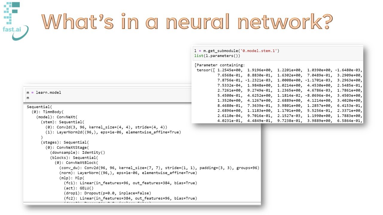
00:21:23.120 | So you can actually grab the trained model by just grabbing the dot model attribute

00:21:27.880 | So I'm just going to call that m and then if I type m I can look at the model and so here it is

00:21:33.580 | Lots of stuff. So what is this stuff? Well, we'll learn about it all over time, but basically what you'll find is

00:21:42.560 | It contains lots of layers because this is a deep learning model and you can see it's kind of like a tree

00:21:49.640 | That's because lots of the layers themselves consist of layers

00:21:52.760 | so there's a whole layer called the Tim body which is most of it and

00:21:59.560 | then right at the end there's a second layer called sequential and

00:22:02.960 | then the Tim body contains

00:22:05.920 | something called model and

00:22:08.080 | It can then it contains something called stem and something called stages and then stages can contain zero one two, etc

00:22:16.880 | So what is all this stuff? Well, let's take a look at one of them

00:22:20.520 | So to take a look at one of them, there's a really convenient

00:22:25.480 | Method in pytorch called get sub module where we can pass in a kind of a dotted string

00:22:33.240 | Navigating through this hierarchy. So zero model stem one goes zero model stem one

00:22:40.120 | So this is going to return this layer norm 2d thing. So what is this layer norm 2d thing?

00:22:46.700 | well, the key thing is

00:22:48.700 | It's got some code is with the mathematical function. We talked about and then the other thing that we learned about is it has

00:22:56.140 | Parameters and so we can list its parameters and look at this. It's just lots and lots and lots of numbers

00:23:01.500 | Let's grab another example. We could have a look at zero dot model dot stages dot zero blocks dot one dot MLP dot FC one and

00:23:09.820 | parameters

00:23:12.140 | another big bunch of numbers

00:23:14.420 | So what's going on here? What are these numbers and where at earth did they come from and how come these?

00:23:22.500 | Numbers can figure out whether something is a basset hound or not

00:23:26.420 | Okay, so

00:23:30.180 | To answer that question we're going to have a look at a

00:23:36.900 | Kaggle notebook

00:23:43.420 | How does a neural network really work

00:23:45.700 | But a local version of it here which I'm going to take you through and the basic idea is

00:23:52.540 | Machine learning models are things that fit

00:23:56.220 | Functions to data. So we start out with a very very flexible

00:24:00.620 | in fact an infinitely flexible as we've discussed function and your network and

00:24:04.740 | We get it to do a particular thing

00:24:07.460 | Which is to recognize the patterns in the data examples we give it

00:24:12.140 | so

00:24:14.060 | Let's do a much simpler example

00:24:16.060 | Than a neural network. Let's do a quadratic

00:24:20.280 | So let's create a function f which is 3x squared

00:24:24.340 | plus 2x

00:24:26.900 | Plus one. Okay, so it's a quadratic with coefficients 3 2 and 1

00:24:31.620 | So we can plot that function f and give it a title

00:24:35.140 | If you haven't seen this before things between dollar signs is what's called latex

00:24:39.580 | It's basically how we can create kind of typeset mathematical equations

00:24:42.920 | Okay, so let's run that

00:24:47.380 | And so here you can see the function here you can see the title I passed it and here is

00:24:54.680 | quadratic, okay, so what we're going to do is we're going to

00:24:58.860 | Imagine that we don't know that's the true

00:25:02.140 | Mathematical function we're trying to find as it's obviously much simpler than the function that figures out whether an image is a

00:25:09.100 | Basset hound or not that we're just going to start super simple

00:25:12.000 | So this is the real function and we're going to try to to recreate it from some data

00:25:17.340 | Now it's going to be very helpful if we have an easier way of creating different quadratics

00:25:25.380 | So I have to find a kind of a general form of a quadratic here

00:25:29.300 | If the with coefficients a b and c and at some particular point x it's going to be ax squared plus bx plus c

00:25:36.940 | And so let's test that

00:25:38.940 | Okay, so that's for x equals 1.5. That's 3x squared plus 2x plus 1 which is the quadratic we were did before

00:25:48.140 | Now we're going to want to create lots of different quadratics to test them out and find out which one's best

00:25:57.220 | so this is a

00:26:00.460 | Somewhat advanced but very very helpful feature of Python that's worth learning if you're not familiar with it

00:26:05.160 | And it's used in a lot of programming languages. It's called a partial application of a function. Basically. I want this exact function

00:26:11.340 | but I want to fix the values of a b and c to pick a particular quadratic and

00:26:17.060 | the way you fix the values of the function is you call this thing in Python called partial and you pass in the function and

00:26:24.580 | Then you pass in the values that you want to fix

00:26:27.020 | so for example

00:26:31.220 | If I now say make quadratic 3 2 1 that's going to create a quadratic equation with coefficients 3 2 and 1

00:26:40.200 | And you can see if I then pass in so that's now f if I pass in 1.5. I get the exact same value I did before

00:26:49.900 | Okay, so we've now got an ability to create any quadratic

00:26:56.420 | Equation we want by passing in the parameters of the coefficients of the quadratic

00:27:01.140 | That gives us a function that we can then just call as just like any normal function

00:27:05.660 | So that only needs one thing now, which is the value of x because the other three a b and c are now fixed

00:27:11.100 | So if we plot that function

00:27:15.540 | We'll get exactly the same shape because it's the same coefficients

00:27:19.940 | Okay

00:27:22.300 | so

00:27:23.460 | Now I'm going to show an example of of some data some data that

00:27:28.960 | Matches the shape of this function, but in real life data is never exactly going to match the shape of a function

00:27:36.620 | It's going to have some noise. So here's a couple of

00:27:40.980 | functions to add some noise

00:27:43.860 | So you can see I've still got the basic functional form here, but this data is a bit dotted around it

00:27:54.060 | The level to which you look at how I implemented these is entirely up to you

00:27:59.180 | It's not like super necessary, but it's all stuff which you know the kind of things we use quite a lot

00:28:05.020 | So this is to create normally distributed random numbers

00:28:08.100 | This is how we set the seed so that each time I run this I've got to get the same random numbers

00:28:14.540 | This one is actually particularly helpful this creates a

00:28:20.060 | tensor so in this case a vector that goes from negative to

00:28:24.220 | to two in

00:28:26.500 | Equal steps and there's 20 of them. That's why there's 20 steps along here

00:28:30.860 | So then my y values is just f of x

00:28:35.940 | With this amount of noise added

00:28:39.860 | Okay, so as I say the details of that don't matter too much. The main thing to know is we've got some

00:28:46.180 | Random data now and so this is the idea is now we're going to try to reconstruct the original

00:28:51.940 | Quadratic equation find one which

00:28:54.900 | matches this data

00:28:57.220 | So how would we do that?

00:28:59.220 | Well what we can do is we can create a function called plot quadratic

00:29:07.540 | That first of all plots our data as a scatter plot and then it plots a function which is a quadratic

00:29:15.060 | a quadratic we pass in

00:29:17.060 | Now that's a very helpful thing for experimenting

00:29:20.220 | In Jupiter notebooks, which is the at interact?

00:29:24.660 | Function if you add it on top of a function

00:29:28.620 | Then it gives you these nice little sliders

00:29:31.700 | So here's an example of a quadratic with coefficients 1.5 1.5 1.5

00:29:39.860 | And it doesn't fit particularly well

00:29:43.860 | So how would we try to make this fit better? Well, I think what I'd do is I'd take the first slider and

00:29:49.340 | I would try moving it to the left and see if it looks better or worse

00:29:52.700 | That looks worse to me I think it needs to be more curvy so let's try the other way

00:29:58.340 | Yeah, that doesn't look bad let's do the same thing for the next slider have it this way

00:30:04.860 | No, I think that's worse. Let's try the other way

00:30:08.620 | Okay final slider

00:30:11.660 | Try this way

00:30:13.700 | It's worse this way

00:30:15.700 | So you can see what we can do we can basically pick each of the coefficients

00:30:20.700 | One at a time try increasing a middle bit see if that improves it try decreasing it a little bit

00:30:26.380 | See if that improves it find the direction that improves it and then slide it in that direction a little bit

00:30:32.100 | and then when we're done we can go back to the first one and see if

00:30:34.820 | We can make it any better

00:30:38.140 | Now we've done that

00:30:41.500 | And actually you can see that's not bad because I know the answer is meant to be 3 2 1 so they're pretty close

00:30:47.260 | And I wasn't shooting I promise

00:30:50.100 | That's basically

00:30:53.900 | What we're going to do that's basically how those parameters

00:30:56.820 | Created but we obviously don't have time because the you know big fancy models have

00:31:03.700 | Often hundreds of millions of parameters. We don't have time to try a hundred hundred million sliders, so we did something better

00:31:11.580 | Well the first step is we need a better idea of like when I move it is it getting better or is it getting worse?

00:31:17.540 | So if you remember back to

00:31:20.620 | after Samuel's

00:31:23.860 | Description of machine learning that we learned about chapter one of the book and in lesson one

00:31:28.600 | We need some

00:31:32.020 | Something we can measure which is a number that tells us how good is our model and if we had that then as we move

00:31:38.580 | The sliders we could check to see whether it's getting better or worse

00:31:41.540 | So this is called a loss function

00:31:44.780 | So there's lots of different loss functions you can pick but perhaps the most simple and common is

00:31:49.780 | Mean squared error which is going to be so it's going to get in our predictions

00:31:54.940 | And it's got the actuals and we're going to go predictions minus actuals squared and take the mean

00:32:01.220 | So that's mean squared

00:32:03.740 | so

00:32:05.220 | If I now rerun the exact same thing I had before but this time I'm going to calculate the loss the MSE between

00:32:12.700 | The values that we predict f of x

00:32:15.940 | Remember where f is the quadratic we created and the actuals y and this time I'm going to add a title to our function

00:32:23.580 | Which is the loss?

00:32:26.020 | So now

00:32:29.820 | Let's do this more rigorously

00:32:32.500 | We're starting at a mean squared error of eleven point four six. So let's try moving this to the left and see if it gets better

00:32:38.100 | No, wait, so move it to the right

00:32:40.700 | All right, so around there, okay now let's try this one

00:32:47.500 | Okay best when I go to the right

00:32:54.980 | Okay, what about C 3.91? It's getting worse

00:33:00.820 | So I keep going

00:33:02.820 | So we're about there and so now we can repeat that process, right?

00:33:07.180 | So we've we've had each of a B and C move a little bit. Let's go back to a

00:33:11.340 | Can I get any better than 3.28? Let's try moving left

00:33:14.900 | Yeah, that was a bit better and for B. Let's try moving left

00:33:19.420 | worse

00:33:22.300 | right was better and

00:33:24.300 | Have it finally see move to the right

00:33:27.580 | Oh

00:33:29.580 | Definitely better

00:33:32.940 | There we go

00:33:35.580 | Okay, so

00:33:37.460 | That's a more rigorous approach

00:33:39.460 | It's still manual

00:33:41.020 | But at least we can like we don't have to rely on us to kind of recognize does it look better or worse?

00:33:46.100 | So finally we're going to automate this

00:33:49.940 | So the key thing we need to know is for each parameter

00:33:56.060 | When we move it up

00:33:58.060 | Does the loss get better or when we move it down? Does the loss get better?

00:34:03.060 | One approach would be to try right?

00:34:07.300 | We could manually increase the parameter a bit and see if the loss improves and vice versa

00:34:12.580 | But there's a much faster way

00:34:15.260 | And the much faster way is to calculate its derivative

00:34:18.460 | So if you've forgotten what a derivative is, no problem. There's lots of tutorials out there

00:34:24.140 | You could go to Khan Academy or something like that

00:34:25.900 | But in short the derivative is what I just said the derivative is a function that tells you

00:34:32.060 | If you increase the input does the output increase or decrease and by how much so that's called the slope

00:34:39.660 | or the gradient

00:34:42.220 | now the good news is

00:34:44.420 | Pytorch can automatically calculate that for you. So if you

00:34:48.340 | went through

00:34:51.180 | Horrifying months of learning derivative rules in year 11 and worried you're going to have to remember them all again. Don't worry you don't

00:34:58.140 | You don't have to calculate any of this yourself. It's all done for you. Watch this

00:35:02.940 | So the first thing to do is we need a function that takes the coefficients of the quadratic a b and c as inputs I

00:35:11.540 | Put them all on the list. You'll see why in a moment. I kind of call them parameters

00:35:16.700 | We create a quadratic

00:35:20.300 | passing in those parameters a b and c

00:35:22.420 | This star on the front is a very very common thing in Python

00:35:26.460 | Basically, it takes these parameters and spreads them out to turn them into a b and c and pass each of them to the function

00:35:34.180 | So we've now got a quadratic

00:35:36.180 | with those coefficients

00:35:38.820 | And then we return the mean squared error of our predictions against our actions

00:35:45.100 | So this is a function that's going to take the coefficients of a quadratic and return the loss

00:35:50.180 | So let's try it

00:35:54.260 | Okay, so if we start with a b and c at 1.5 we get a mean squared error of 11.46

00:36:02.540 | It looks a bit weird it says it's a tensor

00:36:06.380 | So don't worry about that too much in short in Pytorch

00:36:13.020 | Everything is a tensor a tensor just means that you don't it doesn't just work with numbers

00:36:17.700 | It also works with lists or vectors of numbers. That's got a 1d tensor

00:36:22.580 | Rectangles of numbers so tables of numbers. It's got a 2d tensor

00:36:27.380 | Layers of tables of numbers that's got a 3d tensor and so forth. So in this case, this is a single number

00:36:34.580 | But it's still a tensor. That means it's just wrapped up in the Pytorch

00:36:40.540 | Machinery that allows it to do things like calculate derivatives, but it's still just the number 11.46

00:36:46.340 | All right, so what I'm going to do is I'm going to create my parameters a b and c and I'm going to put them all in

00:36:55.220 | A single 1d tensor a 1d tensor is also known as a rank 1 tensor

00:37:00.900 | So this is a rank

00:37:03.540 | 1 tensor and it contains the list of numbers 1.5 1.5 1.5

00:37:10.180 | And then I'm going to tell Pytorch

00:37:12.780 | That I want you to calculate the gradient

00:37:15.860 | For these numbers whenever we use them in a calculation and the way we do that is we just say requires credit

00:37:22.740 | So here is our

00:37:26.180 | Tensor it contains 1.5 3 times and it also tells us it's we flagged it to say please calculate gradients for this

00:37:34.260 | particular tensor when we use it in calculations

00:37:38.700 | So let's now use it in the calculation. We're going to pass it to that quad MSC. That's the function

00:37:45.060 | We just created that gets the MSC a mean squared error for a set of coefficients

00:37:49.780 | And not surprisingly, it's the same number we saw before 11.46. Okay

00:37:55.820 | Not very exciting

00:37:57.900 | But there is one thing that's very exciting which is added an extra thing to the end called grad function

00:38:02.820 | And this is the thing that tells us that if we wanted to

00:38:06.840 | Pytorch knows how to create calculate the gradients

00:38:10.460 | For our inputs and to tell Pytorch just please go ahead and do that calculation

00:38:16.340 | You call backward on the result of your loss function. Now when I run it nothing happens

00:38:24.260 | It doesn't look like anything happens. But what does happen is it's just added an attribute called grad

00:38:30.780 | Which is the gradient to our inputs ABC. So if we run this cell

00:38:34.020 | This tells me that if I increase a the loss will go down

00:38:40.940 | If I increase B, the loss will go down a bit less

00:38:45.580 | You know if I increase C, the loss will go down

00:38:49.260 | Now we want the loss to go down

00:38:51.980 | Right. So that means we should increase a B and C

00:38:56.700 | Well, how much by well given that a is says if you increase a even a little bit the loss

00:39:03.180 | Improves a lot that suggests we're a long way away from the right answer. So we should probably increase this one a lot

00:39:08.980 | This one the second most and this one the third most

00:39:12.380 | So this is saying when I increase

00:39:15.220 | This parameter the loss decreases. So in other words, we want to adjust our parameters a B and C

00:39:23.500 | By the negative of these we want to increase increase increase

00:39:27.860 | So we can do that

00:39:30.660 | By saying, okay, let's take our ABC

00:39:33.340 | Minus equals so that means equals ABC minus

00:39:38.380 | the gradient

00:39:41.540 | But we're just going to like decrease it a bit. We don't want to jump too far. Okay, so just we're just going to go

00:39:46.460 | A small distance. So we're going to we're just going to somewhat arbitrarily pick point. Oh one

00:39:52.620 | So that is now going to create a new set of parameters

00:39:55.940 | Which are going to be a little bit bigger than before because we subtracted negative numbers

00:40:00.380 | And we can now calculate the loss again

00:40:03.820 | so remember before

00:40:06.500 | It was eleven point four six

00:40:08.780 | So hopefully it's going to get better

00:40:11.300 | Yes, it did

00:40:13.100 | ten point one one

00:40:15.100 | There's one extra line of code which we didn't mention which is with torch dot no grad

00:40:21.340 | Remember earlier on we said that the parameter ABC requires grad and that means pytorch will automatically calculate

00:40:28.380 | Its derivative when it's used in a in a function

00:40:32.380 | Here it's being used in a function, but we don't want the derivative of this. This is not our loss

00:40:37.900 | Right. This is us updating the gradients. So this is basically

00:40:42.020 | the standard in a part of a pytorch loop and every neural net deep learning machine pretty much every machine learning model

00:40:51.340 | At least of this style that your build basically looks like this

00:40:55.020 | If you look deep inside fast.io source code, you'll see something that basically looks like this

00:41:00.460 | So we could automate that right? So let's just take those steps which is we're going to

00:41:10.540 | Calculate let's go back to here. We're going to calculate the mean squared error for our quadratic

00:41:20.340 | Call backward and then subtract the gradient times a small number from the gradient

00:41:27.260 | Let's do it five times

00:41:30.380 | So so far we're up to a loss of ten point one

00:41:32.700 | So we're going to calculate our loss call dot backward to calculate the gradients

00:41:38.100 | and then with no grad

00:41:41.100 | subtract the gradients times a small number and print how we're going and

00:41:49.020 | There we go. The loss keeps improving

00:41:52.300 | So we now have

00:41:56.060 | Some coefficients

00:42:07.060 | And

00:42:09.500 | There they are three point two one point nine two point. Oh, so they're definitely heading in the right direction

00:42:15.980 | So

00:42:17.980 | That's basically how we do it's called optimization

00:42:23.500 | Okay, so you'll hear a lot in deep learning about optimizers. This is the most basic kind of

00:42:29.420 | Optimizer, but they're all built on this principle of course

00:42:33.380 | It's called gradient descent and you can see why it's called gradient descent. We calculate the gradients and

00:42:38.980 | Then do a descent which is we're trying to decrease the loss

00:42:45.500 | so

00:42:47.380 | Believe it or not. That's that's

00:42:49.380 | The entire foundations of how we create those parameters. So we need one more piece

00:42:55.900 | Which is what is the mathematical function that we're finding parameters for?

00:42:59.940 | We can't just use quadratics, right because it's pretty unlikely that the relationship between

00:43:06.460 | parameters and

00:43:08.420 | Whether a pixel is part of a basset hound is a quadratic. It's going to be something much more complicated

00:43:13.500 | No problem

00:43:15.500 | It turns out that

00:43:20.620 | We can create an infinitely flexible function from this one tiny thing

00:43:26.100 | This is called a rectified linear unit

00:43:30.160 | The first piece I'm sure you will recognize

00:43:33.020 | It's a linear function. We've got our output Y

00:43:36.900 | our input X and

00:43:40.140 | coefficients M and B. This is even simpler than our quadratic and

00:43:45.140 | This is a line

00:43:48.460 | And torch.clip is a function that takes the output Y and if it's greater than that number

00:43:56.340 | It turns it into that number. So in other words, this is going to take anything that's negative and make it zero

00:44:01.660 | So this function is going to do two things

00:44:06.820 | Calculate the output of a line and if it is bigger than or smaller than zero, it'll make it zero

00:44:12.180 | So that's rectified linear

00:44:15.620 | So let's use partial

00:44:18.180 | To take that function and set the M and B to one and one. So this is now going to be this function here

00:44:24.420 | will be

00:44:26.740 | Y equals X plus one followed by this torch.clip

00:44:30.740 | And here's the shape okay as we'd expect it's a line

00:44:37.340 | Until it gets under zero

00:44:39.340 | When it comes to the line, it becomes a horizontal line

00:44:43.500 | So we can now do the same thing we can take this plot function and make it interactive

00:44:50.140 | using interact and

00:44:53.020 | We can see what happens when we change these two parameters M and B. So we're now plotting

00:44:58.460 | the rectified linear and fixing M and B

00:45:01.260 | So M is the slope

00:45:04.180 | And B is the intercept for the shift up and down

00:45:14.340 | Okay

00:45:17.380 | so that's

00:45:18.900 | how those

00:45:20.300 | Work now, why is this interesting? Well, it's not interesting of itself

00:45:24.700 | but what we could do is we could take this rectified linear function and

00:45:30.300 | create a double value

00:45:33.580 | Which adds up to rectified linear functions together

00:45:37.540 | So there's some slope M1B1, some second slope N2B2. We're going to calculate it at some point X and

00:45:45.820 | So let's take a look

00:45:49.540 | at what that function looks like if we plot it and

00:45:53.020 | You can see what happens is we get this downward slope and then a hook and then an upward slope

00:45:58.700 | So if I change M1, it's going to change the slope of that first bit

00:46:03.260 | and

00:46:04.420 | B1 is going to change its position

00:46:06.420 | Okay, and I'm sure you won't be surprised to hear that M2 changes the slope of the second bit and

00:46:13.700 | B2

00:46:16.660 | changes that location

00:46:18.660 | Now this is interesting. Why?

00:46:23.220 | Because we don't just have to do a double value

00:46:26.380 | We could add as many values together as we want

00:46:30.780 | And if we add as many values together as we want, then we can have an arbitrarily squiggly function and with enough values

00:46:39.020 | We can match it as close as we want

00:46:42.300 | right, so you could imagine incredibly squiggly like I don't know like an audio waveform of me speaking and

00:46:48.860 | If I gave you a hundred million values together, you could almost exactly match that

00:46:58.540 | Now we want

00:47:00.540 | functions that are not just

00:47:02.540 | That we've put in 2D

00:47:04.660 | We want things that can have more than one input

00:47:06.660 | but you can add these together across as many dimensions as you like and so exactly the same thing will give you a

00:47:12.540 | value over surfaces or

00:47:15.420 | a value over

00:47:18.140 | 3D, 4D, 5D and so forth and it's the same idea with this

00:47:23.340 | incredibly simple foundation

00:47:26.860 | You can construct an

00:47:28.860 | arbitrarily

00:47:31.220 | accurate precise

00:47:33.220 | model

00:47:35.500 | Problem is you need some numbers for them, you need parameters. Oh, no problem. We know how to get parameters

00:47:46.220 | We use gradient descent

00:47:48.860 | So believe it or not

00:47:51.740 | We have just derived

00:47:55.260 | big money

00:47:57.020 | everything from now on is

00:47:59.020 | Tweaks to make it faster and make it need less data

00:48:05.220 | You know, this is this is it

00:48:10.500 | Now I remember a few years ago when I said something like this in a class

00:48:15.300 | Somebody on the forum was like this reminds me of that thing about how to draw an owl

00:48:19.260 | Jeremy is basically saying okay step one

00:48:22.140 | draw two circles

00:48:24.820 | step two, draw the rest of the owl

00:48:26.820 | The thing I find I have a lot of trouble explaining to students is when it comes to deep learning

00:48:33.420 | there's nothing between these two steps. When you have

00:48:35.880 | values getting added together and

00:48:38.860 | gradient descent to optimize the parameters and

00:48:42.220 | samples of inputs and outputs that you want

00:48:45.300 | The computer draws the owl, right? That's it

00:48:51.780 | So we're going to learn about all these other tweaks and they're all very important

00:48:55.500 | But when you come down to like trying to understand something in deep learning, just try to keep coming back to remind yourself

00:49:02.780 | of what it's doing

00:49:05.940 | Which it's using gradient descent to set some parameters to make a wiggly function

00:49:11.100 | Which is basically the addition of lots of rectified linear units or something very similar to that

00:49:15.580 | match your data

00:49:18.340 | Okay, so we've got some questions on the forum

00:49:24.660 | Okay, so question from Zakiya with six upvotes so for those of you

00:49:33.060 | watching the video what we do in the lesson is we want to make sure that the

00:49:37.740 | Questions that you hear answered are the ones that people really care about

00:49:41.040 | So we pick the ones which get the most upvotes. This question is

00:49:46.940 | Is there perhaps a way to try out all the different models and automatically find the best performing one?

00:49:53.220 | Yes, absolutely you can do that so

00:49:59.820 | If we go back to our training script remember there's this thing called list models and

00:50:08.340 | It's a list of strings. So you can easily add a for loop around this

00:50:13.460 | that basically goes you know for

00:50:16.340 | Architecture in Tim dot list models and you could do the whole lot which would be like that and then you could

00:50:25.980 | Do that and away you go

00:50:30.580 | It's going to take a long time for 500 and something models

00:50:34.580 | So generally speaking like I've I've never done anything like that myself

00:50:40.100 | I would rather look at a picture like this and say like okay. Where am I in?

00:50:44.700 | the vast majority of the time this is something this would be the biggest I reckon number one mistake of

00:50:51.100 | Beginners I see is that they jump to these models

00:50:55.540 | From the start of a new project at the start of a new project. I pretty much only use ResNet 18

00:51:01.740 | Because I want to spend all of my time

00:51:06.220 | Trying things out and I try different data augmentation. I'm going to try different ways of cleaning the data

00:51:10.940 | I'm going to try

00:51:13.980 | you know

00:51:16.420 | Different external data I can bring in and so I want to be trying lots of things now

00:51:22.180 | I want to be able to try it as fast as possible, right? So

00:51:25.300 | Trying better architectures is the very last thing that I do and

00:51:33.980 | What I do is once I've spent all this time, and I've got to the point where I've got okay

00:51:37.620 | I've got my ResNet 18 or maybe you know ResNet 34 because it's nearly as fast

00:51:41.700 | And

00:51:44.980 | I'm like okay. Well. How accurate is it?

00:51:46.980 | How fast is it?

00:51:49.540 | Do I need it more accurate for what I'm doing do I need it faster for what I'm doing?

00:51:54.980 | Could I accept some trade-off to make it a bit slower to make more accurate and so then I'll have a look and I'll say

00:52:00.260 | Okay, well I kind of need to be somewhere around 0.001 seconds, and so I try a few of these

00:52:04.980 | So that would be how I would think about that

00:52:09.860 | Okay next question from the forum is around how do I know if I have enough data?

00:52:18.300 | What are some signs that indicate my problem needs more data?

00:52:22.780 | I think it's pretty similar to the architecture question, so you've got something out of data

00:52:30.640 | Presumably you've you know you've started using all the data that you have access to you built your model

00:52:36.240 | You've done your best

00:52:38.760 | Is it good enough?

00:52:41.360 | Do you have the accuracy that you need for whatever it is you're doing?

00:52:45.840 | You can't know until you've trained the model, but as you've seen it only takes a few minutes to train a quick model

00:52:54.780 | so

00:52:57.280 | my very strong opinion is that the vast majority of

00:53:00.560 | Projects I see in industry wait far too long before they train their first model

00:53:06.840 | You know my opinion you want to train your first model on day one with whatever

00:53:11.720 | CSV files or whatever that you can hack together

00:53:15.080 | And you might be surprised that none of the fancy stuff

00:53:19.960 | You're thinking of doing is necessary because you already have a good enough accuracy for what you need

00:53:24.200 | Or you might find quite the opposite you might find that oh my god with we're basically getting no accuracy at all

00:53:30.400 | Maybe it's impossible

00:53:32.600 | These are things you want to know at the start

00:53:35.440 | Not at the end

00:53:38.040 | We'll learn lots of techniques both in this part of the course and in part two

00:53:42.360 | About ways to really get the most out of your data

00:53:45.560 | In particular there's a reasonably recent technique called semi-supervised learning

00:53:51.880 | Which actually lets you get dramatically more out of your data

00:53:54.640 | And we've also started talking already about data augmentation, which is a classic technique you can use

00:54:00.040 | So you generally speaking it depends how expensive is it going to be to get more data?

00:54:03.960 | But also what do you mean when you say get more data? Do you mean more labeled data?

00:54:08.000 | Often it's easy to get lots of inputs and hard to get lots of outputs

00:54:13.040 | For example in medical imaging where I've spent a lot of time

00:54:16.720 | It's generally super easy to jump into the radiology archive and grab more CT scans

00:54:22.240 | But it's maybe very difficult and expensive to

00:54:25.880 | You know draw segmentation masks and and pixel boundaries and so forth on them

00:54:31.760 | So often you can get more

00:54:35.880 | You know in this case images

00:54:39.160 | Or text or whatever and maybe it's harder to get labels

00:54:43.600 | And again, there's a lot of stuff you can do using stuff things like we'll discuss semi-supervised learning to actually take advantage of unlabeled data

00:54:50.720 | as well

00:54:53.200 | Okay

00:54:56.600 | Final question here in the quadratic example where we calculated the initial derivatives for A B and C

00:55:02.800 | We got values of minus 10.8 minus 2.4, etc. What unit are these expressed in?

00:55:08.440 | Why don't we adjust our parameters by these values themselves?

00:55:11.520 | So I guess the question here is why are we multiplying it by a small number?

00:55:14.400 | Which in this case is 0.01?

00:55:17.560 | Okay, let's take those two parts of the question

00:55:20.560 | What's the unit here

00:55:27.560 | the unit is

00:55:29.560 | for each increase in x of 1

00:55:32.720 | how much does what sorry in for each increase in in a of 1 so if I increase a from

00:55:41.360 | this case

00:55:42.840 | We have 1.5. So if we increase from 1.5 to 2.5

00:55:46.720 | What would happen to the loss?

00:55:49.480 | And the answer is it would go down by 10.9

00:55:52.180 | 887 now, that's not exactly right because it's kind of like

00:55:58.280 | It's kind of like in an infinitely small space right because actually it's going to be curved

00:56:04.600 | Right, but if it if it stays its data, that's like that's what would happen

00:56:10.280 | so if we

00:56:11.720 | increased B by 1

00:56:13.720 | The loss would decrease if it stayed constant

00:56:17.800 | You know if the slope stayed the same the loss would decrease by minus 2.1 to 2

00:56:22.320 | Okay, so why would we not just

00:56:26.760 | Change it directly by these numbers. Well, the reason is

00:56:32.920 | The reason is that if we

00:56:37.960 | have some function that we're fitting

00:56:47.960 | And there's some kind of interesting theory that says that once you get close enough to the

00:56:57.280 | Optimal value all functions look like quadratics anyway, right? So we can kind of safely draw it in this kind of shape

00:57:06.080 | Because this is what they end up looking like if you get close enough

00:57:08.480 | And we're like, let's say we're way out

00:57:11.800 | Over here. Okay, so we were measuring I

00:57:16.320 | Used my daughter's favorite pens and I sparkly ones. So we're measuring the slope here

00:57:22.960 | There's a very steep slope

00:57:26.720 | So that seems to suggest we should jump a really long way. So we jump a really long way

00:57:34.800 | And what happened? Well, we jumped way too far. And the reason is that that slope

00:57:40.560 | decreased as

00:57:42.960 | We moved a lot and so that's generally what's going to happen, right?

00:57:47.320 | Particularly as you approach the optimal is generally the slopes going to decrease

00:57:51.080 | So that's why we multiply the gradient by a small number

00:57:55.040 | And that small number is a very very very important number. It has a special name

00:58:02.800 | It's called the learning rate

00:58:05.280 | And this is an example of a

00:58:11.520 | Hyper parameter, it's not a parameter. It's not one of the actual coefficients of your function

00:58:17.720 | But it's a parameter you use to calculate the parameters

00:58:22.000 | Pretty better, right? It's a hyper parameter. And so it's something you have to pick now. We haven't picked any yet

00:58:30.760 | In any of the stuff we've done that I remember and that's because fast AI generally picks reasonable defaults

00:58:36.720 | For most things but later in the course we will learn about how to try and find

00:58:41.360 | really good

00:58:43.800 | Learning rates and you will find sometimes you need to actually spend some time finding a good learning rate

00:58:49.960 | You could probably understand the intuition here if you pick a learning rate, that's too big

00:58:55.200 | You'll jump too far

00:58:57.720 | And so you'll end up

00:59:00.280 | way over here and then you will try to

00:59:03.600 | Then jump back again and you'll jump too far the other way and you'll actually

00:59:08.480 | Diverge and so if you ever see when your model is training, it's getting worse and worse

00:59:13.560 | Probably means your learning rates too big

00:59:16.440 | What would happen on the other hand if you pick a learning rate that's too small?

00:59:20.920 | Then you're going to

00:59:25.480 | Take tiny steps and of course the flatter it gets the smaller the steps are going to get and

00:59:31.440 | So you're going to get very very bored

00:59:34.040 | So finding the right learning rate is a compromise

00:59:37.560 | Between the speed at which you find the answer and the possibility that you're actually going to shoot past it and get worse and worse

00:59:43.800 | Okay, so one of the bits of feedback I got quite a lot in the survey is that people want a break halfway through

00:59:52.720 | Which I think is a good idea. So I think now is a good time to have a break

00:59:55.520 | So let's come back in 10 minutes at 25 past 7

01:00:00.160 | Okay, hope you had a good rest have a good break I should say

01:00:17.760 | So I want to now show you a really really important

01:00:22.280 | mathematical

01:00:24.040 | computational trick

01:00:26.040 | Which is we want to do a whole bunch of?

01:00:28.440 | values

01:00:31.680 | All right, so we're going to be wanting to do a whole lot of

01:00:36.800 | MX plus base and we want don't just want to do MX plus B. We're going to want to have like lots of

01:00:44.000 | Variables so for example every single pixel of an image would be a separate variable

01:00:49.800 | so we're going to multiply every single one of those times some coefficient and then add them all together and

01:00:55.720 | then do the

01:00:58.920 | The crop the the ReLU and then we're going to do it a second time with a second bunch of parameters

01:01:05.000 | And then a third time and a fourth time and fifth time

01:01:07.120 | It's going to be pretty inconvenient to write out a hundred million ReLU's

01:01:13.920 | But so happens there's a mathematical single mathematical operation that does all of those things for us except for the final replace

01:01:21.840 | negatives with zeros and it's called matrix multiplication I

01:01:25.400 | Expect everybody at some point did matrix multiplication at high school. I suspect also a lot of you have forgotten works

01:01:32.920 | when people talk about linear algebra in

01:01:36.440 | deep learning

01:01:39.520 | They give the impression you need years of graduate school study to learn all this linear algebra

01:01:45.280 | You don't actually all you need almost all the time is matrix multiplication and it couldn't be simpler

01:01:52.800 | I'm going to show you a couple of different ways

01:01:54.000 | The first is there's a really cool site called matrix multiplication dot XYZ you can put in any matrix you want

01:02:00.320 | So I'm going to put in

01:02:03.640 | This one

01:02:07.360 | So this matrix is saying I've got three rows of data

01:02:10.840 | with three

01:02:13.480 | variables

01:02:14.440 | So maybe they're tiny to the tiny images with three pixels and the value of the first one is 1 2 1

01:02:21.160 | The second is 0 1 1 and the third is 2 3 1

01:02:24.520 | So those are our three rows of data

01:02:27.520 | These are our three sets of coefficients. So we've got a

01:02:31.960 | B and C in our data. So so I guess you'd call it x1 x2 and x3 and then here's our first set of coefficients a B and C

01:02:39.560 | 2 6 and 1

01:02:42.160 | And then our second set is 5 7 and 8

01:02:44.640 | So here's what happens when we do matrix multiplication that second this matrix here of coefficients

01:02:51.440 | gets flipped around

01:02:54.480 | And

01:02:56.840 | we do

01:02:58.640 | This is the multiplications and additions that I mentioned right? So multiply and multiply add multiply add so that's going to give you

01:03:06.440 | the first number

01:03:09.040 | because that is the

01:03:11.160 | left hand column of the

01:03:13.200 | Second matrix times the first row so that gives you the top left

01:03:18.640 | result

01:03:21.120 | So the next one is going to give us two results, right?

01:03:23.920 | So we've got now the right hand one with the top row and the left hand one with the second row

01:03:28.960 | Keep going down

01:03:32.360 | Go down

01:03:34.400 | And that's it that's what matrix multiplication is it's multiplying things together and adding them up

01:03:40.840 | So there'd be one more step to do to make this a layer of a neural network

01:03:45.200 | Which is if this had any negatives we replace them with zeros

01:03:48.300 | that's my matrix multiplication is

01:03:52.600 | the

01:03:54.080 | critical

01:03:55.880 | Foundation or mathematical operation and basically all of deep learning

01:03:59.560 | so the

01:04:02.360 | GPUs that we use the thing that they are good at is this matrix multiplication

01:04:08.520 | They have special cores called tensor cores

01:04:11.560 | Which we can basically only do one thing which is to multiply together two four by four matrices

01:04:18.400 | And then they do that lots of times with bigger matrices

01:04:22.600 | so I'm going to show you an

01:04:24.600 | example of this we're actually going to build a

01:04:27.480 | complete machine learning model on real data in the spreadsheet

01:04:33.720 | So

01:04:40.000 | Fast AI has become kind of famous for a number of things and one of them is using spreadsheets

01:04:44.880 | To create deep learning models. We haven't done it for a couple of years. I'm pretty pumped to show this to you

01:04:51.240 | What I've done is I went over to cable

01:04:56.480 | Where there's a competition I actually helped create many years ago called Titanic

01:05:05.920 | And it's like an ongoing competition. So 14,000 people have entered it. So 12 teams have entered it so far

01:05:12.880 | It's just a competition for a bit of fun

01:05:15.960 | There's no end date and the data for it is the data about

01:05:20.880 | Who

01:05:25.680 | Who survived and who didn't

01:05:29.000 | from the real Titanic disaster

01:05:32.440 | And so I clicked here on the download button to grab it on my computer that gave me a CSV

01:05:38.320 | Which I opened up in Excel

01:05:43.520 | The first thing I did then was I just removed a few columns that

01:05:46.840 | Clearly were not going to be important things like the name of the passengers the passenger ID

01:05:51.960 | just try to make it a bit simpler and

01:05:55.000 | so I've ended up with

01:05:57.400 | Each row of this is one passenger. The first column is the dependent variable. The dependent variable is the thing we're trying to predict

01:06:04.160 | did they survive and

01:06:07.280 | The remaining are some information such as what class of the boat first second or third class for sex their age

01:06:14.160 | How many siblings in the family?

01:06:16.680 | So you should always look for a data dictionary to find out what's what number of parents and children, okay

01:06:31.040 | What was their fare and which of the three cities did they embark on? Okay, so there's that data

01:06:38.360 | Now when I first grabbed it I noticed that

01:06:44.120 | There were some people with no age now

01:06:48.140 | There's all kinds of things we could do for that. But for this purpose, I just decided to remove them and

01:06:57.400 | I found the same thing for embarked. I removed the blanks as well

01:07:00.900 | But that left me with nearly all of the data, okay, so then I've put that over here

01:07:08.220 | Here's our data with those rows removed

01:07:11.920 | Okay, that's the so this these are the columns that came directly from Kaggle

01:07:26.000 | So basically what we now want to do is we want to multiply each of these by a coefficient

01:07:30.560 | How do you multiply the word male?

01:07:33.520 | by a coefficient and

01:07:36.160 | How do you multiply s?

01:07:38.560 | coefficient

01:07:41.040 | You can't so I converted all of these two numbers male and female are very easy

01:07:45.960 | I created a column called is male and as you can see, there's just an if statement that says if sex is male

01:07:52.840 | That's one. Otherwise, it's zero

01:07:55.320 | And we can do something very similar for them, but we can have one column called did they embark in Southampton?

01:08:00.820 | Same deal and another column for today. What's the court shows boom?

01:08:06.080 | Sure, but did they embark in Cherberg?

01:08:09.760 | And their P class is one two or three which is a number but it's not really

01:08:17.180 | It's not really a continuous measurement of something. There isn't one or two or three things that different

01:08:24.760 | Levels, so I decided to turn those into similar things into these binary. They quote. These are called binary categorical variables

01:08:31.120 | So are they first class and?

01:08:33.920 | Are they second class?

01:08:36.840 | Okay, so that's all that

01:08:39.920 | The other thing that I was thinking well, you know that I kind of tried it and checked out what happened and what happened was

01:08:47.200 | the people with

01:08:49.960 | So I created some random numbers. So to create the random numbers

01:08:54.200 | I just went

01:08:56.120 | equals Rand

01:08:57.960 | Right and I copied those to the right and then I just went copy and I went paste values

01:09:04.240 | So that gave me some random numbers and that's my like so just because like I was like before I said all a B and C

01:09:10.800 | Let's just start them at 1.5 1.5 1.5 what we do in real life is we start our parameters at random numbers

01:09:17.280 | That are a bit more or a bit less than 0

01:09:20.880 | So these are random numbers

01:09:22.880 | Actually, sorry, I slightly lied. I didn't use Rand. I used Rand minus 0.5

01:09:28.160 | And that way I've got small numbers that were on either side of 0

01:09:32.240 | So then when I took each of these and I multiplied them by

01:09:39.760 | Fairs and ages and so forth what happened was that these numbers here

01:09:49.600 | Way bigger than

01:09:51.600 | You know these numbers here and so in the end all that mattered was what was their fair?

01:09:57.680 | That because they were just bigger than everything else

01:10:00.240 | So I wanted everything to basically go from 0 to 1 these numbers were too big

01:10:05.200 | So what I did up here is I just grabbed the maximum

01:10:08.040 | of this column the maximum of all the fairs is 512 and so then

01:10:16.000 | Actually, I do age first. I did a maximum of age because a similar thing, right? There's 80 year olds and there's two year olds and

01:10:22.360 | So then I'm over here. I just did okay. Well, what's their age?

01:10:26.880 | Divided by the maximum and so that way all of these are between 0 and 1

01:10:32.640 | Just like all of these are between 0 and 1

01:10:35.200 | So that's how I fix this is called normalizing the data

01:10:41.720 | Now we haven't done any of these things when we've done stuff with fast AI

01:10:47.720 | That's because fast AI does all of these things for you

01:10:50.800 | And we'll learn about how right?

01:10:54.000 | But it's all these things are being done behind the scenes

01:10:59.080 | The fair I did something a bit more which is I noticed there's some lots of very small fairs and

01:11:07.760 | There's also some a few very big fairs so like $70 and then $7 $7

01:11:13.000 | Generally speaking when you have lots of really big numbers and a few small ones

01:11:17.880 | So generally speaking when you've got a few really big numbers and lots of really small numbers. This is really common with with

01:11:25.640 | With money, you know because money kind of follows this relationship where a few people have lots of it

01:11:31.600 | And they spend huge amounts of it and most people don't have heaps

01:11:34.840 | If you take the log of something that's like that has that kind of extreme distribution

01:11:39.440 | You end up with something that's much more evenly distributed. So I've added this here called log fair

01:11:45.960 | as you can see

01:11:48.320 | And these are all around one which isn't bad. I could have normalized that as well

01:11:51.760 | But I was too lazy. I didn't bother because it seemed okay

01:11:54.520 | So at this point you can now see that if we start from here

01:12:02.680 | All of these are all around the same kind of level, right? So none of these columns are going to

01:12:08.240 | saturate the others

01:12:11.640 | So now I've got my coefficients which are just as I said, they're just random

01:12:17.680 | And so now I need to basically calculate

01:12:21.960 | Ax1 plus Bx2 plus Cx3 plus blah blah blah blah blah blah blah. Okay, and so to do that

01:12:31.000 | You

01:12:32.980 | Can use some product in Excel? I could have typed it out by hand. It'd be very boring

01:12:37.280 | But some product is just going to multiply each of these

01:12:40.920 | This one will be multiplied by

01:12:44.480 | There is it subset by this one

01:12:48.320 | This one will be multiplied by this one so forth and then they get all added together

01:12:52.580 | Now one thing if you're eagle-eyed you might be wondering is in a linear equation

01:12:59.440 | We have y equals mx plus B at the end

01:13:02.520 | There's this constant term and I do not have any constant term

01:13:06.320 | I've got something here called const, but I don't have any plus at the end

01:13:10.280 | How do we how's that working?

01:13:13.320 | Well, there's a nice trick that we pretty much always use in machine learning

01:13:17.360 | Which is to add a column of data just containing the number one every time

01:13:23.120 | If you have a column of data containing the number one every time and that parameter becomes your constant term

01:13:29.440 | So you don't have to have a special

01:13:31.660 | Constant term and so it makes out

01:13:34.600 | Code a little bit simpler when you do it that way. It's just a trick but everybody does it

01:13:41.160 | Okay, so this is now the result of our linear model

01:13:45.460 | So this is not I'm not even going to do value right? I'm just going to do

01:13:49.320 | the plane

01:13:52.280 | regression, right

01:13:54.200 | Now if you've done regression before you might have learned about it as something you kind of solve with various matrix things

01:14:00.400 | But in fact, you can solve a regression using gradient descent

01:14:05.040 | So I've just kind of had and created a loss for each row. And so the loss is going to be equal to

01:14:10.560 | Our prediction minus whether they survived

01:14:17.360 | squared so this is going to be our

01:14:21.520 | squared error

01:14:23.280 | And there they all are squared errors. And so here I've just

01:14:26.280 | Sum them up. I could have taken the mean. I guess that would have been a bit easier to think about

01:14:32.000 | But some is going to be give us the same result. So here's our loss

01:14:35.140 | And so now we need to optimize that using gradient descent

01:14:40.480 | So Microsoft Excel has a gradient descent optimizer in it called solver

01:14:45.920 | So I'll click solver and it'll say okay, what are you trying to optimize? It's this one here and I'm going to do it by changing

01:14:53.680 | These cells here

01:14:57.840 | And

01:15:00.200 | I'm trying to minimize it. And so we're starting a loss of 55.78

01:15:06.040 | Actually, let's change it to mean as well

01:15:12.320 | The word mean or average average

01:15:15.760 | All right, so start at 1.03

01:15:23.040 | So optimize that

01:15:30.640 | And there we go, so it's gone from 1.03 to 0.1 and so we can check the predictions so the first one

01:15:40.560 | It predicted exactly correctly

01:15:42.560 | It was they didn't survive and we predict wouldn't survive

01:15:47.120 | Ditto for this one

01:15:49.840 | It's very close and you can start to see

01:15:52.800 | So this one you can start to see a few issues here, which is like sometimes it's predicting less than one

01:15:58.080 | So it's less than zero and sometimes it's predicting more than one

01:16:01.280 | wouldn't it be cool if we had some way of

01:16:04.720 | Wouldn't it be cool if we had some way of constraining it to between zero and one and that's an example of some of the things

01:16:10.240 | We're going to learn about that make this stuff work a little bit better, right?

01:16:13.240 | But you can see it's doing an okay job. So this is not deep learning

01:16:16.160 | This is not a neural net yet. This is just a regression

01:16:18.640 | So to make it into a neural net

01:16:21.640 | We need to do it multiple times

01:16:24.480 | So I'm just going to do it twice. So now rather than one set of coefficients

01:16:29.280 | I've got two sets and again, I just put in random numbers

01:16:33.840 | Other than that all the data is the same

01:16:37.840 | And so now I'm going to have

01:16:41.680 | My sum product again

01:16:44.800 | So the first sum product is with my first set of coefficients

01:16:47.840 | And my second sum product is with my second set of coefficients

01:16:52.800 | So I'm just calling them linear one and linear two

01:16:56.000 | Now there's no point adding those up together because if you add up two linear functions together you get another linear function

01:17:02.640 | We want to get all those wiggles, right?

01:17:04.640 | So that's why we have to do our

01:17:06.720 | value

01:17:08.400 | So in microsoft excel value looks like this if the number is less than zero

01:17:12.720 | Use zero, otherwise use the number. So that's how we're going to replace the negatives with zeros

01:17:17.760 | Um, and then finally

01:17:22.320 | If you remember from our spreadsheet

01:17:25.440 | We have to add them together. So we add the values

01:17:28.000 | together

01:17:30.560 | So that's going to be our prediction and then our loss is the same as the other sheet. It's just survived minus prediction squared

01:17:36.880 | And let's change that to mean

01:17:41.040 | Not mean average

01:17:46.720 | Okay, so let's try solving that

01:17:50.800 | Optimize a h1 and this time we're changing all of those

01:18:00.000 | So

01:18:02.000 | So this is using gradient descent

01:18:04.000 | Excel solvers not the fastest in the world, but it gets the job done

01:18:09.040 | Okay, let's see how we went 0.08

01:18:12.160 | for our deep learning model versus

01:18:16.080 | 0.1 for our regression. So it's a bit better

01:18:18.960 | So there you go. So we've now created our first deep learning neural network from scratch

01:18:24.880 | And we did it in microsoft excel everybody's favorite artificial intelligence tool

01:18:29.920 | So that was a bit, um slow and painful

01:18:34.560 | Be a bit faster and easier if we used matrix multiplication. So let's finally do that

01:18:40.400 | So this next one is going to be exactly the same as the last one but with matrix multiplication

01:18:44.740 | So all that data looks the same

01:18:47.840 | You'll notice the key difference now is our parameters have been transposed

01:18:53.120 | So before I had the parameters

01:18:55.120 | Matching the data in terms of being in columns

01:18:59.840 | For matrix multiplication the

01:19:04.240 | The expectation is the way matrix multiplication works works is that you have to transpose this so it goes

01:19:10.400 | The x and y is kind of the opposite way around the rows and columns the opposite way around

01:19:15.360 | Other than that it's the same i've got the same I just copied and pasted the random numbers

01:19:19.920 | So we had exactly the same starting point

01:19:22.560 | and so now

01:19:24.560 | Our entire

01:19:27.120 | This entire thing here is a single function which which which is

01:19:31.360 | matrix multiply

01:19:34.000 | all of this

01:19:35.520 | by

01:19:37.040 | all of this

01:19:38.720 | And so when I run that it fills in

01:19:41.200 | exactly the same numbers

01:19:44.080 | Make this average

01:19:47.520 | And so now we can optimize that

01:19:51.120 | Okay, like that a minimum

01:19:58.240 | By changing these

01:20:02.400 | Solve

01:20:07.920 | Should get the same number point. Oh wait, wasn't it?

01:20:12.480 | And we do

01:20:16.480 | Okay, so that's just another way of doing the same thing so you can see that um

01:20:20.160 | um

01:20:21.520 | Matrix multiplication it takes like a surprisingly long time at least for me

01:20:26.320 | To get an intuitive feel

01:20:30.160 | For matrix multiplication is like a single mathematical operation. So I still find it helpful

01:20:37.200 | To kind of remind myself

01:20:40.080 | It's just doing these sum products

01:20:42.320 | Um and additions

01:20:48.320 | Okay, so that is um

01:20:50.880 | That is a deep learning neural network in microsoft excel

01:21:00.640 | And the titanic

01:21:04.160 | Kaggle competition by the way

01:21:06.960 | Um is a pretty fun

01:21:09.200 | Learning competition if you haven't done much machine learning before

01:21:13.040 | Then it's certainly worth like trying out just to kind of get the feel for these how these all get put together

01:21:18.000 | so this is um

01:21:21.200 | Um, so the the chapter of the book

01:21:24.480 | That this lesson goes with is chapter four

01:21:28.080 | and chapter four of the book

01:21:31.040 | Is the chapter where we lose the most people because it's um, to be honest, it's hard

01:21:38.560 | um, but part of the reason it's hard

01:21:42.320 | Is I couldn't put this

01:21:44.320 | into a book

01:21:46.720 | right, so

01:21:48.720 | We're teaching it a very different way in the course to what's in the book

01:21:53.120 | Um, and you know, you can use the two together, but if you've tried to read the book and been a bit disheartened

01:21:59.040 | Um, yeah, try, you know, try following through through the spreadsheet instead

01:22:03.360 | Maybe try trading like if you use numbers or google sheets or something you could try to create your own kind of version of it

01:22:10.960 | And whatever spreadsheet platform you prefer

01:22:13.520 | Or you could try to do it yourself from scratch in python

01:22:17.280 | You know if you want to really test yourself

01:22:20.400 | um

01:22:22.560 | So there's some suggestions

01:22:24.560 | Okay

01:22:28.160 | Okay question from victor guerra in the excel exercise

01:22:38.560 | And germany is doing some feature engineering. He comes up with two new columns p class one and p class two

01:22:43.360 | That is true

01:22:46.560 | P class one and p class two

01:22:49.360 | Why is there no p class three column

01:22:53.040 | Um, is it because p class one if p class one is zero when p class two is zero then p class three must be one

01:22:59.920 | So in a way two columns are enough to encode the input with the original column. Yes

01:23:04.080 | That's exactly the reason so

01:23:07.840 | there's um, no need to

01:23:09.840 | Tell the computer about things that can kind of figure out for itself. Um, so when you create these are called dummy variables

01:23:16.320 | so when you create dummy variables

01:23:18.480 | for a categorical variable with

01:23:20.560 | Three levels like this one you need two dummy variables. So in general a categorical variable with n levels needs n minus one

01:23:29.520 | columns

01:23:32.000 | Thanks for the good question

01:23:36.960 | So what we're going to be doing in our next lesson is looking at natural language processing

01:23:41.600 | So so far we've looked at some computer vision and just now we've looked at some what we call tabular data

01:23:48.400 | So so kind of spreadsheet type data

01:23:50.480 | Next up where we're going to be looking at natural language processing. So I'll give you a taste of it

01:23:54.800 | So you might want to open up the getting start with getting started with nlp for absolute beginners

01:23:59.680 | notebook

01:24:06.720 | So here's the getting started with nlp absolute beginners notebook, I will say as a notebook author I

01:24:13.440 | Um may sound a bit lame, but I always see when people have uploaded it. It always makes me really happy

01:24:18.720 | So and it also helps other people find it

01:24:21.280 | So remember to upvote these notebooks or any other notebooks you you like

01:24:25.280 | I also always read all the comments

01:24:27.440 | So if you want to ask any questions or make any comments, I enjoy those as well

01:24:32.400 | Um

01:24:34.400 | So natural language processing

01:24:39.440 | Is about rather than taking for example image data and making predictions we take text data

01:24:46.880 | That text data most of the time is in the form of

01:24:51.200 | pros

01:24:52.720 | So like plain english text, uh, so, you know english is the most common language used for nlp

01:24:58.240 | But there's nlp models in dozens of different languages nowadays

01:25:03.040 | And if you're a non-english speaker

01:25:08.880 | You'll find that for many languages

01:25:12.880 | There's less resources in non-english languages and there's a great opportunity

01:25:17.760 | to provide

01:25:20.240 | nlp resources in your language

01:25:21.760 | This has actually been one of the things that the fastai community has been fantastic at and the global community

01:25:27.040 | Is building nlp

01:25:29.040 | Resources for example the first fasti

01:25:33.200 | Nlp resource was created by a student from the very first fastai course

01:25:41.040 | the indic languages

01:25:44.400 | Some of the best resources have come out of fastai alumni and so forth

01:25:48.320 | So that's a particularly valuable thing you could look at. So if your language is not well represented, that's an opportunity

01:25:55.440 | Not a problem

01:25:57.440 | So some examples of things you could use nlp for well, perhaps the most common and practically useful in my opinion is classification

01:26:06.020 | Classification means you take a document now when I say a document that could best be one or two words

01:26:11.280 | It could be a book

01:26:13.360 | Could be a wikipedia page. So it could be any length. We use the word document

01:26:16.880 | It sounds like that's a specific kind of length

01:26:19.360 | But it can be a very short thing a very long thing. We take a document and we try to figure out a category for it

01:26:25.520 | Now that can cover many many different kinds of applications. So

01:26:28.640 | One common one that we'll look at a bit is sentiment analysis

01:26:31.920 | Um, so for example, is this movie review positive or negative sentiment analysis is very helpful in things like

01:26:38.640 | marketing and product development, you know in big companies, there's lots and lots of

01:26:43.200 | You know information coming in about your product. It's very nice to get a quickly sorted out and kind of track metrics from week to week

01:26:51.040 | Something like figuring out what author wrote the document would be an example of

01:26:55.040 | Classification exercise because you're trying to put it a category in this case is which author

01:26:59.680 | I think there's a lot of opportunity in legal discovery. There's already some products in this area where in this case the category is

01:27:06.880 | Is this a legal document in scope or out of scope in the court case?

01:27:12.880 | I'm just organizing documents

01:27:16.080 | triaging inbound emails so like

01:27:19.920 | Which part of the organization should it be sent to is it an urgent or not?

01:27:23.600 | Stuff like that. So these are examples of categories of classification

01:27:28.240 | Um, what you'll find is when we look at

01:27:30.960 | Classification tasks in nlp is it's going to look very very similar to

01:27:38.880 | images

01:27:41.280 | But what we're going to do is we're going to use a different library

01:27:44.080 | The library we're going to use is called hugging face transformers rather than fastai

01:27:49.680 | And there's two reasons for that

01:27:51.680 | The main reason why is because I think it's really helpful to see how things are done in more than one library

01:27:56.880 | and hugging face transformers, you know, so

01:27:59.840 | fastai has

01:28:01.840 | A very layered architecture

01:28:03.840 | So you can do things at a very high level with very little code or you can dig deeper and deeper and deeper

01:28:08.480 | getting more and more fine grip

01:28:10.560 | Hacking face transformers doesn't have the same high level

01:28:13.440 | api at all that

01:28:16.160 | Fastai has so you have to do more stuff manually

01:28:18.880 | And so at this point of the course, you know, we're going to actually intentionally use a library, which is a little bit less user-friendly

01:28:26.160 | In order to see kind of what it's just depths you have to go through to use other

01:28:30.400 | Libraries having said that the reason I picked

01:28:34.160 | This particular library is it is particularly good

01:28:38.000 | It has really good models in it. It has a lot of really good techniques in it

01:28:45.200 | Not at all surprising because they have hired lots and lots of fastai alumni. So they have very high quality people working on it

01:28:51.040 | So

01:28:54.800 | Before the next lesson, um, yeah, if you've got time

01:28:58.640 | Take it take a look at this notebook and take a look at the data the data we're going to be working with

01:29:05.600 | It's quite interesting

01:29:08.480 | It's from a kaggle competition

01:29:10.480 | Which is trying to figure out

01:29:14.400 | in patterns

01:29:16.160 | whether two concepts

01:29:18.160 | Are referring to the same thing or not where those concepts are represented as english text

01:29:22.960 | And when you think about it, that is a classification task because the document is

01:29:28.320 | You know basically

01:29:30.640 | Text one blah text two blah, and then the category is similar or not similar

01:29:36.480 | And in fact in this case they actually have scores

01:29:41.120 | It's either going to be basically zero zero point two five point five point seven five or one of like how similar is it?

01:29:46.720 | But it's basically a classification task when you think of it that way

01:29:49.840 | um

01:29:52.320 | So yeah, you can have a look at the data and um

01:29:55.520 | Next week we're going to go through step by step through this notebook

01:29:59.760 | And we're going to take advantage of that as an opportunity also to talk about the really important

01:30:05.920 | Topics of validation sets and metrics which are two of the most important topics in

01:30:13.040 | Not just deep learning but machine learning more generally

01:30:16.480 | All right. Thanks, everybody. I'll see you next week. Bye

01:30:20.100 | [APPLAUSE]

Lesson 3: Practical Deep Learning for Coders 2022

Chapters