Stanford XCS224U: Natural Language Understanding I Homework 3 I Spring 2023
00:00:00.000 | Welcome, everyone.
00:00:06.000 | This screencast is an overview of assignment three and the associated bake-off.
00:00:10.400 | Our topic is compositional generalization.
00:00:13.200 | This is a favorite topic of mine.
00:00:15.040 | This is our attempt to really probe deeply to see whether models have learned to systematically
00:00:20.480 | interpret natural language.
00:00:23.040 | The starting point for the work is the COGS paper and the associated benchmark from Kim
00:00:27.520 | and Linsen.
00:00:28.520 | We're actually going to work with a modification of COGS that we call ReCOGS.
00:00:33.320 | This is recent work that we released.
00:00:35.520 | And it simply attempts to address some of the limitations that we perceive in the original
00:00:40.520 | COGS benchmark while nonetheless adopting the core insights and core agenda that COGS
00:00:46.880 | set.
00:00:48.680 | The ReCOGS task is fundamentally a semantic parsing task.
00:00:52.440 | The inputs are simple sentences and the outputs are logical forms like this.
00:00:57.440 | So here in this example, the input is a rose was helped by a dog.
00:01:01.140 | And you can see that the output is a sort of event description as a logical form.
00:01:05.680 | We have an indefinite a rose, an indefinite dog.
00:01:09.920 | We have a helping event.
00:01:11.520 | The theme of that helping event is the rose.
00:01:14.200 | And the agent of that helping event is the dog.
00:01:17.160 | Here is a similar example.
00:01:18.840 | The sailor dusted a boy.
00:01:20.840 | And it has an output that looks like this.
00:01:23.080 | The new element here is that we have a definite description in the input.
00:01:26.120 | And that's marked by a star in the output.
00:01:28.800 | This is like the sailor here.
00:01:31.720 | You can probably see that the COGS and ReCOGS sentences tend to be somewhat unusual.
00:01:36.660 | This is a synthetic benchmark.
00:01:38.280 | They were automatically generated from a context-free grammar.
00:01:41.360 | And so their actual meanings are sort of unusual.
00:01:44.560 | But that's not really the focus of either of these benchmarks.
00:01:49.600 | We're going to talk in more detail about how COGS and ReCOGS compare to each other in the
00:01:54.000 | core screencast for this unit.
00:01:55.800 | But just briefly, COGS is the original.
00:01:59.000 | ReCOGS builds on COGS and attempts to rework some aspects of COGS to focus on purely semantic
00:02:05.000 | phenomena.
00:02:06.200 | Whereas we believe that COGS is testing in addition for a bunch of incidental details
00:02:11.640 | of logical forms.
00:02:13.960 | For a quick comparison, I have the input, the sailor saw Emma here.
00:02:17.440 | And you can see the ReCOGS and COGS format.
00:02:20.560 | And in broad strokes, the ReCOGS format is somewhat simpler.
00:02:24.280 | A bunch of redundant symbols that have been removed.
00:02:27.320 | And some core aspects of the semantics have been reorganized while nonetheless preserving
00:02:32.440 | the meaning of the original.
00:02:36.560 | The ReCOGS splits work like this.
00:02:38.960 | We have a large train set of almost 136,000 examples.
00:02:43.400 | And there is a dev set of 3,000 examples that are like those in train.
00:02:47.560 | This is a sort of IID split.
00:02:49.840 | We're not going to make much use of the dev split.
00:02:53.080 | Our focus is instead on these generalization splits.
00:02:56.360 | This is what's so interesting about COGS and ReCOGS.
00:02:59.760 | This is 21,000 examples in 21 categories.
00:03:04.160 | And the name of the game here is to have novel combinations of familiar elements to really
00:03:09.480 | test to see whether models have found compositional solutions to the task.
00:03:15.720 | Here are three examples of those generalization splits.
00:03:18.840 | They're typical of the full set.
00:03:21.060 | And I would say one hallmark of these generalization splits is that they hardly feel like generalization
00:03:27.400 | tasks for us as speakers of the language.
00:03:30.180 | They appear incredibly simple.
00:03:32.480 | But as you'll see, they're very difficult for even our best models.
00:03:36.840 | For example, this category is subject to object proper name.
00:03:40.400 | The idea here is that we'll have some names that we see in subject position in the train
00:03:45.360 | set.
00:03:46.360 | Like Lena here is the subject.
00:03:48.200 | And then in the generalization split, we will encounter Lena in object position.
00:03:53.320 | And that will be a new occurrence of Lena.
00:03:55.400 | And the task is to see whether the model can figure out what role Lena plays in the semantics
00:04:00.480 | for that unfamiliar input.
00:04:03.020 | Very simple for people.
00:04:04.600 | Surprisingly difficult for our models.
00:04:07.720 | Primitive to subject is a similar sort of situation.
00:04:10.760 | At train time, there are some names that just appear as isolated elements with no syntactic
00:04:16.320 | context around them.
00:04:18.160 | At generalization time, we have to deal with them as the subjects of full sentences.
00:04:23.440 | It seems simple.
00:04:24.760 | But it proves challenging.
00:04:26.440 | CP recursion is a little bit different.
00:04:29.280 | This is testing to see whether models can handle novel numbers of embedded sentences.
00:04:34.920 | In the train set, you get embeddings like Emma said that Noah knew that the cat danced.
00:04:40.280 | And the generalization split simply includes greater depths.
00:04:43.880 | Like Emma said that Noah knew that Lucas saw that the cat danced.
00:04:48.600 | It seems simple.
00:04:49.600 | It hardly feels like a generalization task to us.
00:04:52.440 | And yet, again, difficult for our models.
00:04:55.560 | All right.
00:04:57.420 | That was by way of background.
00:04:59.080 | Let's have a look at question one, proper names and their semantic roles.
00:05:03.240 | You are not training models for this question.
00:05:05.760 | This is good old-fashioned data analysis.
00:05:08.320 | It has two parts.
00:05:09.840 | For task one, you write a function called get proper role names that takes in a logical
00:05:15.160 | form and extracts the list of all name role pairs that occur in that logical form.
00:05:22.440 | And then for task two, you write find name roles which uses get proper name roles to
00:05:28.100 | discover what roles different proper names are playing in the various splits that Recogs
00:05:34.480 | contains.
00:05:35.760 | And I'll just give you the spoiler now.
00:05:37.920 | Charlie, the proper name, is only a theme in train and only an agent in the generalization
00:05:43.680 | splits.
00:05:44.920 | Whereas Lena is only an agent in train and only a theme in the generalization splits.
00:05:50.960 | And this observation about the data tells us a lot about downstream model performance.
00:05:56.620 | These names indeed prove very difficult for our models to deal with.
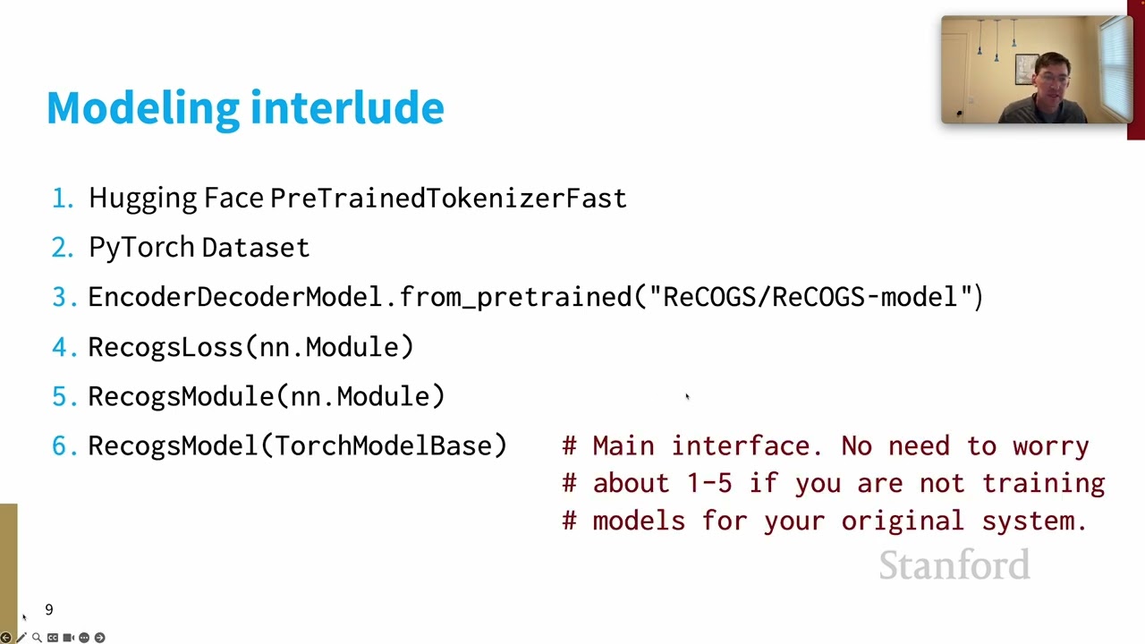
00:06:03.040 | After question one, I'll warn you there is sort of a long modeling interlude.
00:06:08.080 | I've provided all the pieces that you need to train your own Recogs models.
00:06:13.000 | You don't necessarily have to do that, but I wanted to provide them so that you could
00:06:16.760 | explore that as an avenue for your original systems.
00:06:20.940 | So let me walk you through this interlude.
00:06:22.640 | The first step is a hugging face tokenizer.
00:06:26.280 | I'll confess to you that my original plan was to have this be one of the homework questions,
00:06:30.820 | but I found writing this hugging face tokenizer to be so difficult and so confusing that I
00:06:37.400 | decided not to burden you with it.
00:06:39.360 | So I'm instead offering you this tokenizer in the hopes that you can benefit from it
00:06:43.760 | and maybe modify it for your own tasks down the line.
00:06:48.180 | The PyTorch dataset is similar.
00:06:50.160 | This is a dataset for Recogs.
00:06:53.040 | I originally thought it would be a homework question, but it has some fiddly details about
00:06:57.300 | it that may be tentative about doing that.
00:06:59.820 | So instead, I am just giving it to you.
00:07:04.340 | Step three is a pre-trained Recogs model.
00:07:07.760 | Zen trained this model.
00:07:09.220 | It is an outstanding Recogs model, and the idea is that you can just load it in and then
00:07:14.220 | make use of it.
00:07:15.660 | For your original system, you might fine tune this model or do something else to it, but
00:07:19.660 | you don't need to do that.
00:07:21.940 | For the homework question that comes next, you simply use this as a pre-trained model
00:07:26.660 | and explore its predictions.
00:07:29.820 | The next step is Recogs loss, and this is a simple PyTorch module that helps me make
00:07:35.980 | the model that Zen trained compatible with the code that we have for this course in general
00:07:40.920 | so that it's easy for you to fine tune the model if you want to.
00:07:44.860 | So that's a small detail.
00:07:47.340 | Then we have Recogs module, and this is a lightweight wrapper around Zen's model that
00:07:51.740 | is again designed to help us be compatible with the underlying optimization code in particular
00:07:57.860 | that we have in our course code base.
00:08:01.300 | And then finally, the interlude ends at step six with Recogs module.
00:08:06.500 | This Recogs model, sorry, this is the main interface and is the only one that you need
00:08:11.900 | to worry about if you're not training models for your original system.
00:08:17.000 | If you're not doing that, if you're pursuing another avenue, then you can more or less
00:08:20.420 | ignore one through five and just focus on six and treat it as a simple interface for
00:08:25.780 | loading Zen's model and using it.
00:08:28.760 | But I'm hoping that some of you want to dig deeper into how this model is trained and
00:08:33.840 | maybe improve it.
00:08:35.200 | And in that case, steps one through five will be especially useful to you.
00:08:40.020 | So that's why they're all embedded in the notebook.
00:08:43.780 | Having made it through the interlude, we now get to question two, which is exploring predictions
00:08:48.380 | of the model.
00:08:49.380 | For this question, you just use Zen's trained Recogs model out of the box.
00:08:54.600 | And what you're doing is continuing the data analysis that you began in question one.
00:09:00.500 | So you complete a function called category assess.
00:09:03.980 | And the name of the game here is to discover for yourselves that this really good model
00:09:09.120 | struggles really a lot with the proper names that are in unfamiliar positions, exactly
00:09:15.060 | the names that you identified for question one.
00:09:18.340 | So you can see the hypothesis behind Cogs and Recogs validated here.
00:09:24.860 | Novel combinations of these elements, however simple, turn out to be challenging for a really
00:09:30.060 | good model.
00:09:33.500 | Before proceeding, I wanted to say one thing about Recogs assessment.
00:09:36.820 | And again, we'll talk more in detail about this in the main screencast for the unit.
00:09:41.420 | But just quickly, the goal of Recogs is really to test for semantic interpretation and get
00:09:47.280 | past some of the incidental details of logical form.
00:09:51.020 | So our evaluation code is somewhat complicated.
00:09:54.580 | Here are three instructive examples.
00:09:56.940 | For Recogs, unlike for Cogs, the precise names of bound variables do not matter.
00:10:02.780 | So for example, these two logical forms here are called equivalent, even though the first
00:10:08.380 | logical form uses the variable four and the second logical form uses the variable seven.
00:10:13.940 | The idea is that since all these variables are implicitly bound for Recogs and Cogs,
00:10:20.100 | we don't care about their particular identity, just the binding relationships that they establish.
00:10:25.180 | And those are the same in these two cases.
00:10:28.740 | Here's another case.
00:10:29.740 | The order of conjuncts does not matter.
00:10:32.140 | That seems intuitive semantically, and we wanted it to be realized in our evaluation
00:10:37.020 | code.
00:10:38.020 | So dog and happy and happy and dog evaluate to true.
00:10:42.460 | The order of the conjuncts is incidental.
00:10:45.580 | However, consistency of variable names does matter.
00:10:49.780 | So this pair evaluates to false because the first one uses dog and happy.
00:10:57.700 | It has both a variable four for both of those predications, whereas the second one has dog
00:11:02.300 | of four and happy of seven.
00:11:04.420 | And that is semantically distinct.
00:11:06.100 | Now we're talking presumably about two distinct elements, whereas the first logical form is
00:11:10.420 | about one.
00:11:11.780 | And so we arrive at a conclusion that these are semantically not equivalent.
00:11:16.240 | So that's three kind of cases that give you a feel for what we're trying to do with this
00:11:19.780 | evaluation, which is really get at semantic equivalence, even where logical forms vary.
00:11:28.060 | Final question for the main part of the homework, question three, switches gears entirely.
00:11:33.300 | This is a basic in-context learning approach.
00:11:36.940 | And the idea here is to just get you over the hill in terms of using DSP as we did in
00:11:42.740 | homework two and applying it to this new case.
00:11:46.180 | And my thinking here is that if I push you a little bit to write your first DSP program
00:11:50.500 | for recogs, you might try more versions of that and really make progress.
00:11:55.800 | So here's the kind of logical-- here's the kind of prompt that you'll offer to the model.
00:12:00.100 | We've got a couple of demonstrations, input, and then the task for the model is to generate
00:12:04.540 | a new logical form.
00:12:06.740 | And the task here for you in terms of coding is to just write a very simple DSP program.
00:12:12.060 | It is simple indeed.
00:12:13.620 | As I said, my hope is that it's kind of inspiring you to do more sophisticated things, maybe
00:12:18.700 | for your original system.
00:12:21.380 | I will warn you that even for our best large language models, they superficially seem to
00:12:27.440 | understand what this task is about.
00:12:29.860 | And when you glance at the logical forms that they predict, they often look kind of good.
00:12:34.400 | But then you run the evaluation code and you get zero right, and you realize that kind
00:12:39.260 | of good is not really sufficient for this task.
00:12:42.400 | You need to be exactly correct.
00:12:44.900 | And these large language models seem to struggle to be exactly correct at this semantic parsing
00:12:49.860 | task.
00:12:51.660 | Finally, question four, as usual, you're doing your original system.
00:12:58.020 | For your original system, you can do anything you want.
00:13:01.580 | The only constraint is that you cannot train your system on any examples from the generalization
00:13:07.940 | splits, nor can the output representations from those examples be included in any prompts
00:13:13.740 | that you use for in-context learning.
00:13:17.020 | The idea here is that we want to preserve the sanctity of the generalization splits
00:13:21.420 | to really get a glimpse of whether or not systems are generalizing in the way that we
00:13:26.220 | care about.
00:13:28.640 | With that rule in place, I thought I would just review a few original system ideas.
00:13:32.740 | And remember, this is not meant to be exhaustive, but rather just inspiring about some potential
00:13:37.460 | avenues.
00:13:38.540 | So here they are.
00:13:39.540 | You could write a DSP program.
00:13:41.400 | You could do further training of R model.
00:13:44.280 | You could use a pre-trained model.
00:13:46.320 | You could train from scratch.
00:13:48.400 | Maybe you could even write a symbolic solver.
00:13:50.780 | And there might be other things that you can do.
00:13:53.380 | Let me elaborate just briefly on a few of these options.
00:13:56.220 | So here, if you want to further train R model, that should be very easy.
00:14:01.860 | This little snippet of code here loads in the model that Zen trained.
00:14:06.200 | And then you can see with this here, I'm doing just a little bit of additional fine tuning
00:14:11.200 | of that model on a few of the dev examples, which is fine to do because our focus is on
00:14:16.260 | those gen splits.
00:14:17.920 | And what I've done in this snippet is expose a lot of the different optimization parameters
00:14:21.780 | because I think you'd really want to think about how best to set up this model to get
00:14:26.240 | some more juice out of the available data from this further training, essentially.
00:14:33.520 | But I've also, in the notebook, offered you code that shows how easy it is to take our
00:14:38.600 | starting point and modify it to use a pre-trained model.
00:14:43.220 | Here what I've done really is just write a T5 Recogs module to load in the T5 model.
00:14:49.220 | And then T5 Recogs model is the primary interface.
00:14:52.720 | And now what you've got is a device that loads in T5.
00:14:57.240 | And it won't work at all if you try to use it directly to make predictions about the
00:15:01.160 | Recogs task.
00:15:02.160 | It will actually sort of amusingly translate your examples into German.
00:15:06.720 | But you could fine tune T5 so that it can do the Recogs task with the hypothesis that
00:15:12.240 | the pre-training that T5 underwent is useful for helping with the generalization splits
00:15:19.440 | in particular.
00:15:21.320 | And very similar code could be modified so that you train from scratch by simply loading
00:15:25.460 | in with Hugging Face code random parameters that might have the structure of a BERT model
00:15:31.480 | or something like that.
00:15:32.960 | Hugging Face makes that very easy.
00:15:35.280 | And you could explore different variants, essentially, of training from scratch on the
00:15:40.040 | Recogs task.
00:15:42.520 | And I'll leave other options for you to think about.
00:15:44.680 | I'm really keen to see what you all do with the Recogs data.
00:15:50.040 | And then finally, for the bake-off, this is straightforward.
00:15:52.920 | There's a TSV file that contains some test cases.
00:15:56.620 | Those are generalization test cases.
00:15:58.800 | You just need to add a column prediction, which contains your predicted logical forms.
00:16:03.680 | And then this final code snippet here is what you do to write that to disk for uploading
00:16:08.560 | to the Gradescope autograder.
00:16:10.840 | And we'll see how you all do on this surprisingly very challenging task of semantic interpretation.
00:16:17.520 | Thank you.
00:16:18.520 | [END]
00:16:18.520 | [BLANK_AUDIO]