Intro to Machine Learning: Lesson 3

00:00:00.000 | Last lesson, we looked at what random forests are, and we looked at some of the tweaks that

00:00:10.540 | we could use to make them work better.

00:00:17.520 | So in order to actually practice this, we needed to have a Jupyter notebook environment

00:00:23.420 | running, so we can either install Anaconda on our own computers, we can use AWS, or we

00:00:31.920 | can use cressel.com that has everything up and running straight away, or else paperspace.com

00:00:37.920 | also works really well.

00:00:40.320 | So assuming that you've got all that going, hopefully you've had a chance to practice

00:00:44.800 | running some random forests this week.

00:00:47.080 | I think one of the things to point out though is that before we did any tweaks of any hyperparameters

00:00:53.840 | or any tuning at all, the raw defaults already gave us a very good answer for an actual dataset

00:01:01.240 | that we've got on Kaggle.

00:01:02.440 | So the tweaks aren't always the main piece, they're just tweaks.

00:01:08.900 | Sometimes they're totally necessary, but quite often you can go a long way without doing

00:01:15.360 | any treats at all.

00:01:18.280 | So today we're going to look at something I think maybe even more important than building

00:01:25.320 | a predictive model that's good at predicting, which is to learn how to interpret that model

00:01:30.640 | to find out what it says about your data, to actually understand your data better by

00:01:37.200 | using machine learning.

00:01:47.200 | Things like random forests are black boxes that hide meaning from us.

00:01:52.080 | You'll see today that the truth is quite the opposite.

00:01:55.040 | The truth is that random forests allow us to understand our data deeper and more quickly

00:02:02.080 | than traditional approaches.

00:02:04.840 | The other thing we're going to learn today is how to look at larger datasets than those

00:02:11.640 | which you can import with just the defaults.

00:02:15.840 | And specifically we're going to look at a dataset with over 100 million rows, which

00:02:19.760 | is the current Kaggle competition for groceries for past year.

00:02:25.080 | Did anybody have any questions outside of those two areas since we're covering that

00:02:29.400 | today or comments that they want to talk about?

00:02:42.440 | Can you just talk a little bit about in general, I understand the details more now of random

00:02:47.320 | forests, but when do you know this is an applicable model to use?

00:02:51.680 | In general, I should try random forests here because that's the part that I'm still like,

00:02:56.120 | if I'm told to I can.

00:02:58.120 | So the short answer is, I can't really think of anything offhand that it's definitely not

00:03:07.440 | going to be at least somewhat useful for, so it's always worth trying.

00:03:13.480 | I think really the question is, in what situations should I try other things as well?

00:03:20.800 | And the short answer to that question is for unstructured data, what I call unstructured

00:03:24.800 | data. So where all the different data points represent the same kind of thing, like a waveform

00:03:30.640 | in a sound or speech, or the words in a piece of text, or the pixels in an image, you're

00:03:36.360 | almost certainly going to want to try deep learning.

00:03:42.720 | And then outside of those two, there's a particular type of model we're going to look at today

00:03:50.080 | called a collaborative filtering model, which so happens that the groceries competition

00:03:56.280 | is of that kind, where neither of those approaches are quite what you want without some tweaks

00:04:02.120 | to them.

00:04:03.120 | So that would be the other main one.

00:04:05.240 | If anybody thinks of other places where maybe neither of those techniques is the right thing

00:04:20.960 | to use, mention it on the forums, even if you're not sure, so we can talk about it because

00:04:26.600 | I think this is one of the more interesting questions.

00:04:32.040 | And to some extent it is a case of practice and experience, but I do think there are two

00:04:39.000 | main classes to know about.

00:04:47.120 | Last week, at the point where we had done some of the key steps, like the CSV reading

00:04:59.720 | in particular, which took a minute or two, at the end of that we saved it to a feather

00:05:04.560 | format file.

00:05:05.560 | And just to remind you, that's because this is basically almost the same format that it

00:05:10.800 | lives in in RAM, so it's ridiculously fast to read and write stuff from feather format.

00:05:16.840 | So what we're going to do today is we're going to look at lesson 2, RF interpretation, and

00:05:23.440 | the first thing we're going to do is read that feather format file.

00:05:29.200 | Now one thing to mention is a couple of you pointed out during the week, a really interesting

00:05:36.840 | little bug or little issue, which is in the proc df function.

00:05:45.280 | The proc df function, remember, finds the numeric columns which have missing values

00:05:52.160 | and creates an additional boolean column, as well as replacing the missing with medians,

00:06:00.080 | and also turns the categorical objects into the integer codes, the main things it does.

00:06:09.840 | And a couple of you pointed out some key points about the missing value handling.

00:06:14.960 | The first one is that your test set may have missing values in some columns that weren't

00:06:23.240 | in your training set or vice-versa.

00:06:26.800 | And if that happens, you're going to get an error when you try to do the random forest,

00:06:30.160 | because it's going to say if that is missing field appeared in your training set but not

00:06:35.960 | in your test set that ended up in the model, it's going to say you can't use that data

00:06:42.400 | set with this model because you're missing one of the columns it requires.

00:06:47.280 | That's problem number 1.

00:06:49.140 | Problem number 2 is that the median of the numeric values in the test set may be different

00:06:57.760 | for the training set, so it may actually process it into something which has different semantics.

00:07:06.720 | So I thought that was a really interesting point.

00:07:09.160 | So what I did was I changed prop df, so it returns a third thing, nas.

00:07:17.640 | And the nas thing it returns, it doesn't matter in detail what it is, but I'll tell you just

00:07:23.160 | so you know, that's a dictionary where the keys are the names of the columns that have

00:07:29.400 | missing values, and the values of the dictionary are the medians.

00:07:34.600 | And so then optionally you can pass nas as an additional argument to prop df, and it'll

00:07:43.640 | make sure that it adds those specific columns and it uses those specific medians.

00:07:50.040 | So it's giving you the ability to say process this test set in exactly the same way as we

00:07:57.120 | process this training set.

00:08:07.160 | So I just did that like yesterday or the day before.

00:08:10.760 | In fact that's a good point.

00:08:12.320 | Before you start doing work any day, I would start doing a git pull, and if something's

00:08:19.520 | not working today that was working yesterday, check the forum where there will be an explanation

00:08:24.000 | of why.

00:08:27.840 | This library in particular is moving fast, but pretty much all the libraries that we

00:08:31.640 | use, including PyTorch in particular, move fast.

00:08:34.780 | And so one of the things to do if you're watching this through the MOOC is to make sure that

00:08:40.320 | you've got a course.fast.ai and check the links there because there will be links saying

00:08:45.560 | oh these are the differences from the course, and so they're kept up to date so that you're

00:08:50.520 | never going to -- because I can't edit what I'm saying, I can only edit that.

00:08:56.000 | But do a git pull before you start each day.

00:09:03.280 | So I haven't actually updated all of the notebooks to add the extra return value.

00:09:10.360 | I will over the next couple of days, but if you're using them you'll just need to put

00:09:13.520 | an extra comma, otherwise you'll get an error that it's returned 3 things and you only have

00:09:19.200 | room for 2 things.

00:09:26.200 | What I want to do before I talk about interpretation is to show you what the exact same process

00:09:33.640 | looks like when you're working with a really large dataset.

00:09:38.920 | And you'll see it's kind of almost the same thing, but there's going to be a few cases

00:09:46.440 | where we can't use the defaults, because the defaults just run a little bit too slowly.

00:09:53.780 | So specifically I'm going to look at the Cabo Groceries competition, specifically -- what's

00:10:06.560 | it called?

00:10:07.560 | Here it is.

00:10:08.560 | Compress your favorite grocery sales forecasting.

00:10:12.280 | So this competition -- who is entering this competition?

00:10:20.000 | Okay, a lot of people.

00:10:22.740 | Who would like to have a go at explaining what this competition involves, what the data

00:10:29.360 | is and what you're trying to predict?

00:10:34.760 | >> Okay, trying to predict the items on the shelf depending on lots of factors, like oil

00:10:40.960 | prices.

00:10:41.960 | So when you're predicting the items on the shelf, what are you actually predicting?

00:10:46.760 | >> How much do you need to have in stock to maximize their --

00:10:50.520 | >> It's not quite what we're predicting, but we'll try and fix that at the moment.

00:10:54.620 | >> And then there's a bunch of different datasets that you can use to do that.

00:10:57.360 | There's oil prices, there's stores, there's locations, and each of those can be used to

00:11:03.080 | try to predict it.

00:11:04.080 | Does anybody want to have a go at expanding on that?

00:11:12.680 | >> All right.

00:11:14.680 | So we have a bunch of information on different products.

00:11:19.160 | So we have --

00:11:20.160 | >> Let's just fill up a little bit higher.

00:11:23.080 | >> All right.

00:11:24.080 | So for every store, for every item, for every day, we have a lot of related information

00:11:30.760 | available, like the location where the store was located, the class of the product, and

00:11:39.920 | the units sold.

00:11:41.760 | And then based on this, we are supposed to forecast in a much shorter time frame compared

00:11:46.720 | to the training data.

00:11:48.200 | For every item number, how much we think it's going to sell, so only the units and nothing

00:11:53.040 | else.

00:11:54.040 | >> Okay, good.

00:11:55.040 | Somebody can help get that back here.

00:12:02.920 | So your ability to explain the problem you're working on is really, really important.

00:12:10.580 | So if you don't currently feel confident of your ability to do that, practice with someone

00:12:16.640 | who is not in this competition.

00:12:18.960 | Tell them all about it.

00:12:21.400 | So in this case, or in any case really, the key things to understand a machine learning

00:12:28.160 | problem would be to say what are the independent variables and what is the dependent variable.

00:12:32.360 | So the dependent variable is the thing that you're trying to predict.

00:12:35.800 | The thing you're trying to predict is how many units of each kind of product were sold

00:12:43.040 | in each store on each day during a two-week period.

00:12:48.080 | So that's the thing that you're trying to predict.

00:12:50.520 | The information you have to predict is how many units of each product at each store on

00:12:57.920 | each day were sold in the last few years, and for each store some metadata about it,

00:13:06.400 | like where is it located and what class of store is it.

00:13:09.840 | For each type of product, you have some metadata about it, such as what category of product

00:13:15.640 | is it and so forth.

00:13:17.600 | For each date, we have some metadata about it, such as what was the oil price on that

00:13:23.240 | date.

00:13:24.520 | So this is what we would call a relational dataset.

00:13:27.000 | A relational dataset is one where we have a number of different pieces of information

00:13:32.360 | that we can join together.

00:13:35.800 | Specifically this kind of relational dataset is what we would refer to as a star schema.

00:13:41.920 | A star schema is a kind of data warehousing schema where we say there's some central transactions

00:13:48.960 | table.

00:13:49.960 | In this case, the central transactions table is train.csv, and it contains the number of

00:14:01.680 | units that were sold by date, by store ID, by item ID.

00:14:09.720 | So that's the central transactions table, very small, very simple, and then from that

00:14:13.440 | we can join various bits of metadata.

00:14:16.080 | It's called a star schema because you can imagine the transactions table in the middle

00:14:21.720 | and then all these different metadata tables join onto it, giving you more information

00:14:27.640 | about the date, the item ID and the store ID.

00:14:34.360 | Sometimes you'll also see a snowflake schema, which means there might then be additional

00:14:38.920 | information joined onto maybe the items table that tells you about different item categories

00:14:46.560 | and joined to the store table, telling you about the state that the store is in and so

00:14:50.840 | forth so you can have a whole snowflake.

00:14:55.840 | So that's the basic information about this problem, the independent variables, the dependent

00:15:05.640 | variable, and you probably also want to tell you about things like the timeframe.

00:15:13.440 | Now we start in exactly the same way as we did before, loading in exactly the same stuff,

00:15:19.280 | setting the path.

00:15:20.280 | But when we go read CSV, if you say limit memory equals false, then you're basically

00:15:29.400 | saying use as much memory as you like to figure out what kinds of data is here.

00:15:34.160 | It's going to run out of memory pretty much regardless of how much memory you have.

00:15:39.840 | So what we do in order to limit the amount of space that it takes up when we read it

00:15:45.400 | in is we create a dictionary for each column name to the data type of that column.

00:15:52.440 | And so for you to create this, it's basically up to you to run less or head or whatever

00:15:58.520 | on the data set to see what the types are and to figure that out and pass them in.

00:16:04.600 | So then you can just pass in data type equals with that dictionary.

00:16:10.080 | And so check this out, we can read in the whole CSV file in 1 minute and 48 seconds,

00:16:21.720 | and there are 125.5 million rows.

00:16:30.280 | So when people say Python's slow, no Python's not slow.

00:16:37.240 | Python can be slow if you don't use it right, but we can actually pass 125 million CSV records

00:16:44.680 | in less than 2 minutes.

00:16:49.400 | I'm going to put my language hat on for just a moment.

00:16:54.200 | Actually if it's fast, almost certainly it's going to see.

00:16:58.760 | So Python is a wrapper around a bunch of C code usually.

00:17:04.200 | So if Python itself isn't actually very fast.

00:17:12.240 | So that was Terrence Parr who writes things for writing programming languages for a living.

00:17:20.920 | Python itself is not fast, but almost everything we want to do in Python and data science has

00:17:26.720 | been written for us in C, or actually more often in Python, which is a Python-like language

00:17:32.360 | which compiles to C. So most of the stuff we run in Python is actually running not just

00:17:38.600 | C code, but actually in Pandas a lot of it's written in assembly language, it's heavily

00:17:42.880 | optimized, behind the scenes a lot of that is going back to actually calling Fortran-based

00:17:48.880 | libraries for a linear algebra.

00:17:51.440 | So there's layers upon layer of speed that actually allow us to spend less than 2 minutes

00:17:57.320 | reading in that much data.

00:18:00.440 | If we wrote our own CSV reader in pure Python, it would take thousands of times, at least

00:18:08.400 | thousands of times longer than the optimized versions.

00:18:13.640 | So for us, what we care about is the speed we can get in practice.

00:18:18.160 | So this is pretty cool.

00:18:20.160 | As well as telling it what the different data types were, we also have to tell it as before

00:18:25.600 | which things you want to parse as dates.

00:18:33.280 | I've noticed that in this dictionary, you specify in 64, 33, and 8.

00:18:39.280 | I was wondering in practice, is it faster if you all specify them to be slower, or any

00:18:47.620 | performance consideration?

00:18:49.280 | So the key performance consideration here was to use the smallest number of bits that

00:18:54.400 | I could to fully represent the column.

00:18:57.120 | So if I had used n8 for item number, there are more than 255 item numbers.

00:19:02.360 | More specifically, the maximum item number is bigger than 255.

00:19:06.120 | So on the other hand, if I had used n64 for store number, it's using more bits than necessary.

00:19:13.640 | Given that the whole purpose here was to avoid running out of RAM, we don't want to be using

00:19:18.160 | up 8 times more memory than necessary.

00:19:21.880 | So the key thing was really about memory.

00:19:24.320 | In fact when you're working with large data sets, very often you'll find the slow piece

00:19:29.760 | is the actually reading and writing to RAM, not the actual CPU operations.

00:19:35.520 | So very often that's the key performance consideration.

00:19:39.540 | Also however, as a rule of thumb, smaller data types often will run faster, particularly

00:19:47.720 | if you can use 70, so that's single instruction multiple data vectorized code.

00:19:52.720 | It can pack more numbers into a single vector to run at once.

00:20:04.840 | That was all heavily simplified and not exactly right, but right and bound for this purpose.

00:20:11.960 | Once you do this, the shuffle thing beforehand is not needed anymore, you may just send a

00:20:19.120 | random sub solution.

00:20:23.120 | Although here I've read in the whole thing, when I start, I never start by reading in

00:20:30.720 | the whole thing.

00:20:32.760 | So if you search the forum for 'shuff', you'll find some tips about how to use this UNIX

00:20:42.860 | command to get a random sample of data at the command prompt.

00:20:48.160 | And then you can just read that.

00:20:49.480 | The nice thing is that that's a good way to find out what data types to use, to read in

00:20:56.040 | a random sample and let pandas figure it out for you.

00:21:06.600 | In general, I do as much work as possible on a sample until I feel confident that I understand

00:21:13.280 | the sample before I move on.

00:21:17.440 | Having said that, what we're about to learn is some techniques for running models on this

00:21:20.980 | full dataset that are actually going to work on arbitrarily large datasets, that also I

00:21:25.120 | specifically wanted to talk about how to read in large datasets.

00:21:29.600 | One thing to mention, onPromotion objects are like saying create a general purpose Python

00:21:36.200 | data type which is slow and memory heavy.

00:21:39.560 | The reason for that is that this is a Boolean which also has missing values, and so we need

00:21:44.800 | to deal with this before we can turn it into a Boolean.

00:21:47.720 | So you can see after that, I then go ahead and let's say fill in the missing values with

00:21:51.600 | false.

00:21:52.600 | Now you wouldn't just do this without doing some checking ahead of time, but some exploratory

00:21:57.480 | data analysis shows that this is probably an appropriate thing to do, it seems that

00:22:02.000 | missing does mean false.

00:22:06.680 | Objects generally read in a string, so replace the strings true and false with actual Booleans,

00:22:11.880 | and then finally convert it to an actual Boolean type.

00:22:15.200 | So at this point, when I save this, this file now of 123 million records takes up something

00:22:23.440 | under 2.5 GB of memory.

00:22:26.160 | So you can look at pretty large datasets even on pretty small computers, which is interesting.

00:22:33.680 | So at that point, now that it's in a nice fast format, look how fast it is.

00:22:37.400 | I can save it to feather format in under 5 seconds.

00:22:41.560 | So that's nice.

00:22:43.880 | And then because pandas is generally pretty fast, you can do stuff like summarize every

00:22:50.240 | column of all 125 million records in 20 seconds.

00:22:57.760 | The first thing I looked at here is the dates.

00:23:01.200 | Generally speaking, dates are just going to be really important on a lot of the stuff

00:23:04.040 | you do, particularly because any model that you put in in practice, you're going to be

00:23:10.280 | putting it in at some date that is later than the date that you trained it by definition.

00:23:16.120 | And so if anything in the world changes, you need to know how your predictive accuracy

00:23:20.640 | changes as well.

00:23:22.120 | And so what you'll see on Kaggle and what you should always do in your on projects is

00:23:25.720 | make sure that your dates don't overlap.

00:23:27.760 | So in this case, the dates that we have in the training set go from 2013 to mid-August

00:23:34.840 | 2017, there's our first and last.

00:23:40.360 | And then in our test set, they go from 1 day later, August 16th until the end of the month.

00:23:48.720 | So this is a key thing that you can't really do any useful machine learning until you understand

00:23:55.160 | this basic piece here, which is you've got 4 years of data and you're trying to predict

00:24:03.720 | the next 2 weeks.

00:24:06.480 | So that's just a fundamental thing that you're going to need to understand before you can

00:24:10.240 | really do a good job of this.

00:24:11.920 | And so as soon as I see that, what does that say to you?

00:24:16.480 | If you wanted to now use a smaller data set, should you use a random sample, or is there

00:24:22.160 | something better you could do?

00:24:24.120 | Probably from the bottom, more recent?

00:24:34.720 | So it's like, okay, I'm going to go to a shop next week and I've got a $5 bet with my brother

00:24:44.640 | as to whether I can guess how many cans of Coke are going to be on the shelf.

00:24:48.960 | Alright, well probably the best way to do that would be to go to the shop same day of

00:24:55.640 | the previous week and see how many cans of Coke are on the shelf and guess it's going

00:24:59.280 | to be the same.

00:25:00.280 | You wouldn't go and look at how many were there 4 years ago.

00:25:07.100 | But couldn't 4 years ago that same time frame of the year be important?

00:25:11.800 | For example, how much Coke they have on the shelf at Christmas time is going to be way

00:25:14.840 | more than?

00:25:15.840 | Exactly, so there's no useful information from 4 years ago, so we don't want to entirely

00:25:23.960 | throw it away.

00:25:24.960 | But as a first step, what's the simplest possible thing?

00:25:29.680 | It's kind of like submitting the means.

00:25:31.640 | I wouldn't submit the mean of 2012 sales, I would probably submit the mean of last month's

00:25:39.160 | sales, for example.

00:25:42.560 | So yeah, we're just trying to think about how we might want to create some initial easy

00:25:48.240 | models and later on we might want to wait it.

00:25:51.760 | So for example, we might want to wait more recent dates more highly, they're probably

00:25:55.400 | more relevant.

00:25:56.400 | But we should do a whole bunch of exploratory data analysis to check that.

00:26:01.400 | So here's what the bottom of that data set looks like.

00:26:06.040 | And you can see literally it's got a date, a store number, an item number, an unit sales,

00:26:12.640 | and tells you whether or not that particular item was on sale at that particular store

00:26:18.200 | on that particular date, and then there's some arbitrary ID.

00:26:23.000 | So that's it.

00:26:26.540 | So now that we have read that in, we can do stuff like, this is interesting, again we

00:26:33.600 | have to take the log of the sales.

00:26:37.040 | And it's the same reason as we looked at last week, because we're trying to predict something

00:26:40.920 | that varies according to ratios.

00:26:43.820 | They told us in this competition that the root mean squared log error is the thing they

00:26:48.840 | care about, so we take the log.

00:26:51.680 | They mentioned also if you check the competition details, which you always should read carefully

00:26:56.920 | the definition of any project you do, they say that there are some negative sales that

00:27:01.720 | represent returns, and they tell us that we should consider them to be 0 for the purpose

00:27:07.440 | of this competition.

00:27:08.680 | So I clip the sales so that they fall between 0 and no particular maximum, so clip just

00:27:17.960 | means cut it off at that point, truncate it, and then take the log of that +1.

00:27:24.420 | Why do I do +1?

00:27:25.840 | Because again, if you check the details of the capital competition, that's what they

00:27:28.840 | tell you they're going to use is they're not actually just taking the root mean squared

00:27:32.080 | log error, but the root mean squared log +1 error, because log of 0 doesn't make sense.

00:27:41.520 | We can add the date part as usual, and again it's taking a couple of minutes.

00:27:47.160 | So I would run through all this on a sample first, so everything takes 10 seconds to make

00:27:51.640 | sure it works, just to check everything looks reasonable before I go back because I don't

00:27:55.320 | want to wait 2 minutes or something, I don't know if it's going to work.

00:27:59.720 | But as you can see, all these lines of code are identical to what we saw for the bulldozers

00:28:04.240 | competition.

00:28:07.080 | In this case, all I'm reading in is a training set.

00:28:09.400 | I didn't need to run train cats because all of my data types are already numeric.

00:28:14.840 | If they weren't, I would need to call train cats and then I would need to call apply cats

00:28:21.640 | to the same categorical codes that I now have in the training set to the validation set.

00:28:29.560 | I call prop df as before to check for missing values and so forth.

00:28:37.720 | So all of those lines of code are identical.

00:28:40.560 | These lines of code again are identical because root mean squared error is what we care about.

00:28:48.520 | And then I've got two changes.

00:28:50.040 | The first is sent RF samples, which we learned about last week.

00:28:55.080 | So we've got 120 something million records.

00:28:59.600 | We probably don't want to create a tree from 120 million something records.

00:29:04.000 | I don't even know how long that's going to take, I haven't had the time and patience

00:29:08.200 | to wait and see.

00:29:10.880 | So you could start with 10,000 or 100,000, maybe it runs in a few seconds, make sure

00:29:17.440 | it works and you can figure out how much you can run.

00:29:20.480 | And so I found getting it to a million, it runs in under a minute.

00:29:26.600 | And so the point here is there's no relationship between the size of the dataset and how long

00:29:31.880 | it takes to build the random forest.

00:29:33.840 | The relationship is between the number of estimators multiplied by the sample size.

00:29:39.720 | So the number of jobs is the number of cores that it's going to use.

00:29:53.040 | And I was running this on a computer that has about 60 cores, and I just found if you

00:29:58.200 | try to use all of them, it spends so much time spinning up jobs so it's a bit slower.

00:30:01.840 | So if you've got lots and lots of cores on your computer, sometimes you want less than

00:30:07.560 | negative 1 means use every single core.

00:30:10.680 | There's one more change I made which is that I converted the data frame into an array of

00:30:18.040 | floats and then I fitted on that.

00:30:21.640 | Why did I do that?

00:30:24.160 | Because internally inside the random forest code, they do that anyway.

00:30:29.560 | And so given that I wanted to run a few different random forests with a few different hyperparameters,

00:30:34.640 | by doing it once myself, I saved that minute 37 seconds.

00:30:41.040 | So if you run a line of code and it takes quite a long time, so the first time I ran

00:30:49.660 | this random forest progressor, it took 2 or 3 minutes, and I thought I don't really want

00:30:53.600 | to wait 2 or 3 minutes, you can always add in front of the line of code prun, percent

00:31:01.760 | prun.

00:31:02.760 | So what percent prun does is it runs something called a profiler.

00:31:07.240 | And what a profiler does is it will tell you which lines of code behind the scenes took

00:31:12.200 | the most time.

00:31:13.200 | And in this case I noticed that there was a line of code inside scikit-learn that was

00:31:18.780 | this line of code, and it was taking all the time, nearly all the time.

00:31:22.560 | And so I thought I'll do that first and then I'll pass in the result and it won't have

00:31:26.120 | to do it again.

00:31:27.600 | So this thing of looking to see which things is taking up the time is called profiling.

00:31:33.560 | And in software engineering, it's one of the most important tools you have.

00:31:37.520 | Data scientists really underappreciate this tool, but you'll find amongst conversations

00:31:44.160 | on GitHub issues or on Twitter or whatever amongst the top data scientists, they're sharing

00:31:49.240 | and talking about profiles all the time.

00:31:51.640 | And that's how easy it is to get a profile.

00:31:54.760 | So for fun, try running prun from time to time on stuff that's taking 10-20 seconds and

00:32:02.840 | see if you can learn to interpret and use profiler outputs.

00:32:07.320 | Even though in this case I didn't write this scikit-learn, plus I was still able to use

00:32:14.040 | the profiler to figure out how to make it run over twice as fast by avoiding recalculating

00:32:21.080 | this each time.

00:32:22.980 | So in this case, I built my regressor, I decided to use 20 estimators.

00:32:27.800 | Something else that I noticed in the profiler is that I can't use OOB score when I use set-RF

00:32:33.320 | samples.

00:32:34.320 | Because if I do, it's going to use the other 124 million rows to calculate the OOB score,

00:32:41.960 | which is still going to take forever.

00:32:45.440 | So I may as well have a proper validation set anyway, besides which I want a validation

00:32:49.640 | set that's the most recent dates rather than it's random.

00:32:53.720 | So if you use set-RF samples on a large data set, don't put the OOB score parameter in

00:33:01.120 | because it takes forever.

00:33:04.320 | So that got me a 0.76 validation root mean squared log error, and then I tried fiddling

00:33:12.760 | around with different min-samples.

00:33:14.320 | So if I decrease the min-samples from 100 to 10, it took a little bit more time to run

00:33:19.620 | as we would expect.

00:33:22.360 | And the error went down from 76 to 71, so that looked pretty good.

00:33:28.680 | So I kept decreasing it down to 3, and that brought this error down to 0.70.

00:33:33.560 | When I decreased it down to 1, it didn't really help.

00:33:36.800 | So I kind of had a reasonable random forest.

00:33:41.440 | When I say reasonable, though, it's not reasonable in the sense that it does not give a good

00:33:50.600 | result on the later morning.

00:33:53.640 | And so this is a very interesting question about why is that.

00:33:57.600 | And the reason is really coming back to Savannah's question earlier, where might random forests

00:34:03.420 | not work as well.

00:34:05.320 | Let's go back and look at the data.

00:34:08.440 | Here's the entire dataset, here's all the columns we used.

00:34:12.840 | So the columns that we have to predict with are the date, the store number, the item number,

00:34:20.800 | and whether it was on promotion or not.

00:34:23.880 | And then of course we used add date part, so there's also going to be day of week, day

00:34:28.080 | of month, day of year, is quarter, start, etcetera, etcetera.

00:34:33.440 | So if you think about it, most of the insight around how much of something do you expect

00:34:43.000 | to sell tomorrow is likely to be very wrapped up in the details about where is that store,

00:34:50.040 | what kind of things do they tend to sell at that store, for that item, what category of

00:34:54.560 | item is it, if it's like fresh bread, they might not sell much of it on Sundays because

00:35:02.600 | on Sundays, fresh bread doesn't get made, where else it's gasoline, maybe they're going

00:35:08.400 | to sell a lot of gasoline because on Sundays people go and fill up their cart with a wick

00:35:13.280 | ahead.

00:35:14.280 | Now a random forest has no ability to do anything other than create a bunch of binary splits

00:35:20.380 | on things like day of week, store number, item number.

00:35:23.360 | It doesn't know which one represents gasoline.

00:35:27.120 | It doesn't know which stores are in the center of the city versus which ones are out in the

00:35:32.120 | streets.

00:35:33.120 | It doesn't know any of these things.

00:35:37.060 | Its ability to really understand what's going on is somewhat limited.

00:35:42.200 | So we're probably going to need to use the entire four years of data to even get some

00:35:46.880 | useful insights.

00:35:48.480 | But then as soon as we start using the whole four years of data, a lot of the data we're

00:35:52.160 | using is really old.

00:35:55.600 | So interestingly, there's a Kaggle kernel that points out that what you could do is

00:36:02.560 | just take the last two weeks and take the average sales by date, by store number, by

00:36:11.920 | item number and just submit that.

00:36:15.440 | If you just submit that, you come about 30th.

00:36:21.800 | So for those of you in the groceries, Terrence has a comment or a question.

00:36:31.160 | I think this may have tripped me up actually.

00:36:32.760 | I think you said date, store, item.

00:36:34.840 | I think it's actually store, item, sales and then you mean across date.

00:36:38.200 | Oh yeah, you're right.

00:36:39.200 | It's store, item and on promotion.

00:36:42.240 | On promotion, yes.

00:36:46.560 | If you do it by date as well, you end up.

00:36:50.320 | So each row represents basically a cross tabulation of all of the sales in that store for that

00:36:56.920 | item.

00:36:57.920 | So if you put date in there as well, there's only going to be one or two items being averaged

00:37:03.560 | in each of those cells, which is too much variation, basically, it's too sparse.

00:37:08.360 | It doesn't give you a terrible result, but it's not 30th.

00:37:17.560 | So your job if you're looking at this competition, and we'll talk about this in the next class,

00:37:23.400 | is how do you start with that model and make it a little bit better.

00:37:31.960 | Because if you can, then by the time we meet up next, hopefully you'll be above the top

00:37:38.600 | 30.

00:37:39.640 | Because Kaggle being Kaggle, lots of people have now taken this kernel and submitted it,

00:37:44.200 | and they all have about the same score, and the scores are ordered not just by score but

00:37:48.800 | by date submitted.

00:37:50.280 | So if you now submit this kernel, you're not going to be 30th because you're way down the

00:37:54.600 | list of when it was submitted.

00:37:56.920 | But if you can do a tiny bit better, you're going to be better than all of those people.

00:38:01.880 | So how can you make this a tiny bit better?

00:38:10.960 | Would you try to capture seasonality and trend effects by creating new columns?

00:38:15.320 | These are the average sales in the month of August, these are the average sales for this

00:38:18.560 | year?

00:38:19.560 | Yeah, I think that's a great idea.

00:38:20.800 | So the thing for you to think about is how to do that.

00:38:26.480 | And so see if you can make it work.

00:38:29.440 | Because there are details to get right, which I know Terrence has been working on this for

00:38:33.320 | the last week, and he's almost crazy.

00:38:38.440 | The details are difficult, they're not intellectually difficult, they're kind of difficult in the

00:38:46.920 | way that makes you want to head back to your desk at 2am.

00:38:50.960 | And this is something to mention in general.

00:38:55.280 | The coding you do for machine learning is incredibly frustrating and incredibly difficult.

00:39:05.320 | If you get a detail wrong, much of the time it's not going to give you an exception, it

00:39:14.840 | will just silently be slightly less good than it otherwise would have been.

00:39:19.140 | And if you're on Kaggle, at least you know, okay well I'm not doing as well as other people

00:39:23.400 | on Kaggle.

00:39:24.400 | But if you're not on Kaggle, you just don't know.

00:39:27.520 | You don't know if your company's model is like half as good as it could be because you

00:39:31.840 | made a little mistake.

00:39:33.680 | So that's one of the reasons why practicing on Kaggle now is great, because you're going

00:39:38.960 | to get practice in finding all of the ways in which you can infuriatingly screw things

00:39:44.800 | up.

00:39:45.800 | And you'll be amazed, like for me there's an extraordinary array of them.

00:39:50.000 | But as you get to know what they are, you'll start to know how to check for them as you

00:39:54.880 | go.

00:39:55.880 | And so the only way, you should assume every button you press, you're going to press the

00:40:01.160 | wrong button.

00:40:02.560 | And that's fine as long as you have a way to find out.

00:40:07.000 | We'll talk about that more during the course, but unfortunately there isn't a set of specific

00:40:16.600 | things I can tell you to always do.

00:40:18.640 | You just always have to think like, okay, what do I know about the results of this thing

00:40:24.280 | I'm about to do?

00:40:25.280 | I'll give you a really simple example.

00:40:29.400 | If you've actually created that basic entry where you take the mean by date, by store

00:40:34.800 | number, by on promotion, and you've submitted it and you've got a reasonable score, and

00:40:40.040 | then you think you've got something that's a little bit better, and you do predictions

00:40:44.360 | for that, how about you now create a scatterplot showing the predictions of your average model

00:40:52.160 | on one axis versus the predictions of your new model on the other axis?

00:40:56.160 | You should see that they just about form a line.

00:41:00.960 | And if they don't, then that's a very strong suggestion that you screwed something up.

00:41:06.320 | So that would be an example.

00:41:08.280 | Can you pass that one to the end of that row, possible two steps?

00:41:17.440 | So for a problem like this, unlike the car insurance problem on Taggle where columns

00:41:24.960 | are unnamed, we know what the columns represent and what they are.

00:41:31.760 | How often do you pull in data from other sources to supplement that?

00:41:39.280 | Maybe like weather data, for example, or how often is that used?

00:41:44.840 | Very often.

00:41:45.840 | And so the whole point of this star schema is that you've got your central table and

00:41:51.920 | you've got these other tables coming off that provide metadata about it.

00:41:55.920 | So for example, weather is metadata about a date.

00:42:01.520 | On Kaggle specifically, most competitions have the rule that you can use external data

00:42:08.720 | as long as you post on the forum that you're using it and that it's publicly available.

00:42:16.400 | But you have to check on a competition by competition basis, they will tell you.

00:42:20.720 | So with Kaggle, you should always be looking for what external data could I possibly leverage

00:42:27.280 | here.

00:42:28.280 | So are we still talking about how to tweak this data set?

00:42:39.760 | If you wish.

00:42:40.920 | Well, I'm not familiar with the countries here, so maybe.

00:42:45.400 | This is Ecuador.

00:42:46.400 | Ecuador.

00:42:47.400 | So maybe I would start looking for Ecuador's holidays and shopping holidays, maybe when

00:42:58.160 | they have a three-day weekend or a week off.

00:43:00.480 | Actually that information is provided in this case.

00:43:04.360 | And so in general, one way of tackling this kind of problem is to create lots and lots

00:43:12.360 | of new columns containing things like average number of sales on holidays, average percent

00:43:19.160 | change in sale between January and February, and so on and so forth.

00:43:23.560 | And so if you have a look at, there's been a previous competition on Kaggle called Rossman

00:43:31.280 | Store Sales that was almost identical.

00:43:34.280 | It was in Germany in this case for a major grocery chain.

00:43:38.880 | How many items are sold by day, by item type, by store.

00:43:43.400 | In this case, the person who won, quite unusually actually, was something of a domain expert

00:43:50.520 | in this space.

00:43:51.520 | They're actually a specialist in doing logistics predictions.

00:43:56.320 | And this is basically what they did, he's a professional sales forecast consultant.

00:44:04.360 | He created just lots and lots and lots of columns based on his experience of what kinds

00:44:09.280 | of things tend to be useful for making predictions.

00:44:13.360 | That's an approach that can work.

00:44:17.160 | The third place team did almost no feature engineering, however, and also they had one

00:44:23.160 | big oversight, which I think they would have won if they hadn't had it.

00:44:26.520 | So you don't necessarily have to use this approach.

00:44:30.560 | So anyway, we'll be learning a lot more about how to win this competition, and ones like

00:44:37.360 | it as we go.

00:44:40.120 | They did interview the third place team, so if you google for Kaggle or Rossman, you'll

00:44:44.600 | see it.

00:44:45.600 | The short answer is they used big money.

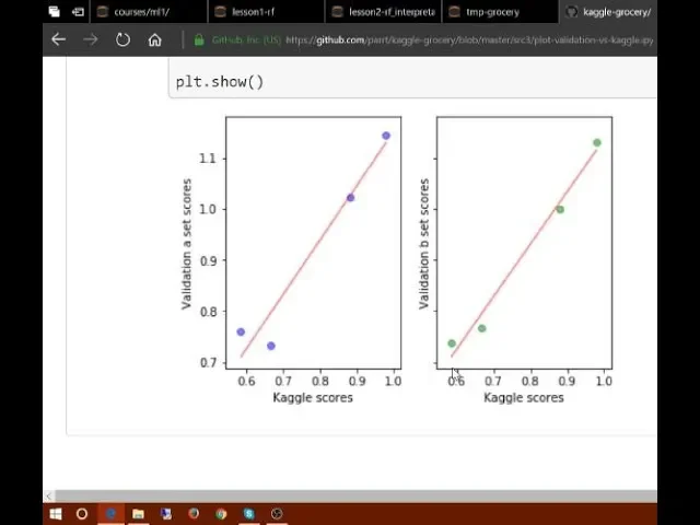
00:44:50.120 | So one of the things, and these are a couple of charts, Terrence is actually my teammate

00:44:54.360 | on this competition, so Terrence drew a couple of these charts for us, and I want to talk

00:44:59.080 | about this.

00:45:01.400 | If you don't have a good validation set, it's hard if not impossible to create a good model.

00:45:09.120 | So in other words, if you're trying to predict next month's sales and you try to build a

00:45:18.040 | model and you have no way of really knowing whether the models you built are good at predicting

00:45:23.640 | sales a month ahead of time, then you have no way of knowing when you put your model

00:45:27.840 | in production whether it's actually going to be any good.

00:45:33.000 | So you need a validation set that you know is reliable at telling you whether or not

00:45:39.360 | your model is likely to work well when you put it into production or use it on the test

00:45:45.600 | set.

00:45:47.380 | So in this case, what Terrence has plotted here is, so normally you should not use your

00:45:54.080 | test set for anything other than using it right at the end of the competition to find

00:46:00.840 | out how you've got.

00:46:01.840 | But there's one thing I'm going to let you use the test set for in addition, and that

00:46:06.680 | is to calibrate your validation set.

00:46:09.320 | So what Terrence did here was he built four different models, some which he thought would

00:46:14.620 | be better than others, and he submitted each of the four models to Kaggle to find out its

00:46:21.040 | score.

00:46:22.040 | So the x-axis is the score that Kaggle told us on the leaderboard.

00:46:28.520 | And then on the y-axis, he plotted the score on a particular validation set he was trying

00:46:34.200 | out to see whether this validation set looked like it was going to be any good.

00:46:40.400 | So if your validation set is good, then the relationship between the leaderboard score

00:46:46.200 | and the test set score and your validation set score should lie in a straight line.

00:46:52.600 | Ideally it will actually lie on the y=x line, but honestly that doesn't matter too much.

00:46:58.880 | As long as, relatively speaking, it tells you which models are better than which other

00:47:02.880 | models, then you know which model is the best.

00:47:07.280 | And you know how it's going to perform on the test set because you know the linear relationship

00:47:11.520 | between the two things.

00:47:13.440 | So in this case, Terrence has managed to come up with a validation set which is looking

00:47:18.400 | like it's going to predict our Kaggle leaderboard score pretty well.

00:47:22.120 | And that's really cool because now he can go away and try 100 different types of models,

00:47:26.680 | feature engineering, weighting, tweaks, hyperparameters, whatever else, see how they go on the validation

00:47:32.040 | set and not have to submit to Kaggle.

00:47:34.160 | So we're going to get a lot more iterations, a lot more feedback.

00:47:37.920 | This is not just true of Kaggle, but every machine learning project you do.

00:47:44.560 | So here's a different one he tried, where it wasn't as good, it's like these ones that

00:47:50.000 | were quite close to each other, it's showing us the opposite direction, that's a really

00:47:53.800 | bad sign.

00:47:54.800 | It's like this validation set idea didn't seem like a good idea, this validation set

00:48:00.160 | idea didn't look like a good idea.

00:48:02.080 | So in general if your validation set is not showing a nice straight line, you need to

00:48:06.160 | think carefully.

00:48:07.760 | How is the test set constructed?

00:48:10.240 | How is my validation set different?

00:48:12.000 | There's some way you're constructing it which is different, you're going to have to draw

00:48:16.440 | lots of charts and so forth.

00:48:22.720 | So one question is, and I'm going to try to guess how you did it.

00:48:27.720 | So how do you actually try to construct this validation set as close to the...

00:48:32.280 | So what I would try to do is to try to sample points from the training set that are very

00:48:37.600 | closer possible to some of the points in the test set.

00:48:41.920 | Of course in what sense?

00:48:43.600 | I don't know, I would have to find the features.

00:48:45.320 | What would you guess?

00:48:46.320 | In this case?

00:48:47.320 | For this groceries?

00:48:48.320 | For this groceries, the last points.

00:48:50.320 | Yeah, close by date.

00:48:51.320 | By date.

00:48:52.320 | So basically all the different things Terrence was trying were different variations of close

00:48:59.360 | by date.

00:49:00.360 | So the most recent.

00:49:02.960 | What I noticed was, so first I looked at the date range of the test set and then I looked

00:49:10.800 | at the kernel that described how he or she...

00:49:15.240 | So here is the date range of the test set, so the last two weeks of August 26, 2017.

00:49:20.920 | That's right.

00:49:21.920 | And then the person who submitted the kernel that said how to get the 0.58 leaderboard

00:49:27.040 | position or whatever score...

00:49:28.240 | Yeah, the average by group, yeah.

00:49:29.600 | I looked at the date range of that.

00:49:31.960 | And that was...

00:49:32.960 | It was like 9 or 10 days.

00:49:35.200 | Well, it was actually 14 days and the test set is 16 days, but the interesting thing

00:49:40.240 | is the test set begins on the day after payday and ends on the payday.

00:49:48.920 | And so these are things I also paid attention to.

00:49:51.400 | But...

00:49:52.400 | And I think that's one of the bits of metadata that they told us.

00:49:56.920 | These are the kinds of things you've just got to try, like I said, to plot lots of pictures.

00:50:03.880 | And even if you didn't know it was payday, you would want to draw the time series chart

00:50:08.640 | of sales and you would hopefully see that every two weeks there would be a spike or

00:50:13.040 | whatever.

00:50:14.040 | And you'd be like, "Oh, I want to make sure that I have the same number of spikes in my

00:50:18.440 | validation set that I've had in my test set," for example.

00:50:22.760 | Let's take a 5-minute break and let's come back at 2.32.

00:50:39.440 | This is my favorite bit -- interpreting machine learning models.

00:50:43.720 | By the way, if you're looking for my notebook about the groceries competition, you won't

00:50:50.760 | find it in GitHub because I'm not allowed to share code for running competitions with

00:50:56.160 | you unless you're on the same team as me, that's the rule.

00:51:00.240 | After the competition is finished, it will be on GitHub, however, so if you're doing

00:51:03.640 | this through the video you should be able to find it.

00:51:07.800 | So let's start by reading in our feather file.

00:51:15.680 | So our feather file is exactly the same as our CSV file.

00:51:19.680 | This is for our blue book for bulldozers competition, so we're trying to predict the sale price

00:51:24.420 | of heavy industrial equipment and option.

00:51:28.000 | And so reading the feather format file means that we've already read in the CSV and processed

00:51:33.680 | it into categories.

00:51:36.080 | And so the next thing we do is to run PROC DF in order to turn the categories into integers,

00:51:41.480 | deal with the missing values, and pull out the independent variable.

00:51:46.800 | This is exactly the same thing as we used last time to create a validation set where

00:51:51.160 | the validation set represents the last couple of weeks, the last 12,000 records by date.

00:51:59.860 | And I discovered, thanks to one of your excellent questions on the forum last week, I had a

00:52:06.120 | bug here which is that PROC DF was shuffling the order, sorry, not PROC DF, and last week

00:52:21.400 | we saw a particular version of PROC DF where we passed in a subset, and when I passed in

00:52:30.320 | the subset it was randomly shuffling.

00:52:32.760 | And so then when I said split_valves, it wasn't getting the last rows by date, but it was

00:52:39.080 | getting a random set of rows.

00:52:40.600 | So I've now fixed that.

00:52:41.920 | So if you rerun the lesson 1 RF code, you'll see slightly different results, specifically

00:52:49.440 | you'll see in that section that my validation set results look less good, but that's only

00:52:55.380 | for this tiny little bit where I had subset equals set.

00:53:04.480 | I'm a little bit confused about the notation here, so as is both an input variable and

00:53:10.160 | it's also the output variable of this function, and why is that?

00:53:17.640 | The PROC DF returns a dictionary telling you which columns were missing and for each of

00:53:26.320 | those columns what the median was.

00:53:29.920 | So when you call it on the larger dataset, the non-subset, you want to take that return

00:53:38.620 | value and you don't pass in an object to that point, you just want to get back the result.

00:53:44.640 | Later on when you pass it into a subset, you want to have the same missing columns and

00:53:49.040 | the same medians, and so you pass it in.

00:53:52.760 | And if this different subset, like if it was a whole different dataset, turned out it had

00:53:58.440 | some different missing columns, it would update that dictionary with additional key values

00:54:05.720 | as well.

00:54:08.860 | You don't have to pass it in.

00:54:10.600 | If you don't pass it in, it just gives you the information about what was missing and

00:54:14.840 | the medians.

00:54:15.840 | If you do pass it in, it uses that information for any missing columns that are there, and

00:54:23.320 | if there are some new missing columns, it will update that dictionary with that additional

00:54:26.960 | information.

00:54:27.960 | So it's like keeping all the datasets, all the column information.

00:54:32.000 | Yeah, it's going to keep track of any missing columns that you came across in anything you

00:54:36.640 | passed to PropDF.

00:54:42.080 | So we split it into the training and test set just like we did last week, and so to

00:54:47.760 | remind you, once we've done PropDF, this is what it looks like.

00:54:52.120 | This is the log of sale price.

00:54:55.720 | So the first thing to think about is we already know how to get the predictions, which is

00:55:02.240 | we take the average value in each leaf node, in each tree after running a particular row

00:55:11.960 | through each tree.

00:55:12.960 | That's how we get the prediction.

00:55:16.520 | But normally we don't just want a prediction, we also want to know how confident we are

00:55:21.520 | of that prediction.

00:55:23.000 | And so we would be less confident of a prediction if we haven't seen many examples of rows like

00:55:31.080 | this one, and if we haven't seen many examples of rows like this one, then we wouldn't expect

00:55:38.040 | any of the trees to have a path through which is really designed to help us predict that

00:55:46.080 | row.

00:55:47.320 | And so conceptually, you would expect then that as you pass this unusual row through

00:55:52.480 | different trees, it's going to end up in very different places.

00:55:58.320 | So in other words, rather than just taking the mean of the predictions of the trees and

00:56:03.120 | saying that's our prediction, what if we took the standard deviation of the predictions

00:56:08.920 | of the trees?

00:56:10.520 | So the standard deviation of the predictions of the trees, if that's high, that means each

00:56:16.680 | tree is giving us a very different estimate of this row's prediction.

00:56:24.680 | So if this was a really common kind of row, then the trees will have learnt to make good

00:56:33.200 | predictions for it because it's seen lots of opportunities to split based on those kinds

00:56:37.880 | of rows.

00:56:39.760 | So the standard deviation of the predictions across the trees gives us some kind of relative

00:56:48.440 | understanding of how confident we are of this prediction.

00:56:55.980 | So that is not something which exists in scikit-learn or in any library I know of, so we have to

00:57:07.040 | create it.

00:57:08.040 | But we already have almost the exact code we need because remember last lesson we actually

00:57:13.440 | manually calculated the averages across different sets of trees, so we can do exactly the same

00:57:18.360 | thing to calculate the standard deviations.

00:57:21.760 | When I'm doing random forest interpretation, I pretty much never use the full data set.

00:57:28.480 | I always call set-rs-samples because we don't need a massively accurate random forest, we

00:57:36.160 | just need one which indicates the nature of the relationships involved.

00:57:42.000 | And so I just make sure this number is high enough that if I call the same interpretation

00:57:48.160 | commands multiple times, I don't get different results back each time.

00:57:52.760 | That's like the rule of thumb about how big does it need to be.

00:57:56.040 | But in practice, 50,000 is a high number and most of the time it would be surprising if

00:58:02.080 | that wasn't enough, and it runs in seconds.

00:58:05.120 | So I generally start with 50,000.

00:58:08.000 | So with my 50,000 samples per tree set, I create 40 estimators.

00:58:13.480 | I know from last time that min_samples_leaf=3, max_features=0.5 isn't bad, and again we're

00:58:19.840 | not trying to create the world's most predictive tree anyway, so that all sounds fine.

00:58:25.800 | We get an R^2 on the validation set of 0.89.

00:58:29.240 | Again we don't particularly care, but as long as it's good enough, which it certainly is.

00:58:35.400 | And so here's where we can do that exact same list comprehension as last time.

00:58:39.520 | Remember, go through each estimator, that's each tree, call .predict on it with our validation

00:58:45.840 | set, make that a list comprehension, and pass that to np.stack, which concatenates everything

00:58:51.920 | in that list across a new axis.

00:58:56.000 | So now our rows are the results of each tree and our columns are the result of each row

00:59:01.640 | in the original dataset.

00:59:03.760 | And then we remember we can calculate the mean.

00:59:07.200 | So here's the prediction for our dataset row number 1.

00:59:12.800 | And here's our standard deviation.

00:59:15.560 | So here's how to do it for just one observation at the end here.

00:59:21.040 | We've calculated for all of them, just printing it for one.

00:59:30.280 | This can take quite a while, and specifically it's not taking advantage of the fact that

00:59:35.720 | my computer has lots of cores in it.

00:59:41.220 | List comprehension itself is Python code, and Python code, unless you're doing special

00:59:51.080 | stuff, runs in serial, which means it runs on a single CPU.

00:59:55.120 | It doesn't take advantage of your multi-CPU hardware.

00:59:58.680 | And so if I wanted to run this on more trees and more data, this one second is going to

01:00:05.000 | go up.

01:00:06.000 | And you see here the wall time, the amount of actual time it took, is roughly equal to

01:00:09.920 | the CPU time, where else if it was running on lots of cores, the CPU time would be higher

01:00:15.000 | than the wall time.

01:00:16.840 | So it turns out that scikit-learn, actually not scikit-learn, fast.ai provides a handy

01:00:26.560 | function called parallel_trees, which calls some stuff inside scikit-learn.

01:00:31.840 | And parallel_trees takes two things.

01:00:34.320 | It takes a random forest model that I trained, here it is, n, and some function to call.

01:00:42.820 | And it calls that function on every tree in parallel.

01:00:47.560 | So in other words, rather than calling t.predict_x_valid, let's create a function that calls t.predict_x_valid.

01:00:55.320 | Let's use parallel_trees to call it on our model for every tree.

01:00:59.960 | And it will return a list of the result of applying that function to every tree.

01:01:07.240 | And so then we can np.stack_that.

01:01:09.320 | So hopefully you can see that that code and that code are basically the same thing.

01:01:16.160 | But this one is doing it in parallel.

01:01:18.920 | And so you can see here, now our wall time has gone down to 500ms, and it's now giving

01:01:29.040 | us exactly the same answer, so a little bit faster.

01:01:33.400 | Time permitting, we'll talk about more general ways of writing code that runs in parallel

01:01:38.480 | because it turns out to be super useful for data science.

01:01:41.900 | But here's one that we can use that's very specific to random forests.

01:01:48.520 | So what we can now do is we can always call this to get our predictions for each tree,

01:01:56.240 | and then we can call standard deviation to then get them for every row.

01:02:02.040 | And so let's try using that.

01:02:04.000 | So what I could do is let's create a copy of our data and let's add an additional column

01:02:09.680 | to it, which is the standard deviation of the predictions across the first axis.

01:02:18.100 | And let's also add in the mean, so they're the predictions themselves.

01:02:25.040 | So you might remember from last lesson that one of the predictors we have is called enclosure,

01:02:34.660 | and we'll see later on that this is an important predictor.

01:02:37.920 | And so let's start by just doing a histogram.

01:02:40.080 | So one of the nice things in pandas is it's got built-in plotting capabilities.

01:02:44.080 | It's well worth Googling for pandas plotting to see how to do it.

01:02:49.960 | Yes, Terrence?

01:02:51.840 | Can you remind me what enclosure is?

01:02:55.120 | So we don't know what it means, and it doesn't matter.

01:03:01.800 | I guess the whole purpose of this process is that we're going to learn about what things

01:03:08.560 | are, or at least what things are important, and later on figure out what they are and

01:03:12.080 | how they're important.

01:03:13.080 | So we're going to start out knowing nothing about this data set.

01:03:17.720 | So I'm just going to look at something called enclosure that has something called EROPS

01:03:21.320 | and something called OROPS, and I don't even know what this is yet.

01:03:24.000 | All I know is that the only three that really appear in any great quantity are OROPS, EROPS,

01:03:30.240 | WAC, and EROPS.

01:03:32.580 | And this is really common as a data scientist, you often find yourself looking at data that

01:03:36.840 | you're not that familiar with, and you've got to figure out at least which bits to study

01:03:41.180 | more carefully and which bits to matter and so forth.

01:03:44.160 | So in this case, I at least know that these three groups I really don't care about because

01:03:48.120 | they basically don't exist.

01:03:51.680 | So given that, we're going to ignore those three.

01:03:55.240 | So we're going to focus on this one here, this one here, and this one here.

01:04:00.080 | And so here you can see what I've done is I've taken my data frame and I've grouped

01:04:08.880 | by enclosure, and I am taking the average of these three fields.

01:04:17.480 | So here you can see the average sale price, the average prediction, and the standard deviation

01:04:22.360 | of prediction for each of my three groups.

01:04:25.120 | So I can already start to learn a bit here, as you would expect, the prediction and the

01:04:31.800 | sale price are close to each other on average, so that's a good sign.

01:04:39.480 | And then the standard deviation varies a little bit, it's a little hard to see in a table,

01:04:44.320 | so what we could do is we could try to start printing these things out.

01:04:50.880 | So here we've got the sale price for each level of enclosure, and here we've got the

01:04:59.320 | prediction for each level of enclosure.

01:05:02.080 | And for the error bars, I'm using the standard deviation of prediction.

01:05:06.060 | So here you can see the actual, and here's the prediction, and here's my confidence interval.

01:05:17.040 | Or at least it's the average of the standard deviation of the random virus.

01:05:22.080 | So this will tell us if there's some groups or some rows that we're not very confident

01:05:27.360 | of at all.

01:05:30.140 | So we could do something similar for product size.

01:05:33.320 | So here's different product sizes.

01:05:36.240 | We could do exactly the same thing of looking at our predictions of standard deviations.

01:05:43.000 | We could sort by, and what we could say is, what's the ratio of the standard deviation

01:05:49.240 | of the predictions to the predictions themselves?

01:05:51.280 | So you'd kind of expect on average that when you're predicting something that's a bigger

01:05:55.760 | number that your standard deviation would be higher, so you can sort by that ratio.

01:06:02.080 | And what that tells us is that the product size large and product size compact, our predictions

01:06:09.680 | are less accurate, relatively speaking, as a ratio of the total price.

01:06:14.960 | And so if we go back and have a look, there you go, that's why.

01:06:20.520 | From the histogram, those are the smallest groups.

01:06:24.120 | So as you would expect, in small groups we're doing a less good job.

01:06:29.880 | So this confidence interval you can really use for two main purposes.

01:06:34.200 | One is that you can group it up like this and look at the average confidence interval

01:06:39.080 | by group to find out if there are some groups that you just don't seem to have confidence

01:06:45.040 | about those groups.

01:06:46.600 | But perhaps more importantly, you can look at them for specific rows.

01:06:50.800 | So when you put it in production, you might always want to see the confidence interval.

01:06:56.280 | So if you're doing credit scoring, so deciding whether to get somebody a loan, you probably

01:07:01.600 | want to see not only what's their level of risk, but how confident are we.

01:07:05.760 | And if they want to borrow lots of money, and we're not at all confident about our ability

01:07:10.480 | to predict whether they'll pay it back, we might want to give them a smaller loan.

01:07:16.520 | So those are the two ways in which you would use this.

01:07:21.400 | Let me go to the next one, which is the most important.

01:07:24.680 | The most important is feature importance.

01:07:27.840 | The only reason I didn't do this first is because I think the intuitive understanding

01:07:32.600 | of how to calculate confidence interval is the easiest one to understand intuitively.

01:07:37.120 | In fact, it's almost identical to something we've already calculated.

01:07:41.080 | But in terms of which one do I look at first in practice, I always look at this in practice.

01:07:47.440 | So when I'm working on a cattle competition or a real-world project, I build a random

01:07:53.720 | forest as fast as I can, try and get it to the point that it's significantly better than

01:08:01.640 | random, but doesn't have to be much better than that, and the next thing I do is to plot

01:08:06.240 | the feature importance.

01:08:07.880 | The feature importance tells us in this random forest which columns matter.

01:08:16.520 | So we had dozens and dozens of columns originally in this dataset, and here I'm just picking

01:08:22.600 | out the top 10.

01:08:24.320 | So you can just call rf_feature_importance, again this is part of the fast.ai library,

01:08:29.540 | it's leveraging stuff that's in scikit-learn.

01:08:32.080 | Pass in the model, pass in the data frame, because we need to know the names of columns,

01:08:37.960 | and it'll tell you, it'll order, give you back a pandas data frame showing you in order

01:08:44.120 | of importance how important was each column.

01:08:47.080 | And here I'm just going to pick out the top 10.

01:08:51.320 | So we can then plot that.

01:08:53.240 | So fi, because it's a data frame, we can use data frame plotting commands.

01:09:01.000 | So here I've plotted all of the feature importances.

01:09:05.760 | And so you can see here, and I haven't been able to write all of the names of the columns

01:09:10.140 | at the bottom, which that's not the important thing.

01:09:12.440 | The important thing is to see that some columns are really, really important, and most columns

01:09:18.640 | don't really matter at all.

01:09:20.640 | In nearly every dataset you use in real life, this is what your feature importance is going

01:09:26.760 | to look like.

01:09:27.760 | It's going to say there's a handful of columns you care about.

01:09:30.600 | And this is why I always start here, because at this point, in terms of looking into learning

01:09:37.960 | about this domain of heavy industrial equipment options, I'm only going to care about learning

01:09:44.400 | about the columns which matter.

01:09:47.200 | So are we going to bother learning about enclosure?

01:09:50.680 | Depends on whether enclosure is important.

01:09:55.800 | There it is.

01:09:56.800 | It's in the top 10.

01:09:57.800 | So we are going to have to learn about enclosure.

01:10:00.800 | So then we could also plot this as a bar plot.

01:10:05.480 | So here I've just created a tiny little function here that's going to just plot my bars, and

01:10:12.480 | I'm just going to do it for the top 30.

01:10:15.000 | And so you can see the same basic shape here, and I can see there's my enclosure.

01:10:22.180 | So we're going to learn about how this is calculated in just a moment.

01:10:27.200 | But before we worry about how it's calculated, much more important is to know what to do

01:10:30.200 | with it.

01:10:31.400 | So the most important thing to do with it is to now sit down with your client, or your

01:10:37.680 | data dictionary, or whatever your source of information is, and say to them, "Tell me

01:10:42.760 | about EMAID, what does that mean?

01:10:45.160 | Where does it come from?"

01:10:47.360 | Lots of things like histograms of EMAID, scatter plots of EMAID against price, and

01:10:51.000 | learn everything you can because EMAID and coupler system, they're the things that matter.

01:10:56.760 | And what will often happen in real-world projects is that you'll sit with the client and you'll

01:11:01.200 | say, "Oh, it turns out the coupler system is the second most important thing," and then

01:11:05.520 | they might say, "That makes no sense."

01:11:08.960 | Now that doesn't mean that there's a problem with your model.

01:11:12.000 | It means there's a problem with their understanding of the data that they gave you.

01:11:16.760 | So let me give you an example.

01:11:18.720 | I entered a Kaggle competition where the goal was to predict which applications for grants

01:11:24.640 | at a university would be successful.

01:11:28.100 | And I used this exact approach and I discovered a number of columns which were almost entirely

01:11:34.080 | predictive of the dependent variable.

01:11:36.480 | And specifically when I then looked to see in what way they were predictive, it turned

01:11:39.680 | out whether they were missing or not was basically the only thing that mattered in this dataset.

01:11:47.160 | And so later on, I ended up winning that competition and I think a lot of it was thanks to this

01:11:51.640 | insight.

01:11:53.600 | And so later on I heard what had happened.

01:11:56.400 | But it turns out that at that university, there's an administrative burden to filling

01:12:02.000 | out the database.

01:12:03.480 | And so for a lot of the grant applications, they don't fill in the database for the folks

01:12:09.080 | whose applications weren't accepted.

01:12:11.880 | So in other words, these missing values in the dataset were saying, 'Okay, this grant

01:12:17.520 | wasn't accepted because if it was accepted, then the admin folks are going to go in and

01:12:23.320 | type in that information.'

01:12:25.120 | So this is what we call data leakage.

01:12:27.800 | Data leakage means there's information in the dataset that I was modelling with which

01:12:33.200 | the university wouldn't have had in real life at the point in time they were making a decision.

01:12:39.040 | So when they're actually deciding which grant applications should I prioritise, they don't

01:12:47.720 | actually know which ones the admin staff are going to add information to because it turns

01:12:52.560 | out they got accepted.

01:12:55.740 | So one of the key things you'll find here is data leakage problems, and that's a serious

01:13:03.000 | problem that you need to deal with.

01:13:06.440 | The other thing that will happen is you'll often find its signs of collinearity.

01:13:11.920 | I think that's what's happened here with Coupler system.

01:13:13.800 | I think Coupler system tells you whether or not a particular kind of heavy industrial

01:13:18.880 | equipment has a particular feature on it, but if it's not that kind of industrial equipment

01:13:25.400 | at all, it will be empty, it will be missing.

01:13:28.120 | And so Coupler system is really telling you whether or not it's a certain class of heavy

01:13:33.240 | industrial equipment.

01:13:34.240 | Now this is not leakage, this is actual information you actually have at the right time, it's

01:13:38.760 | just that interpreting it, you have to be careful.

01:13:45.680 | So I would go through at least the top 10 or look for where the natural breakpoints

01:13:49.600 | are and really study these things carefully.

01:13:53.320 | To make life easier for myself, what I tend to do is I try to throw some data away and

01:13:57.960 | see if that matters.

01:13:59.480 | So in this case, I had a random forest which, let's go and see how accurate it was, 0.889.

01:14:14.200 | What I did was I said here, let's go through our feature importance data frame and filter

01:14:19.160 | out those where the importance is greater than 0.005, so 0.025 is about here, it's kind

01:14:29.800 | of like where they really flatten off.

01:14:32.200 | So let's just keep those.

01:14:37.840 | And so that gives us a list of 25 column names.

01:14:41.760 | And so then I say let's now create a new data frame view which just contains those 25 columns,

01:14:51.600 | call split_bals on it again, split into test and training set, and create a new random

01:14:56.200 | forest.

01:14:58.440 | And let's see what happens.

01:15:00.440 | And you can see here the R^2 basically didn't change, 8.9.1 versus 8.9.

01:15:11.560 | So it's actually increased a tiny bit.

01:15:13.920 | I mean generally speaking, removing redundant columns, obviously it shouldn't make it worse,

01:15:21.400 | if it makes it worse, they won't be redundant after all.

01:15:24.120 | It might make it a little better because if you think about how we built these trees when

01:15:28.520 | it's deciding what to split on, it's got less things to have to worry about trying, it's

01:15:33.520 | less often going to accidentally find a crappy column, so it's got a slightly better opportunity

01:15:39.360 | to create a slightly better tree with slightly less data, but it's not going to change it

01:15:43.840 | by much.

01:15:44.840 | But it's going to make it a bit faster and it's going to let us focus on what matters.

01:15:49.360 | So if I rerun feature importance now, I've now got 25.

01:15:55.920 | Now the key thing that's happened is that when you remove redundant columns is that

01:16:02.120 | you're also removing sources of collinearity.

01:16:05.080 | In other words, two columns that might be related to each other.

01:16:09.680 | Now collinearity doesn't make your random forest less predictive, but if you have two

01:16:16.320 | columns that are related to each other, this column is a little bit related to this column

01:16:22.080 | and this column is a strong driver of the dependent variable, then what's going to happen

01:16:26.080 | is that the importance is going to end up split between the two collinear columns.

01:16:32.600 | It's going to say both of those columns matter, so it's going to split it between the two.

01:16:37.080 | So by removing some of those columns with very little impact, it makes your feature

01:16:43.120 | importance clearer.

01:16:44.120 | So you can see here actually, yearmade was pretty close to couple system before, but

01:16:52.360 | there must have been a bunch of things that were collinear with yearmade, which makes

01:16:55.840 | perfect sense.

01:16:56.840 | Like old industrial equipment wouldn't have had a bunch of technical features that new

01:17:02.640 | ones would, for example.

01:17:04.760 | So it's actually saying yearmade really, really matters.

01:17:09.160 | So I trust this feature importance better.

01:17:13.200 | The predictive accuracy of the model is a tiny bit better, but this feature importance

01:17:16.680 | has a lot less collinearity to confuse us.

01:17:22.120 | So let's talk about how this works.

01:17:24.720 | It's actually really simple.

01:17:27.040 | And not only is it really simple, it's a technique you can use not just for random forests, but

01:17:33.760 | for basically any kind of machine learning model.

01:17:39.200 | And interestingly, almost no one knows that.

01:17:43.960 | Many people will tell you this particular kind of model, there's no way of interpreting

01:17:49.440 | it.

01:17:50.440 | And the most important interpretation of a model is knowing which things are important.

01:17:54.360 | And that's almost certainly not going to be true, because this technique I'm going to

01:17:57.240 | teach you actually works for any kind of model.

01:17:59.280 | So here's what we're going to do.

01:18:00.280 | We're going to take our data set, the bulldozers, and we've got this column which we're trying

01:18:05.680 | to predict, which is price.

01:18:10.200 | And then we've got all of our independent variables.

01:18:14.360 | So here's an independent variable here, yearMade, plus a whole bunch of other variables.

01:18:22.760 | And remember, after we did a bit of trimming, we had 25 independent variables.

01:18:32.120 | How do we figure out how important yearMade is?

01:18:37.560 | Well we've got our whole random forest, and we can find out our predictive accuracy.

01:18:43.120 | So we're going to put all of these rows through our random forest, and we're going to spit

01:18:50.280 | out some predictions, and we're going to compare them to the actual price you get in this case,

01:18:56.840 | for example, our root mean squared error and our R^2.

01:19:01.360 | And we're going to call that our starting point.

01:19:04.400 | So now let's do exactly the same thing, but let's take the yearMade column and randomly

01:19:12.200 | shuffle it, randomly permute just that column.

01:19:17.060 | So now yearMade has exactly the same distribution as before, same means and deviation, but it's

01:19:23.440 | going to have no relationship to the dependent variable at all, because we totally randomly

01:19:27.240 | reordered it.

01:19:29.020 | So before we might have found our R^2 with 0.89, and then after we shuffle yearMade, we

01:19:38.080 | check again and now it's like 0.8.

01:19:41.480 | Oh, that score got much worse when we destroyed that variable.

01:19:47.960 | It's like, let's try again, let's put yearMade back to how it was, and this time let's take

01:19:55.740 | enclosure and shuffle that.

01:19:59.600 | And we find this time with enclosure it's 0.84, and we can say the amount of decrease

01:20:08.760 | in our score for yearMade was 0.09, and the amount of decrease in our score for enclosure

01:20:17.920 | was 0.05, and this is going to give us our feature importances for each one of our columns.

01:20:33.420 | Wouldn't just excluding each column and running a random forest and checking the decay in the

01:20:42.640 | performance?

01:20:43.640 | You could remove the column and train a whole new random forest, but that's going to be really

01:20:49.440 | slow.

01:20:50.440 | This way we can keep our random forest and just test the particular accuracy of it again.

01:20:56.000 | So this is nice and fast by comparison.

01:20:58.400 | In this case, we just have to rerun every row forward through the forest for each shuffled

01:21:06.560 | column.

01:21:07.560 | We're just basically doing predictions.

01:21:14.360 | So if you want to do multi-collinearity, would you do 2 of them and then 3 of them random

01:21:18.540 | shuffled?

01:21:19.540 | Yeah, so I don't think you mean multi-collinearity, I think you mean looking for interaction effects.

01:21:24.620 | So if you want to say which pairs of variables are most important, you could do exactly the

01:21:29.420 | same thing, each pair in turn.

01:21:32.920 | In practice, there are better ways to do that because that's obviously computationally pretty

01:21:39.800 | expensive and so we'll try and find time to do that if we can.

01:21:48.440 | We now have a model which is a little bit more accurate and we've learned a lot more

01:21:53.380 | about it.

01:21:58.280 | So we're out of time, and so what I would suggest you try doing now before next class

01:22:05.360 | for this bulldozers dataset is go through the top 5 or 10 predictors and try and learn

01:22:15.480 | what you can about how to draw plots in pandas and try to come back with some insights about

01:22:22.200 | what's the relationship between year made and the dependent variable, what's the histogram

01:22:25.880 | of year made.

01:22:29.280 | Now that you know year made is really important, is there some noise in that column which we

01:22:36.320 | could fix?

01:22:37.320 | Are there some weird encodings in that column that we could fix?

01:22:41.480 | This idea I had that maybe a coupled system is there entirely because it's collinear with

01:22:45.600 | something else, do you want to try and figure out if that's true, if so, how would you do

01:22:50.560 | it?

01:22:51.560 | FI product class desk, that brings alarm bells to me, it sounds like it might be a high cardinality

01:22:59.120 | categorical variable, it might be something with lots and lots of levels because it sounds

01:23:02.760 | like it's like a model name.

01:23:04.320 | So like go and have a look at that model name, does it have some ordering to it, could you

01:23:08.280 | make it an ordinal variable to make it better, does it have some kind of hierarchical structure

01:23:12.440 | in the string that we could split it on hyphen to create more subcolumns, have a think about

01:23:18.320 | this.

01:23:21.960 | By Tuesday when you come back, ideally you've got a better accuracy than what I just showed

01:23:29.280 | because we found some new insights, or at least that you can tell the class about some

01:23:34.440 | things you've learned about how heavy industrial equipment options work in practice.

01:23:41.520 | See you on Tuesday.

Intro to Machine Learning: Lesson 3

Chapters