Stanford XCS224U: NLU I Contextual Word Representations, Part 7: ELECTRA I Spring 2023
00:00:00.000 | Welcome back everyone.
00:00:06.000 | This is part seven in our series on contextual representations.
00:00:09.360 | We're going to talk about the Electra model.
00:00:12.520 | Recall that I finished the BERT screencast by listing out some known limitations of that
00:00:17.000 | model.
00:00:18.000 | Roberta addressed item one on that list and we can think of Electra as keying into items
00:00:22.340 | two and three.
00:00:24.080 | Item two is about the mask token.
00:00:25.680 | The BERT team observed that they had created a mismatch between the pre-training and fine
00:00:30.160 | tuning vocabularies because the mask token is never seen during fine tuning, only during
00:00:35.560 | training and you could think that that mismatch might reduce the effectiveness of the model.
00:00:41.660 | Item three is about efficiency.
00:00:43.240 | The BERT team observed that the MLM objective means that they only use around 15% of tokens
00:00:50.520 | when they are training.
00:00:52.240 | Only 15% of them even contribute to the MLM objective.
00:00:56.240 | We have to do all this work of processing every item in the sequence, but we get very
00:01:00.420 | few learning signals from that process.
00:01:03.240 | And that's certainly data inefficient and we might think about finding ways to make
00:01:06.760 | more use of the available data.
00:01:10.680 | Electra is going to make progress on both these fronts.
00:01:12.800 | Let's explore the core model structure.
00:01:16.160 | For our example, we have this input sequence X, the chef cooked the meal.
00:01:21.000 | The first thing we do is create X masked, which is a masked version of that input sequence.
00:01:26.200 | And we could do that using the same protocol as they use for BERT by masking out, say,
00:01:31.040 | 15% of the tokens at random.
00:01:34.280 | Then we have our generator.
00:01:35.560 | This is a small BERT-like model that processes that input and produces what we call X corrupt.
00:01:42.880 | This is an output sequence predicted by the model.
00:01:45.800 | And the twist here is that we're going to replace some of those tokens not with their
00:01:50.780 | original inputs, but rather with tokens that come out with probabilities proportional to
00:01:56.120 | the probability generators.
00:01:58.160 | And what that means is that sometimes we'll replace with the actual input token and sometimes
00:02:03.120 | with a different token, like in this case of cooked coming in, being replaced by eight.
00:02:09.200 | That is where Electra, the discriminator, takes over.
00:02:13.040 | The job of the discriminator, which is really the heart of the Electra model, is to figure
00:02:17.800 | out which of those tokens in X corrupt is an original and which was replaced.
00:02:24.600 | So we train this model jointly with the generator and a weighted version of the discriminator
00:02:29.400 | or Electra objective.
00:02:31.960 | And then, essentially, we can allow the generator to drop away and focus on the discriminator
00:02:37.200 | as the primary pre-trained artifact from this process.
00:02:42.280 | One thing that I really love about the Electra paper is that it includes very rich studies
00:02:46.800 | of how best to set up the Electra model itself.
00:02:50.720 | I'll review some of that evidence here, starting with the relationship that they uncover between
00:02:55.360 | the generator and the discriminator.
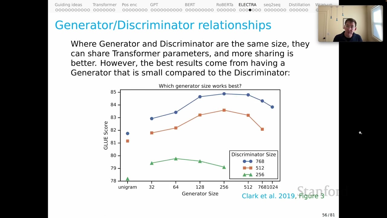
00:02:58.280 | First thing is an observation.
00:02:59.680 | Where the generator and discriminator are the same size, they could, in principle, share
00:03:04.440 | their transformer parameters.
00:03:06.640 | And the team found that more sharing is indeed better.
00:03:09.800 | However, the best results come from having a generator that is small compared to the
00:03:15.640 | discriminator, which means less sharing.
00:03:18.880 | Here's a chart summarizing their evidence for this.
00:03:21.560 | Along the x-axis, I have the generator size going up to 1024.
00:03:26.760 | And along the y-axis, we have GLU score, which will be our proxy for overall quality.
00:03:32.880 | The blue line up here is the discriminator at size 768.
00:03:37.000 | And we're tracking different generator sizes, as I said.
00:03:39.720 | And you see this characteristic reverse U-shape, where, for example, the best discriminator
00:03:44.940 | at size 768 corresponds to a generator of size 256.
00:03:50.320 | And indeed, as the generator gets larger and even gets larger than the discriminator, performance
00:03:55.800 | drops off.
00:03:57.220 | And that U-shape is repeated for all these different discriminator sizes, suggesting
00:04:02.000 | a real finding about the model.
00:04:04.000 | I think the intuition here is that it's kind of good to have a small and relatively weak
00:04:08.680 | generator so that the discriminator has a lot of interesting work to do, because after
00:04:13.560 | all, the discriminator is our focus.
00:04:18.160 | The paper also includes a lot of efficiency studies.
00:04:20.880 | And those, too, are really illuminating.
00:04:22.780 | This is a summary of some of their evidence.
00:04:25.200 | Along the x-axis, we have pre-trained flops, which you can think of as a raw amount of
00:04:30.000 | overall compute needed for training.
00:04:32.880 | And along the y-axis, again, we have the GLUE score.
00:04:36.200 | The blue line at the top here is the full Elektra model.
00:04:39.040 | And the core result here is that for any compute budget you have, that is any point along the
00:04:43.480 | x-axis, Elektra is the best model.
00:04:47.140 | It looks like in second place is adversarial Elektra.
00:04:50.400 | That's an intriguing variation of the model, where the generator is actually trained to
00:04:55.000 | try to fool the discriminator.
00:04:57.180 | That's a clear intuition that turns out to be slightly less good than the more cooperative
00:05:01.680 | objective that I presented before.
00:05:04.860 | And then the green lines are intriguing as well.
00:05:06.720 | So for the green lines, we begin by training just in a standard BERT fashion.
00:05:12.400 | And then at a certain point, we switch over to the full Elektra model.
00:05:16.320 | And what you see there is that in switching over to full Elektra, you get a gain in performance
00:05:21.720 | for any compute budget relative to the standard BERT training continuing as before, which
00:05:26.880 | is the lowest line in the chart.
00:05:29.940 | So a clear win for Elektra relative to these interesting competitors.
00:05:35.220 | And they did further efficiency analyses.
00:05:38.400 | Let me review some of what they found there.
00:05:40.360 | This is the full Elektra model as I presented it before.
00:05:44.340 | We could also think about Elektra 15%.
00:05:47.440 | And this is the case where for the discriminator, instead of having it make predictions about
00:05:52.160 | all of the input tokens, we just zoom in on the tokens that were part of this x corrupt
00:05:58.240 | sequence, ignoring all the rest.
00:05:59.920 | That's a very BERT-like intuition where the ones that matter were these ones that got
00:06:04.360 | masked down here.
00:06:06.400 | That makes fewer predictions for the discriminator.
00:06:10.360 | Replace MLM is where we use the generator with no discriminator.
00:06:16.040 | This is a kind of ablation of BERT.
00:06:18.160 | And then all tokens MLM is a kind of variant of BERT where instead of turning off the objective
00:06:23.360 | for some of the items, we make predictions about all of them.
00:06:27.840 | And here's a summary of the evidence that they found in favor of Elektra.
00:06:31.680 | That's at the top here, according to the Glue score.
00:06:34.480 | All tokens MLM and replace MLM, those BERT variants are just behind.
00:06:39.360 | And that's sort of intriguing because it shows that even if we stick to the BERT architecture,
00:06:44.220 | we could have done better simply by making more predictions than BERT was making initially.
00:06:51.560 | Behind those is Elektra 15%.
00:06:53.820 | And that shows that on the discriminator side, again, it pays to make more predictions.
00:06:58.840 | If we retreat to the more BERT-like mode where we predict only for the corrupted elements,
00:07:03.740 | we find that performance degrades.
00:07:06.240 | And then at the bottom of this list is the original BERT model showing a clear win overall
00:07:11.600 | for Elektra according to this Glue benchmark.
00:07:16.380 | The Elektra team released three models initially, small, base, and large.
00:07:21.020 | Base and large kind of correspond roughly to BERT releases.
00:07:24.100 | And small is a tiny one that they say is designed to be quickly trained on a single GPU.
00:07:29.300 | Again, another nod toward increasing emphasis on efficiency for compute as an important
00:07:35.560 | ingredient in research in this space.
00:07:37.720 | Thanks.
00:07:38.720 | [END OF TRANSCRIPT]
00:07:38.740 | [BLANK_AUDIO]