"Decrappify" at Facebook F8 - New Approaches to Image and Video Reconstruction Using Deep Learning

00:00:00.000 | I want to thank all of you for your time and for your time.

00:00:05.000 | Thank you.

00:00:07.000 | >> Hi, thanks for coming, everybody.

00:00:16.000 | There's a few seats at the front still if you're standing at the

00:00:19.000 | back, by the way.

00:00:21.000 | Some over here as well.

00:00:23.000 | Hi, my name is Jeremy Howard, and I am going to be talking to

00:00:29.000 | you about fast AI.

00:00:31.000 | I'm from fast AI.

00:00:34.000 | You may know of us from our software library called

00:00:37.000 | excitingly enough, fast AI, which sits on top of PyTorch

00:00:41.000 | and powers some of the stuff you'll be seeing here today.

00:00:45.000 | You may also know of us from our course, course.fast.ai,

00:00:49.000 | which has taught hundreds of thousands of people deep

00:00:51.000 | learning from scratch.

00:00:53.000 | Our first part of our course out now covers all of these

00:00:56.000 | concepts, and I'll tell you more about the upcoming new course

00:01:00.000 | later this afternoon.

00:01:02.000 | Our course covers many topics.

00:01:06.000 | Each one, there's a video, there's lesson notes,

00:01:09.000 | there's a community of tens of thousands of people learning

00:01:12.000 | together, and one of the really interesting parts of the last

00:01:16.000 | course was lesson seven, which, amongst other things,

00:01:20.000 | covered generative networks.

00:01:22.000 | And in this lesson, we showed this particular technique.

00:01:27.000 | This here is a regular image, and this here is a crapified

00:01:34.000 | version of this regular image.

00:01:36.000 | And in this technique that we taught in lesson seven of the

00:01:39.000 | course, we showed how you can generate this from this in some

00:01:45.000 | simple, heuristic manner.

00:01:47.000 | So in this case, I down sampled the dog.

00:01:50.000 | I added JPEG artifacts, and I added some random obscuring

00:01:55.000 | text.

00:01:57.000 | So once you've done that, it's then a piece of cake to use

00:02:00.000 | PyTorch and fast.ai to create a model that goes in the other

00:02:07.000 | direction.

00:02:08.000 | So it can go in this direction in a kind of deterministic,

00:02:11.000 | heuristic manner, but to go from here to here is obviously

00:02:15.000 | harder, because you have to, like, figure out what's actually

00:02:18.000 | being obscured here, and what are the JPEG artifacts actually

00:02:21.000 | hiding, and so forth.

00:02:23.000 | So that's why we need to use a deep learning neural network to

00:02:27.000 | do that process.

00:02:28.000 | So here's the cool thing.

00:02:30.000 | You can come up with any heuristic crapification function

00:02:34.000 | you like, which is a deterministic process, and then

00:02:38.000 | train a neural network to do the opposite, which allows you to

00:02:42.000 | do almost anything you can imagine in terms of generative

00:02:46.000 | imaging.

00:02:47.000 | So, for example, in the course, we showed how that exact

00:02:50.000 | process, when you then apply it to this crappy JPEG low

00:02:55.000 | resolution cat, turned it into this beautiful high resolution

00:03:01.000 | image.

00:03:02.000 | So this process does not require giant clusters of computers

00:03:10.000 | and huge amounts of labeled data.

00:03:12.000 | In this case, I used a small amount of data trained for a

00:03:16.000 | couple of hours on a single gaming GPU to get a model that

00:03:23.000 | can do this.

00:03:24.000 | And once you've got the model, it takes a few milliseconds to

00:03:28.000 | convert an image.

00:03:29.000 | So it's fast, it's effective, and so when I saw this come out

00:03:36.000 | of this model, I was like -- I was blown away.

00:03:40.000 | How many people here have heard of GANs, or Generative

00:03:43.000 | Adversarial Networks?

00:03:44.000 | This has no GANs.

00:03:47.000 | GANs are famously difficult to train.

00:03:50.000 | They take a lot of time, a lot of data, a lot of compute.

00:03:54.000 | This simple approach requires no GANs at all.

00:03:57.000 | I was then amazed at about the time that I was building this

00:04:01.000 | lesson when I started seeing pictures like this online from

00:04:05.000 | something called Deoldify, which takes black and white images

00:04:11.000 | and converts them into full-color images.

00:04:14.000 | These are actual historical black and white images I'm going

00:04:17.000 | to show you.

00:04:18.000 | So this was built by a guy called Jason, who you're about to

00:04:21.000 | hear from, who built this thing called Deoldify.

00:04:23.000 | I reached out to him and I discovered he's actually a fast

00:04:26.000 | AI student himself.

00:04:27.000 | He had been working through the course, and he had kind of

00:04:30.000 | independently invented some of these decrapification approaches

00:04:34.000 | that I had been working on, but he had kind of gone in a

00:04:38.000 | slightly different direction as well.

00:04:40.000 | And so we joined forces, and so now we can show you the results

00:04:45.000 | of the upcoming new version of Deoldify to be released today,

00:04:49.000 | which includes all of the stuff from the course I just

00:04:52.000 | described and a bunch of other stuff as well, and it can create

00:04:56.000 | amazing results like this.

00:04:58.000 | Check this out.

00:04:59.000 | Here is an old black and white historical photo where you can

00:05:04.000 | kind of see there's maybe some wallpaper and there's some kind

00:05:08.000 | of dark looking lamp, and the deep learning neural network has

00:05:11.000 | figured out how to color in the plants and how to add all of the

00:05:15.000 | detail of the seat and maybe what the wallpaper actually

00:05:18.000 | looks like and so forth.

00:05:20.000 | It's like an extraordinary job because this is what a deep

00:05:24.000 | learning network can do.

00:05:25.000 | It can actually use context and semantics and understanding of

00:05:29.000 | what are these images and what might they have looked like.

00:05:34.000 | Now that is not to say it knows really what they look like, and

00:05:37.000 | sometimes you get really interesting situations like this.

00:05:40.000 | Here is the Golden Gate Bridge under construction in 1937, and

00:05:46.000 | it looks here like it might be white.

00:05:51.000 | And the model made it white.

00:05:55.000 | Now, the truth is this might not be historically accurate or it

00:06:00.000 | might be we actually don't know, right?

00:06:03.000 | So actually Jason did some research into this and discovered

00:06:06.000 | at this time apparently they had put some kind of red primer to

00:06:12.000 | see what it would look like, and it was a lead-based paint, and

00:06:15.000 | we don't know in the sunlight did it look like this or not.

00:06:19.000 | So historical accuracy is not something this gives us, and

00:06:23.000 | sometimes historical accuracy is something we can't even tell

00:06:27.000 | because there aren't color pictures of this thing, right?

00:06:31.000 | So it's an artistic process, it's not a historical reenactment

00:06:36.000 | process, but the results are amazing.

00:06:39.000 | You look at tiny little bits like this and you zoom in and you

00:06:43.000 | realize it actually knows how to color in porcelain.

00:06:46.000 | It's extraordinary what a deep learning network can do from

00:06:51.000 | the simple process of crappification and decrappification.

00:06:55.000 | So in this case the crappification was take a color

00:06:58.000 | image, make it black and white, randomly screw up the contrast,

00:07:02.000 | randomly screw up the brightness, then try and get it to

00:07:05.000 | undo it again just using standard images and then apply it

00:07:10.000 | to classic black and white photos.

00:07:14.000 | So then one of my colleagues at the Wicklow AI Medical

00:07:19.000 | Research Initiative, a guy named Fred Munro, said we should go

00:07:26.000 | visit the Salk Institute because at the Salk Institute they're

00:07:29.000 | doing amazing stuff with $1.5 million electron microscopes

00:07:34.000 | that create stuff like this.

00:07:37.000 | And these little dots are the things that your neurotransmitters

00:07:41.000 | flow through.

00:07:43.000 | And so there's a crazy guy named Uri at Salk who's sitting over

00:07:47.000 | there who's trying to use these things to build a picture of

00:07:51.000 | your whole brain.

00:07:53.000 | And this is not a particularly easy thing to do.

00:07:55.000 | And so they try taking this technique and crappifying high

00:07:59.000 | resolution microscopy images and then turning them back again

00:08:03.000 | into the original high res and then applying it to this, this

00:08:08.000 | is what comes out.

00:08:10.000 | And so you're going to hear from both of these guys about the

00:08:12.000 | extraordinary results because they've gone way beyond even

00:08:15.000 | what I'm showing you here.

00:08:17.000 | But the basic approach is pretty simple.

00:08:19.000 | You can use fast AI built on top of PyTorch to grab pretty much

00:08:24.000 | any data set with one line of code or four lines of code

00:08:28.000 | depending on how you look at it using our data blocks API which

00:08:31.000 | is by far the most flexible system for getting data to deep

00:08:36.000 | learning of any library in the world.

00:08:39.000 | Then you can use our massive fast AI dot vision library of

00:08:42.000 | transforms to very quickly create all kinds of augmentations.

00:08:46.000 | And this is where the crappification process can come in.

00:08:49.000 | You can add your JPEG artifacts or your black and white or

00:08:52.000 | rotators or brightness or whatever.

00:08:56.000 | And then on top of that, you then can take that crappified

00:09:00.000 | picture and put it through a unit.

00:09:04.000 | Who here has heard of a unit before?

00:09:06.000 | So a unit is a classic neural network architecture which takes

00:09:10.000 | a high input image, pulls out semantic features from it and

00:09:14.000 | then upsizes it back again, generates some image.

00:09:18.000 | And units were incredibly powerful in the biomedical

00:09:23.000 | bioimaging literature.

00:09:25.000 | And in medical imaging, they've changed the world.

00:09:28.000 | They're rapidly moving to other areas as well.

00:09:31.000 | But at the same time, lots of other techniques have appeared

00:09:35.000 | in the broader computer vision literature that never made

00:09:38.000 | their way back into units.

00:09:40.000 | So what we did in fast AI was we actually incorporated all of

00:09:45.000 | the state-of-the-art techniques from up sampling.

00:09:49.000 | There's something called pixel shuffle.

00:09:51.000 | We're removing checkerboard artifacts.

00:09:52.000 | There's something called learnable blur.

00:09:54.000 | For normalization, there's something called spectral norm.

00:09:56.000 | There's a thing called a self-attention layer.

00:09:58.000 | We put it all together.

00:09:59.000 | So in fast AI, if you say, "Give me a unit loader," it does

00:10:04.000 | the whole thing for you.

00:10:05.000 | And you get back something that's actually not just a

00:10:08.000 | state-of-the-art network but contains a bunch of stuff that

00:10:11.000 | can be put together even in the academic literature.

00:10:15.000 | And so the results of this are fantastic.

00:10:17.000 | But of course, the first thing you need to do is to train a model.

00:10:20.000 | So with the fast AI library, when you train a model, you say,

00:10:24.000 | "Fit one cycle," and it uses, again, the best state-of-the-art

00:10:28.000 | mechanism for training models in the world, which it turns out

00:10:31.000 | is a very particular kind of learning rate annealing and a

00:10:35.000 | very particular kind of momentum annealing, something called

00:10:38.000 | one-cycle training from amazing researcher named Leslie Smith.

00:10:42.000 | So you put all this stuff together.

00:10:47.000 | You need one more step, which is you need a loss function.

00:10:50.000 | And so the key thing here that allows us to get these great

00:10:54.000 | results without a gain is that we've, again, stolen other

00:10:58.000 | stuff from the neural network literature, which is there's

00:11:01.000 | something called Graham loss that was used for generating

00:11:06.000 | artistic pictures.

00:11:08.000 | And we basically combine that with what's called feature loss

00:11:14.000 | together with some other cool techniques to create this really

00:11:18.000 | uniquely powerful loss function that we show in the course.

00:11:22.000 | So now we've got the CRAPified data.

00:11:25.000 | We've got the loss function.

00:11:27.000 | We've got the architecture.

00:11:28.000 | We've got the training schedule.

00:11:30.000 | And you put it all together, and you get really beautiful results.

00:11:34.000 | And then if you want to, you can then add on at the very end

00:11:38.000 | a gain.

00:11:40.000 | But we have a very cool way of doing gains, which is we've

00:11:43.000 | actually figured out how to train a gain on a pre-trained model.

00:11:48.000 | So you can do all the stuff you've just seen and then add

00:11:51.000 | a gain just at the very end, and it takes like an hour or two

00:11:55.000 | of extra training.

00:11:56.000 | We actually found for the stuff we were doing for super

00:11:59.000 | resolution, we didn't really need the gain.

00:12:01.000 | It actually didn't help.

00:12:03.000 | So we just used an hour or two of regular unit training.

00:12:07.000 | But what then Jason did was he said, OK, that's nice.

00:12:14.000 | But what if we went way, way, way, way, way further?

00:12:17.000 | And so I want to show you what Jason managed to build.

00:12:20.000 | Jason?

00:12:21.000 | Thanks, Jeremy.

00:12:28.000 | So with the Oldified Success and SEAL images, the next logical

00:12:33.000 | step in my mind was, well, what about moving images?

00:12:36.000 | Can we make that work as well, a.k.a. video?

00:12:39.000 | And the answer turned out to be a resounding yes.

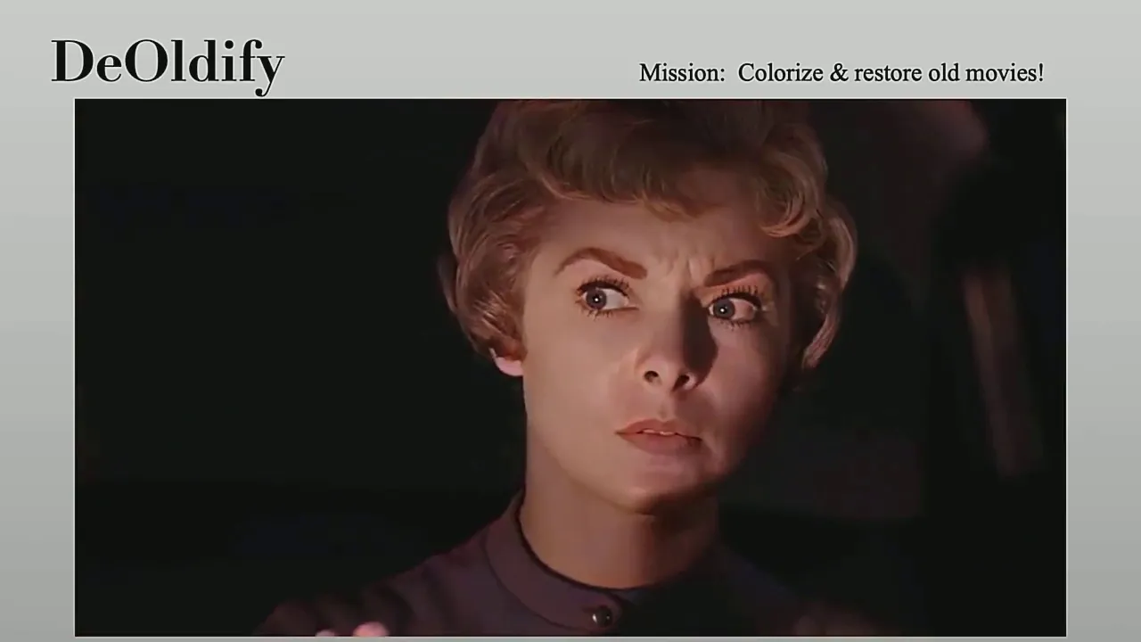
00:12:43.000 | So for the first time publicly, I'm going to show you what the

00:12:47.000 | Oldified video looks like.

00:12:50.000 | [VIDEO PLAYBACK]

00:12:51.000 | -You better get on the job.

00:13:16.000 | Some of the kids may be up this afternoon.

00:13:18.000 | -Oh, Jack, we can get along without dragging those young

00:13:21.000 | kids up here.

00:13:22.000 | -Oh, why don't you button up your lip?

00:13:24.000 | You're always squawking about something.

00:13:25.000 | You got more static on the radio.

00:13:27.000 | [END PLAYBACK]

00:13:33.480 | [MUSIC PLAYING]

00:13:53.440 | So that's the Oldified video.

00:13:56.480 | So now I'm going to tell you how that video was made.

00:14:05.120 | So it turns out, if you want great video, you actually have

00:14:08.200 | to focus on great images.

00:14:10.160 | And that is really composed of three key approaches.

00:14:15.400 | The first is reliable feature detection, the second is

00:14:18.640 | self-attention, and the third is a new GAN training technique

00:14:22.720 | that we've been collaborating on with Fast AI that I'm really

00:14:25.600 | excited about.

00:14:27.920 | So first is reliable feature detection.

00:14:30.280 | So the most obvious thing to do with a generator that's

00:14:35.120 | unit-based, if you want to make it better, is to use a

00:14:38.760 | bigger ResNet backbone.

00:14:40.720 | So instead of using ResNet 34, we use ResNet 101 in this

00:14:44.120 | case, and that allows the generator to pick up on

00:14:48.960 | features better.

00:14:51.600 | The second thing, though, and this is possibly even more

00:14:55.440 | important, is you need to acknowledge the fact that

00:14:58.200 | you're dealing with old and grainy film.

00:15:01.720 | So what you need to do is you need to

00:15:04.240 | simulate that condition.

00:15:06.240 | And so you do lots of augmentation with brightness

00:15:09.520 | and contrast and Gaussian noise to simulate film grain.

00:15:16.000 | And if you get this right, that means you're going to have

00:15:19.400 | less problems with colorization, because the

00:15:21.280 | features are going to be detected correctly.

00:15:23.360 | If you get it wrong, I'll point this out.

00:15:26.920 | You get things like this, this zombie hand right here on the

00:15:29.800 | door frame.

00:15:31.640 | And it's pretty unsightly.

00:15:32.880 | The second thing is self-attention.

00:15:37.640 | So normal convolutional networks with their individual

00:15:42.160 | convolutions, they're focusing on small areas of the image at

00:15:46.960 | any one time.

00:15:47.760 | It's called their receptive field.

00:15:49.880 | And that can be problematic if you're making a colorization

00:15:53.440 | model based on that alone, because those convolutions are

00:15:57.240 | not going to know what's going on on the left side versus the

00:16:01.040 | right side of the image.

00:16:02.320 | So as a result, in this case, you get a different color to

00:16:07.280 | the ocean here versus here versus here.

00:16:12.200 | Whereas on the de-oldify model, we use self-attention.

00:16:15.080 | Self-attention allows for features on the global scale to

00:16:19.120 | be taken into account.

00:16:21.480 | And you can see that the ocean on the right side there, the

00:16:24.760 | right side render, is consistently colored in.

00:16:28.280 | I like that, too.

00:16:35.120 | So the next thing, GAN.

00:16:36.840 | So the original de-oldify uses GANs.

00:16:41.320 | And the reason why it went for GANs is because they're

00:16:44.560 | really good at generating realism.

00:16:46.600 | They're uniquely good at generating realism, really.

00:16:50.720 | And my problem was I didn't know how to write a loss

00:16:54.400 | function that would properly evaluate whether or not

00:16:58.120 | something is realistically colored or not.

00:17:00.680 | I tried.

00:17:02.000 | I tried to do not GANs because they're kind of a pain.

00:17:05.600 | But anyway, so the reason why de-oldify has great

00:17:12.360 | colorization is because of GANs.

00:17:14.280 | The original had great colorization because of that.

00:17:16.840 | But there's a big drawback.

00:17:20.320 | First, they're really slow.

00:17:23.040 | The original de-oldify took like three to five days to

00:17:25.520 | train on my home PC.

00:17:29.360 | But the second thing is that they're really unstable.

00:17:32.720 | So the original de-oldify, while it had great renders, if

00:17:38.360 | you, quite frankly, cherry-picked after a few trials,

00:17:44.160 | overall, you'd still get a lot of glitchy results.

00:17:47.360 | And you'd have unsightly discoloration.

00:17:50.800 | And that was because of the GAN instability

00:17:52.640 | for the most part.

00:17:54.560 | And then finally, they're just really difficult to get

00:17:56.560 | right, hyperparameters you have to tune.

00:17:59.600 | And experiment after experiment.

00:18:01.440 | I probably did over 1,000 experiments before I actually

00:18:04.000 | got it right.

00:18:06.060 | So the solution we arrived at was actually to just almost

00:18:11.080 | avoid GANs entirely.

00:18:12.600 | So we're calling that no-GAN.

00:18:14.680 | So there's three steps to this.

00:18:17.480 | First, you pre-train the generator without GAN.

00:18:20.920 | And you're doing this the vast majority of the time.

00:18:24.480 | In this case, we're using what Jeremy mentioned earlier,

00:18:26.800 | which was feature loss or perceptual loss.

00:18:29.400 | That gets you really far.

00:18:31.560 | But it's still a little dull up to that point.

00:18:35.320 | The second step is you want to pre-train the critic

00:18:38.620 | without GAN, again, as a binary classifier.

00:18:41.880 | So you're doing a binary classification

00:18:44.840 | on those generated images from that first step

00:18:48.640 | and the real images.

00:18:51.140 | And finally, the third step is you

00:18:53.200 | take those pre-generated components

00:18:56.360 | and you're training them together as GAN.

00:18:58.280 | Finally, but only briefly.

00:19:00.600 | This is really brief.

00:19:01.800 | It's only 30, 90 minutes for de-oldify.

00:19:04.800 | And put that in perspective, you see

00:19:07.840 | this graph on the bottom here?

00:19:10.000 | That orange-yellow part, that's the actual GAN training part.

00:19:14.780 | The rest of that is pre-training.

00:19:17.880 | But the great thing about this is in the process,

00:19:20.940 | you get essentially the benefits of GANs

00:19:24.520 | without disability problems that I just described.

00:19:29.640 | So now I'm going to show you what this actually looks like,

00:19:32.320 | starting from a completed pre-generated generator

00:19:37.800 | and then running that through the GAN portion of no GAN.

00:19:41.520 | And I'm actually going to take you a little too far,

00:19:43.600 | because I want you to see where it looks good

00:19:47.160 | and then where it gets a little too much GAN.

00:19:50.360 | So this is before GAN.

00:19:54.120 | This is where you pre-train it.

00:19:55.800 | It's a little dull at this point.

00:19:58.040 | Here you can already see colors being introduced.

00:20:00.040 | This is like minutes in the training.

00:20:02.480 | Right here is actually where you want to stop.

00:20:04.520 | No, it doesn't look too bad yet, but you're

00:20:10.200 | going to start seeing their orange skin.

00:20:13.440 | Or their skin's going to turn orange, rather.

00:20:17.160 | Yeah, right here.

00:20:18.040 | So you don't want that.

00:20:19.480 | You might be surprised.

00:20:23.560 | So the stopping point of no GAN training at that GAN part

00:20:29.880 | is right in the middle of the training loss going down,

00:20:33.400 | which is kind of counterintuitive.

00:20:35.320 | And I've got to be clear on this.

00:20:38.040 | We haven't put a paper out on this.

00:20:39.640 | I don't know why that is, honestly.

00:20:43.760 | I think it might be because of stability issues.

00:20:47.480 | The batch size I was using back there was only five,

00:20:51.120 | which is kind of cool.

00:20:52.000 | I mean, it seems like no GAN accommodates low batch size

00:20:55.840 | really nicely.

00:20:57.040 | It's really surprising it turns out as good as it does.

00:21:00.280 | But yeah, that's where I'm actually stopping it.

00:21:05.680 | So no GAN really solved my problems here.

00:21:09.320 | And I think this illustrates it pretty clearly.

00:21:11.900 | So when we made video with the original Deolify,

00:21:15.680 | it looked like this on the left.

00:21:17.120 | And you can see their clothing is flashing red.

00:21:20.720 | And the guy's hand has got a fireball forming on it.

00:21:24.520 | It wasn't there in the original.

00:21:27.160 | Whereas on the right side, with a no GAN training,

00:21:30.680 | you see all those problems just disappear.

00:21:32.440 | It's just so much cleaner.

00:21:34.000 | Now, you might be wondering if you

00:21:38.760 | can use no GAN for anything else besides colorization.

00:21:41.600 | It's a fair question.

00:21:42.780 | And the answer is yes.

00:21:44.660 | We actually tried it for super resolution as well.

00:21:48.600 | So I just took Jeremy's lesson on this with the feature loss.

00:21:54.880 | Which got it up to that point on the left.

00:21:58.040 | I plot no GAN on the results, and ran it for like 15 minutes,

00:22:04.320 | and got those results on the right, which are, I think,

00:22:07.420 | noticeably sharper.

00:22:08.240 | There's a few more things to talk about here that I think

00:22:12.720 | are interesting.

00:22:14.040 | First is that super resolution result

00:22:19.480 | you saw on the previous slide.

00:22:21.200 | That was produced by using a pre-trained critic

00:22:23.640 | on colorization.

00:22:24.360 | So I just reused the critic that I used for colorization,

00:22:28.760 | and fine-tuned it, which is a lot less effort, and it worked.

00:22:34.480 | That's really useful.

00:22:36.200 | Second thing is there was absolutely no temporal modeling

00:22:40.120 | used for making these videos.

00:22:43.360 | It's just image to image.

00:22:45.600 | It's literally just what we do for normal photos.

00:22:48.480 | So I'm not changing the model at all in that respect.

00:22:53.000 | And then finally, this can all be done on a gaming PC,

00:22:58.840 | just like Jeremy was talking about.

00:23:01.600 | In my case, I was just running all this stuff on a 1080 Ti

00:23:04.800 | for any one run.

00:23:06.520 | So I hope you guys find no GAN useful.

00:23:09.960 | We certainly did.

00:23:10.840 | It solved so many of the problems we had.

00:23:14.600 | And I'm really happy to announce to you guys

00:23:16.960 | that it's up on GitHub, and you can try it out now.

00:23:19.760 | And there's Colab notebooks.

00:23:21.200 | So please enjoy.

00:23:22.880 | And next up is Dr. Manner.

00:23:26.320 | He's going to talk about his awesome work at Salk Institute.

00:23:30.280 | [APPLAUSE]

00:23:32.240 | Hi, everyone.

00:23:38.400 | My name is Uri Manner.

00:23:39.640 | I'm the director of the Weight Advanced Biophotonics

00:23:42.600 | Core at the Salk Institute for Biological Studies.

00:23:46.680 | How many of you know what the Salk Institute is?

00:23:49.640 | All right, for those of you who don't know,

00:23:52.120 | it's a relatively small biological research

00:23:55.560 | institute, as per its name.

00:23:56.760 | It was founded by Jonas Salk in 1960.

00:23:59.920 | He's the one who created the polio vaccine, which fortunately

00:24:04.120 | we don't have to worry about today.

00:24:05.480 | And it's relatively small.

00:24:09.520 | It has about 50 labs, which may sound like a lot to you,

00:24:12.240 | but just to put things in perspective,

00:24:14.480 | in comparison to a state university, for example,

00:24:17.440 | a single department might have that many labs.

00:24:20.640 | So it's relatively small, but it's incredibly mighty.

00:24:24.120 | Every single lab is run by a world-class leader

00:24:28.040 | in their field.

00:24:30.120 | And not only is it cutting edge and small, but powerful.

00:24:36.040 | It's also broad.

00:24:37.680 | So we have people studying cancer research,

00:24:41.360 | neurodegeneration and aging, and even plant research.

00:24:46.680 | And our slogan is, where cures begin.

00:24:50.400 | Because we are not a clinical research institute.

00:24:52.680 | We are interested in understanding

00:24:54.440 | the fundamental mechanisms that underlie life.

00:24:58.120 | And the idea is that in order to fix something,

00:25:00.400 | you have to know how it works.

00:25:02.160 | So by understanding the basic mechanisms that drive life,

00:25:05.400 | and therefore disease, we have a chance at actually fixing it.

00:25:10.000 | So we do research on cancer, like I mentioned,

00:25:13.400 | neurodegeneration.

00:25:15.000 | And even plant research, you could think of as a cure.

00:25:18.320 | For example, my colleagues have calculated

00:25:20.840 | that if we could increase the carbon capture capabilities

00:25:24.720 | of all the plants on the planet by 20%,

00:25:28.440 | we could completely eradicate all of the carbon emissions

00:25:31.000 | of the human race.

00:25:33.080 | So we have a study going on right now

00:25:34.880 | where we're classifying the carbon capturing

00:25:37.680 | capabilities of plants from all over the globe,

00:25:39.720 | from many different climates, to try

00:25:41.680 | to understand how we can potentially

00:25:43.200 | engineer or breed plants that could do a better

00:25:45.280 | job of capturing carbon.

00:25:47.560 | And that's just, of course, one small example

00:25:49.520 | of what we're doing at the Salk Institute.

00:25:51.880 | Now, as a director of the Weight Advanced Biophotonics

00:25:54.920 | Core, my job is to make sure that all of the researchers

00:25:58.280 | at the Salk have the most cutting edge, highly capable

00:26:01.960 | imaging equipment, microscopy, which is pretty much synonymous

00:26:06.520 | with biology.

00:26:07.760 | So I get to work with all of these amazing people,

00:26:09.920 | and it's an amazing job.

00:26:12.080 | And so I'm always looking for ways

00:26:15.960 | to improve our microscopes and improve our imaging.

00:26:20.280 | As a microscopist, I have been plagued

00:26:23.400 | by this so-called eternal triangle of compromise.

00:26:26.480 | Are any of you photographers?

00:26:28.560 | Have any of you ever worked with a manual SLR camera?

00:26:32.440 | So you're familiar with this triangle of compromise.

00:26:34.960 | If you want more light, you have to use a slower shutter speed,

00:26:38.720 | which means that you're going to get motion blur.

00:26:41.520 | If you want higher resolution, you

00:26:43.400 | have to make compromises in your adaptive focus.

00:26:46.640 | Or you have to use a higher flash.

00:26:49.240 | And all of these principles apply to microscopy as well,

00:26:51.960 | except we don't use a flash.

00:26:53.680 | We use electrons, or we use photons.

00:26:57.040 | And a lot of times, we're trying to image live samples,

00:26:59.520 | live cells, and I'll show you soon what that looks like.

00:27:04.240 | You may be surprised, but our cell

00:27:06.220 | did not evolve to have lasers shining on them.

00:27:09.240 | So if you use too many photons, if you

00:27:10.880 | use too high of a laser power, too high of a flash,

00:27:13.920 | you're going to cook the cells.

00:27:15.560 | And we're trying to study biology, not culinary science.

00:27:18.880 | So we need to use fewer photons when

00:27:20.600 | we're trying to image normal physiological processes.

00:27:24.160 | If you're trying to image cells under stress,

00:27:25.920 | then maybe using more photons is a way to do that.

00:27:29.720 | And of course, we care about speed.

00:27:31.220 | We want to capture the dynamic changes.

00:27:33.500 | The whole point of imaging is that if we

00:27:35.560 | have the spatial temporal dynamics, the ultra

00:27:38.080 | structure, the architecture of the system

00:27:40.560 | that underlie life, that underlie ourselves, our tissues,

00:27:43.960 | then we can really understand how they work.

00:27:46.680 | So we want to be able to image all the detail we can

00:27:49.480 | with all the signal to noise that we

00:27:50.960 | can with minimal perturbations.

00:27:54.840 | Now, one of the most popular kinds of microscopes

00:27:57.480 | in my lab and many others is something

00:27:59.600 | called a point scanning microscope.

00:28:01.520 | And the way it works is you scan pixel by pixel

00:28:04.280 | over the sample, and you build up an image that way.

00:28:07.640 | Now, you can imagine, if you want a higher resolution image,

00:28:10.180 | you need to use smaller pixels.

00:28:12.980 | The smaller the pixel, the fewer the photons

00:28:14.920 | and the fewer the electrons that you can collect.

00:28:17.380 | So it ends up being much slower and much more damaging

00:28:21.040 | to your sample.

00:28:21.920 | The higher the resolution, the more damage to your sample.

00:28:26.080 | All right.

00:28:27.120 | So here's a real world example of what

00:28:29.560 | that might look like in terms of speed.

00:28:33.040 | This is an actual pre-synaptic Bhutan.

00:28:38.040 | And on the left, you can see what

00:28:39.200 | happens with a low resolution scan.

00:28:41.400 | And on the right, you can see a high resolution scan.

00:28:43.760 | You can see that on the left, we're refreshing much faster.

00:28:46.800 | On the right, we're refreshing much slower,

00:28:48.920 | but there's more detail in that image.

00:28:51.120 | This is a direct example or a demonstration of the trade-off

00:28:54.440 | between pixel size and speed.

00:28:57.200 | What you can't see here is this is a two-dimensional image.

00:28:59.700 | This is a 40-nanometer section of brain tissue.

00:29:04.800 | And what we really need, if we want

00:29:06.320 | to image the entire brain, which we do,

00:29:08.480 | we're actually trying to image every single synapse,

00:29:10.680 | every single connection in the entire brain

00:29:13.560 | so we can build up a wiring diagram of how this works

00:29:16.840 | so that maybe we can even build more efficient GPUs.

00:29:20.360 | The brain is actually 50,000 times more efficient

00:29:23.360 | than a GPU.

00:29:25.440 | So Google AI is actually investing in this technology

00:29:28.000 | just because they want to be able to build better computers

00:29:30.500 | and better software.

00:29:31.880 | Anyway, I digress.

00:29:33.480 | The brain is 3D, not 2D.

00:29:35.400 | So how do you do this?

00:29:36.600 | One way is to serially section the brain into 40-nanometer

00:29:39.560 | slices throughout the whole thing.

00:29:41.520 | That is really laborious, really hard.

00:29:44.700 | And then you have to align everything.

00:29:46.800 | So what we did was we invested in a $1.5 million

00:29:49.400 | microscope that has a built-in knife that can image and cut

00:29:53.760 | and image and cut automatically.

00:29:56.920 | And then we can go through the entire brain.

00:30:00.040 | And a lot of people around the world

00:30:01.500 | are using this type of technology

00:30:02.920 | for that exact purpose.

00:30:04.520 | It's not just brain.

00:30:05.360 | We can also go through a tumor.

00:30:06.620 | We can go through plant tissue.

00:30:08.960 | So that brings me to my next problem, sample damage.

00:30:12.400 | If we want that resolution, we have to use more electrons.

00:30:15.720 | And when you start using more electrons in our serial

00:30:17.800 | sectioning device, you start to melt the sample.

00:30:21.040 | And the knife can no longer cut it.

00:30:22.440 | Try cutting melted butter.

00:30:24.400 | You can't get clear sections.

00:30:27.200 | And everything starts to fall apart,

00:30:29.040 | or as Jeremy would say, it starts to fall to crap.

00:30:33.520 | Whereas on the right, with a lower pixel resolution

00:30:35.960 | with lower dose, you can actually

00:30:37.680 | see that we can go and we can section through pretty well.

00:30:40.360 | But you can see the image is much grainier.

00:30:42.200 | We no longer have the level of detail

00:30:43.800 | that we really want to be able to map

00:30:45.840 | all of the fine structure of every single connection

00:30:48.840 | in the brain.

00:30:49.880 | But that is the state of connectomics research

00:30:53.560 | in the world today.

00:30:54.440 | Most people are imaging at that resolution.

00:30:57.640 | But that's not satisfying for me.

00:31:00.640 | So in my other life, I'm a photographer.

00:31:03.800 | And actually, on Facebook, I follow Petapixel.

00:31:07.600 | And I was browsing through Facebook, stalking my friends,

00:31:10.360 | and doing whatever you do on Facebook.

00:31:12.520 | And I came across this article where

00:31:15.420 | they show that you can use deep learning to increase

00:31:18.640 | the resolution of compressed or low resolution photos.

00:31:22.040 | I said, aha, what if we can use the same concept

00:31:25.800 | to increase the resolution of our microscope images?

00:31:30.360 | So this is the strategy that we ended up on.

00:31:34.780 | Previously, I used the same model

00:31:37.200 | that they used here, which was based on GANs, which

00:31:39.360 | you've heard about now.

00:31:40.360 | They're amazing.

00:31:41.800 | Problem with GANs is they can hallucinate.

00:31:43.720 | They're hard to train.

00:31:44.960 | It worked well for some data.

00:31:46.280 | It didn't work well for other data.

00:31:48.120 | Then I was very lucky to meet Jeremy and Fred Monroe.

00:31:52.560 | And together, we came up with a better strategy, which

00:31:55.640 | depends on what we call "crapify."

00:31:58.400 | So we take our high resolution EM images, we crapify them,

00:32:04.100 | and then we run them through our dynamic res unit.

00:32:06.920 | And then we tested it with actual high versus low

00:32:10.280 | resolution images that we took on our microscope

00:32:13.120 | to make sure that our model was fine tuned to work the way we

00:32:15.920 | needed it to work.

00:32:17.840 | And the results are spectacular.

00:32:20.200 | So on the left, you can see a low resolution image.

00:32:22.740 | This is analogous to what we would be imaging when

00:32:25.320 | we're doing our 3D imaging.

00:32:28.000 | And as you can see, the vesicles,

00:32:29.600 | which are about 35 nanometers across,

00:32:32.200 | are barely detectable here.

00:32:33.560 | You can kind of tell where one might be here,

00:32:35.400 | but kind of hard to say.

00:32:37.360 | And in the middle, we have the output of our deep learning

00:32:41.040 | model.

00:32:41.960 | And you can see now we can clearly see the vesicles,

00:32:44.480 | and we can quantify them.

00:32:45.860 | And on the right is a high resolution image.

00:32:48.400 | That's our ground truth.

00:32:50.000 | In my opinion, the model actually

00:32:52.000 | produces better looking data than the ground truth.

00:32:54.480 | And there's a couple reasons for that,

00:32:56.600 | which I'm not going to go into, but one reason

00:32:58.920 | is that our training data was acquired on a better microscope

00:33:01.680 | than our testing data.

00:33:02.600 | So now we can actually do that three view sectioning

00:33:08.200 | at the low resolution that we're stuck with because

00:33:10.440 | of sample damage.

00:33:11.600 | But we can reconstruct it and get high resolution data.

00:33:15.200 | And this applies, as it turns out,

00:33:17.720 | to labs around the world.

00:33:19.960 | This is data from another lab from a different organism,

00:33:23.880 | different sample preparation, and it still works.

00:33:27.680 | And that's bonkers, usually in microscopy

00:33:30.640 | and in a lot of cases in deep learning.

00:33:32.800 | If your training data is acquired in a certain way,

00:33:35.200 | and then your testing data is something completely different,

00:33:37.840 | it just doesn't work.

00:33:38.760 | But in our case, it works really well.

00:33:41.180 | So we're super happy with that.

00:33:42.640 | And what that means is that all the connectomas researchers

00:33:45.060 | in the world who have this low resolution data, exabytes

00:33:49.360 | of data, where they can't see the synaptic vesicles,

00:33:52.240 | the details that actually underlie learning, and memory,

00:33:55.400 | and fine tuning of these connections,

00:33:58.440 | we can apply our model to their data,

00:34:00.240 | and we can rescue all of that information

00:34:02.320 | that they have to throw away for the sake of throughput,

00:34:05.840 | or sample damage, or whatever.

00:34:07.480 | The other thing I'll point out is because the data is

00:34:12.760 | so much cleaner, auto encoders, units,

00:34:15.540 | they intrinsically denoise data.

00:34:18.960 | So because the data is cleaner, we can now

00:34:21.240 | segment out so much easier than we ever could before.

00:34:24.400 | So in this segmentation, we've identified

00:34:26.360 | the ER, mitochondria, presynaptic vesicles,

00:34:30.400 | and it was easier than it ever was before.

00:34:32.200 | So not only do we have better data,

00:34:35.040 | we have better analysis of that data

00:34:38.360 | than we ever hoped to have before.

00:34:40.000 | Of course, even without GANS, you

00:34:46.200 | have to worry about hallucinations, false positives.

00:34:50.680 | So we randomized a bunch of low versus high resolution

00:34:54.320 | versus deep learning output, and we

00:34:57.480 | had two expert humans counting the synaptic vesicles

00:35:01.480 | that they saw in the images, and then we

00:35:04.240 | compared to the ground truth.

00:35:07.880 | And of course, the biggest thing is

00:35:10.080 | that you see a lot less false negatives.

00:35:12.480 | We're able to detect way more presynaptic vesicles

00:35:14.840 | than we could before.

00:35:16.040 | We've gone from 46% to 70%.

00:35:18.440 | That's awesome.

00:35:20.440 | Sorry, we've gone from 43% to 13%.

00:35:24.320 | That's huge, even better than I just said.

00:35:27.000 | But we also have a little bit of an increase in false positives.

00:35:31.000 | We've gone from 11% to 17%.

00:35:34.280 | I'm not actually sure all of those false positives are false.

00:35:37.640 | It's just that we have a limit in what our ground truth data

00:35:40.560 | can show.

00:35:43.160 | But the important thing is that the actual error

00:35:49.920 | between our ground truth data and our deep learning data

00:35:53.920 | is on the same order of magnitude,

00:35:56.240 | on the same level as the error between two humans looking

00:36:00.520 | at the ground truth data.

00:36:02.120 | And I can tell you that there is no software that

00:36:04.200 | can do better than humans right now for identifying

00:36:07.040 | presynaptic vesicles.

00:36:08.680 | So in other words, our deep learning output

00:36:11.320 | is as accurate as you can hope to get anyway, which

00:36:15.200 | means that we can and should be using it in the field right

00:36:18.400 | away.

00:36:21.400 | So I mentioned live imaging and culinary versus biological

00:36:25.920 | science.

00:36:26.960 | So here's a cancer cell.

00:36:28.720 | And we're imaging mitochondria that

00:36:30.800 | have been labeled with a fluorescent dye.

00:36:33.240 | And we're imaging it at maximum resolution.

00:36:35.360 | And what you can see is that the image is becoming

00:36:37.320 | darker and darker, which is a sign of something

00:36:39.920 | we call photobleaching.

00:36:41.440 | That's a big problem.

00:36:42.720 | You can also see that the mitochondria is swelling.

00:36:44.960 | They're getting stressed.

00:36:45.960 | They're getting angry.

00:36:47.280 | We want to study mitochondria when they're not

00:36:49.440 | stressed and angry.

00:36:50.200 | We want to know what's normally happening to the mitochondria.

00:36:53.480 | So this is a problem.

00:36:54.400 | We can't actually image for a long period of time

00:36:56.920 | with high spatial temporal resolution.

00:37:00.760 | So we decided to see if we could apply the same method

00:37:03.840 | for live fluorescence imaging.

00:37:05.720 | So we under sample at the microscope.

00:37:08.700 | And then we use deep learning to restore the image.

00:37:11.280 | And as you can see, it works very, very well.

00:37:15.000 | So this methodology applies to electron microscopy

00:37:17.520 | for connectomics.

00:37:18.760 | It applies to cancer research for live cell imaging.

00:37:21.840 | It is a broad use approach that we're very excited about.

00:37:28.440 | So in conclusion, it works.

00:37:32.520 | And I think there's a lot of exciting things

00:37:34.680 | to look forward to.

00:37:35.560 | We didn't use the no GANS approach.

00:37:38.160 | We didn't use some of the more advanced resonant backbones.

00:37:40.840 | There is so much we can do even better than this.

00:37:43.320 | And that's just so exciting to me.

00:37:46.160 | And I just want to point out quickly

00:37:47.680 | that our AI is dependent on NI, natural intelligence.

00:37:52.120 | And this would not have happened at all without Jeremy,

00:37:55.720 | without Fred, and without Lin-Jing Fang,

00:37:57.840 | who's our image analysis engineer at the Salk Institute.

00:38:01.680 | And I also want to point out that all

00:38:04.000 | of these biological studies are massive efforts that

00:38:07.080 | require a whole lot of people, a whole lot of equipment

00:38:10.200 | that contributed a lot to making this kind of stuff happen.

00:38:14.240 | So with that, I'll hand back over to Jeremy.

00:38:16.080 | And thank you very much.

00:38:17.120 | When we started Fast AI a few years ago,

00:38:27.160 | as a self-funded research and teaching lab,

00:38:31.720 | we really hoped that by putting deep learning

00:38:33.840 | in the hands of domain experts like Uri

00:38:37.320 | that they would create stuff that we had never even heard of,

00:38:41.240 | solve problems we didn't even know existed.

00:38:43.680 | And so it's like beyond thrilling for me

00:38:46.720 | to see now that not only has that happened,

00:38:50.320 | but it's also helped us to help launch the Wycraum AI

00:38:54.800 | Medical Research Initiative.

00:38:57.600 | And with these things all coming together,

00:39:02.920 | we're able to see these extraordinary results,

00:39:05.320 | like Deontify and like PSSR, that's

00:39:12.400 | doing this world-changing stuff, which blows my mind what folks

00:39:19.920 | like Uri and Jason have built.

00:39:25.440 | So what I want to do now is to see more people building

00:39:29.840 | mind-blowing stuff, people like you.

00:39:33.240 | And so I would love it if you go to fast.ai as well,

00:39:40.440 | like these guys did, and start your journey towards learning

00:39:43.920 | about building deep learning neural networks with PyTorch

00:39:47.880 | and the Fast AI library.

00:39:49.760 | And if you like what you see, come back in June

00:39:53.600 | to the fast.ai website.

00:39:55.160 | We'll be launching this, which is Deep Learning

00:39:59.560 | from the Foundations.

00:40:01.080 | It's a new course, which will teach you

00:40:04.400 | how to do everything from creating a high-quality matrix

00:40:08.880 | multiplication implementation from scratch,

00:40:12.040 | all the way up to doing your own version of Deontify.

00:40:17.560 | And so we'll be really excited to show you

00:40:20.920 | how things are built inside the Fast AI library,

00:40:24.280 | how things are built inside PyTorch itself.

00:40:27.640 | We'll be digging into the source code

00:40:30.560 | and looking at the actual academic papers

00:40:34.920 | that those pieces of source code are based on

00:40:38.040 | and seeing how you can contribute to the libraries

00:40:40.360 | yourself, do your own experiments,

00:40:43.000 | and move from just being a practitioner to a researcher

00:40:48.520 | doing stuff like what Jason and Uri have shown you today,

00:40:51.760 | doing stuff that no one has ever done before.

00:40:57.880 | So to learn more about all of these decrapification techniques

00:41:03.760 | you've seen today, also in the next day or two,

00:41:06.800 | there will be a post with a lot more detail about it

00:41:09.280 | on the fast.ai blog.

00:41:11.280 | Check it out there.

00:41:12.640 | Check out Deontify on GitHub, where

00:41:15.720 | you can start playing with the code today,

00:41:17.920 | and you can even run it in free Colab notebooks

00:41:22.360 | that Jason has set up for you.

00:41:24.240 | So you can actually colorize your own movies,

00:41:28.760 | colorize your own photos.

00:41:31.040 | Maybe if grandma's got a great black and white photo

00:41:34.080 | of grandpa that she loves, you could turn it

00:41:36.120 | into a color picture and make her day.

00:41:40.360 | So we've got three minutes for maybe one or two questions,

00:41:44.720 | if anybody has any.

00:41:46.640 | No questions?

00:41:53.440 | OK, oh, one question.

00:41:54.640 | Yes.

00:41:55.120 | It looks like it works very reliably with the coloring.

00:42:04.240 | Of course, there could be mistakes happening.

00:42:07.520 | And what about the ethical side of that,

00:42:10.760 | or changing history kind of a thing?

00:42:15.520 | I mean, this is why we mentioned it's an artistic process.

00:42:19.880 | It's not a recreation.

00:42:21.840 | It's not a reenactment.

00:42:23.440 | And so if you give Granny a picture of grandpa,

00:42:27.880 | and she says, oh, no, he was wearing a red shirt, not

00:42:30.200 | a blue shirt, so be it.

00:42:32.080 | But the interesting thing is that, as Jason mentioned,

00:42:36.280 | there's no temporal component of the Deontify model.

00:42:40.000 | So from frame to frame, it's discovering again and again

00:42:43.200 | that's a blue shirt.

00:42:44.720 | And so we don't understand the science behind this.

00:42:47.880 | But we think there's something encoded in the luminance data

00:42:50.920 | of the black and white itself that's

00:42:52.560 | saying something about what the color actually is.

00:42:56.000 | Because otherwise, it just wouldn't work.

00:42:58.280 | So there needs to be a lot more research done into this.

00:43:01.600 | But it really seems like we might

00:43:06.880 | be surprised to discover how often the colors are actually

00:43:10.400 | correct.

00:43:11.280 | Because somehow, it seems to be able to reverse engineer

00:43:13.960 | what the colors probably would have been.

00:43:17.640 | Even as it goes from camera one to camera two

00:43:20.480 | of the same scene, the actors are still

00:43:22.600 | wearing the same college pants.

00:43:24.960 | And so somehow, it knows how to reverse engineer the color.

00:43:30.800 | Any more questions?

00:43:31.480 | Yes, one over there.

00:43:32.400 | I find the super resolution images really interesting.

00:43:41.160 | So there was one that's showing with the cells.

00:43:43.920 | And how we can make it more detailed

00:43:46.880 | with the details on the cell.

00:43:49.520 | So it was side by side with the ground truth data.

00:43:52.600 | And I'm seeing that the one that's

00:43:53.960 | created by the super resolution is actually--

00:43:57.200 | it's interesting because obviously, it's

00:44:00.040 | a lot better than the crappy version.

00:44:02.000 | But it's untrue on some levels in terms of the cell

00:44:06.320 | walls thickness compared to the ground truth.

00:44:09.520 | So my question is, given that AI is making it more detailed

00:44:14.760 | and making stuff up, basically, how can we use that?

00:44:18.480 | Right.

00:44:18.960 | So that's why Uri and his team did this really fascinating

00:44:23.240 | process of actually checking it with humans.

00:44:25.840 | So as he said, they actually decreased the error rate

00:44:31.640 | very significantly.

00:44:32.600 | So that's the main thing.

00:44:34.120 | Did you want to say more about that?

00:44:35.320 | I think you said basically what I would have said,

00:44:37.560 | which is that we tried to use real biological structures

00:44:41.120 | to quantify the error rate.

00:44:42.840 | And we used an example of a really small biological

00:44:45.080 | structure that you wouldn't be able to see in low,

00:44:47.320 | but you can see in high resolution.

00:44:49.720 | And we found that our error rates were within basically

00:44:52.720 | the gold standard of what we would be getting from our ground

00:44:54.960 | truth data anyway.

00:44:56.160 | I'm not saying it's perfect.

00:44:57.720 | I think it will become better, especially working with Jeremy.

00:45:02.080 | But it's already usable.

00:45:03.480 | But partly, this is coming out of algorithmically speaking.

00:45:07.320 | The loss function can actually encode what the domain expert

00:45:11.520 | cares about.

00:45:12.680 | So you pre-train a network that has a loss function where

00:45:15.840 | that feature loss actually only recognizes something is there

00:45:20.000 | if the domain expert said it was there.

00:45:22.000 | So there are things we can do to actually stop it

00:45:24.760 | from hallucinating things we care about.

00:45:27.800 | Thanks, everybody.

00:45:28.680 | Thanks very much.

00:45:30.480 | [MUSIC PLAYING]

00:45:33.840 | [AUDIO OUT]

00:45:37.200 | [BLANK_AUDIO]

"Decrappify" at Facebook F8 - New Approaches to Image and Video Reconstruction Using Deep Learning

Chapters