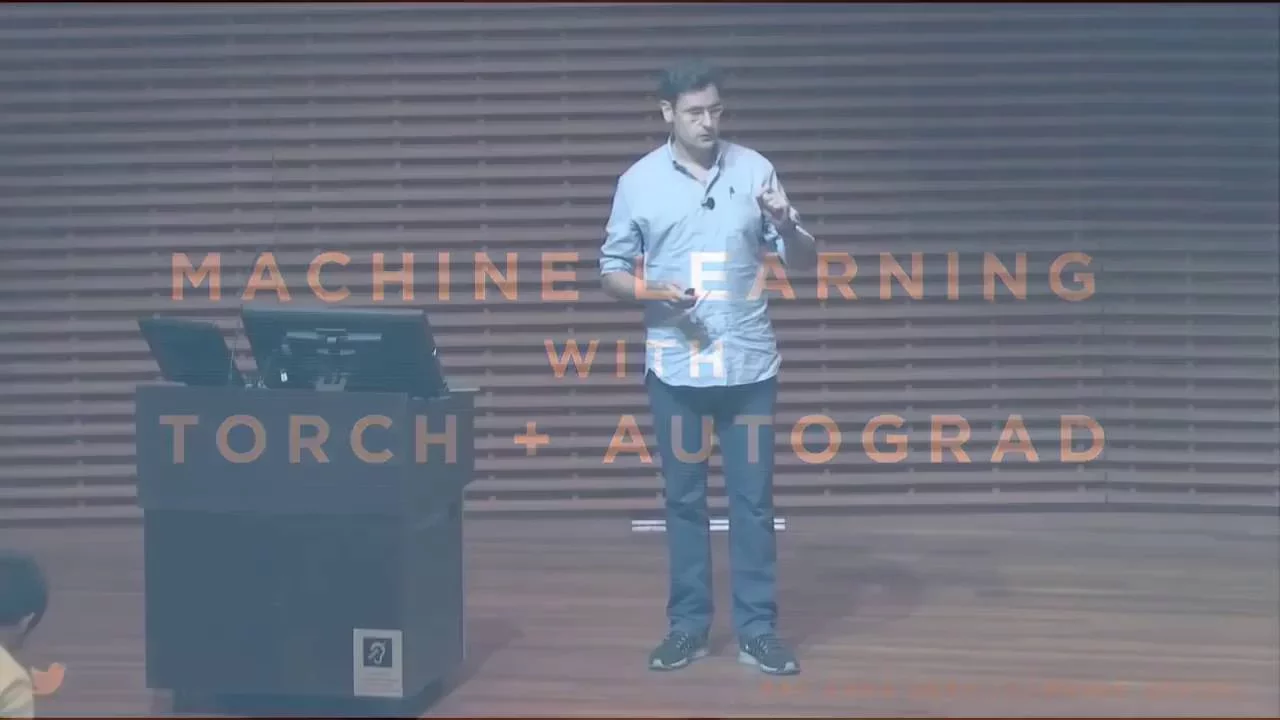
Torch Tutorial (Alex Wiltschko, Twitter)

00:00:00.000 | So I'm going to tell you about machine learning with Torch and with Torch Autograd.

00:00:04.160 | So the description of the talk isn't entirely correct.

00:00:07.880 | I'm going to do practical stuff for the first half.

00:00:11.040 | And then what I want to do is dive into Torch Autograd and some of the concepts that are

00:00:16.180 | behind it.

00:00:17.180 | And those concepts also happen to be shared amongst all deep learning libraries.

00:00:21.540 | So I really want to give you a perspective of the common thread that links all deep learning

00:00:25.920 | software you could possibly use.

00:00:28.200 | And then also talk a bit about what makes each of the libraries different and why there's

00:00:31.400 | -- I will hypothesize why there's so many and the different choices.

00:00:36.920 | So one thing I want to try -- there's been a lot of questions and we've gone over time.

00:00:41.160 | But if there's not questions that go over time in the room, there's a lot of people

00:00:45.160 | watching online.

00:00:46.640 | And if there's extra time, we'll, of course, prioritize people here.

00:00:50.040 | But if you ask a question with the #DLschool hashtag or if you tweet at me directly, I

00:00:54.440 | will try to answer those questions from online and I'll certainly answer them offline as

00:00:58.560 | well.

00:00:59.680 | So ask if you're watching at home.

00:01:02.040 | Maybe that will kind of increase meaningful participation for people watching through

00:01:06.080 | the stream that aren't here today.

00:01:08.480 | A lot of this material was developed with Sumit Chintala at Facebook.

00:01:12.280 | He's kind of the czar of the Torch ecosystem these days.

00:01:16.520 | And Hugo La Rochelle, who you heard from yesterday.

00:01:18.720 | And also Ryan Adams, who's at Twitter with us.

00:01:22.880 | And all this material is available on this GitHub repository that you got actually on

00:01:29.400 | a printed sheet for installing Torch.

00:01:32.800 | So all the examples that I'll show you will be in one notebook.

00:01:36.960 | And then there's a separate notebook, which I actually won't reference in the talk, that's

00:01:39.880 | a full end-to-end walkthrough of how to train a convolutional neural network on CIFAR-10.

00:01:45.840 | So that's kind of a self-paced tutorial notebook that you can work through on your own time.

00:01:49.760 | But I'm going to focus on the basics, on the fundamentals, and hopefully give you some

00:01:54.160 | of the concepts and vocabulary that you can use to really dive into Torch on your own

00:01:58.480 | time.

00:01:59.640 | So let's get going.

00:02:01.080 | So Torch is an array programming language for Lua.

00:02:05.360 | So it's like NumPy, it's like MATLAB, but it's in the Lua language.

00:02:08.880 | So Torch is to Lua, as NumPy is to Python.

00:02:13.160 | So what you can do in Torch, you can do in any language.

00:02:17.080 | This is the absolute minimum basics.

00:02:18.880 | You can grab strings and print them.

00:02:21.560 | You can put things in associative data types.

00:02:24.840 | In Python, there's tuples and lists and sets and dictionaries.

00:02:28.680 | In Lua, there's just one data type called a table.

00:02:32.280 | So you'll see that a lot.

00:02:33.280 | But you can do all those things that I mentioned before with a table.

00:02:36.560 | And you've got for loops and if statements.

00:02:40.360 | The core type of Torch is the tensor.

00:02:43.320 | Just like in NumPy, when you have the nd array, which is a way of shaping sets of numbers

00:02:48.680 | into matrices or tensors, we have the tensor.

00:02:53.200 | And you can fill it up with random numbers.

00:02:54.680 | You can multiply them.

00:02:56.280 | Standard stuff.

00:02:57.280 | But the tensor is the core data type of Torch.

00:03:00.720 | We've got plotting functionality.

00:03:02.680 | Going over at a very high level, I'll show you some more specific code in a moment.

00:03:06.720 | So you can do all the kind of standard stuff that you'd do in any other array-based language.

00:03:12.320 | There's all the tensor functions that you'd like to use, including all the linear algebra

00:03:17.640 | and convolutions and, you know, blast functions.

00:03:21.320 | And I'm leaving this link here.

00:03:22.880 | When the slides get uploaded, you can follow this and kind of dive into the documentation

00:03:26.680 | and see exactly what kind of tools you have at your disposal.

00:03:31.480 | In the notebook, in the itorch notebook, which is something that Sumith put together, you

00:03:36.760 | can prepend any Torch function with a question mark.

00:03:39.320 | And that gives you the help for that function.

00:03:41.760 | So it makes it really nice to discover functionality in the Torch library, in the notebook.

00:03:49.880 | So why is it in Lua?

00:03:51.920 | It's kind of maybe a strange, maybe esoteric language to write things in.

00:03:58.080 | Lua is unreasonably fast for how convenient it is to use, especially a flavor of Lua called

00:04:05.480 | LuaJIT.

00:04:06.480 | For loops in LuaJIT are basically the same speed as C.

00:04:10.560 | So this for loop here is actually in production code in master in Torch.

00:04:16.040 | It's not C code.

00:04:18.120 | But this is perfectly fast enough.

00:04:20.220 | So that's a really nice aspect of Lua, is you can depend on super high performance C

00:04:26.040 | code, and then on top of it, you've got this very convenient glue layer, but you don't

00:04:29.800 | pay much of a speed penalty to use that glue layer.

00:04:32.520 | So that's one of the reasons why we've used Lua.

00:04:35.420 | Another advantage that some people might see as a plus is the language itself is quite

00:04:38.680 | small.

00:04:39.680 | There's 10,000 lines of C code that define the whole language of Lua.

00:04:43.560 | So you can really sit down with the manual in an afternoon and understand most of the

00:04:47.920 | language on your own that same day.

00:04:52.120 | Another aspect which is pretty critical for deep learning, but also for other fields,

00:04:56.320 | is that it's really easy to interoperate with C libraries.

00:04:59.600 | It was designed originally to be embedded.

00:05:02.400 | So Lua was a language that was designed to run inside of another C program, but have

00:05:06.640 | a little scripting layer inside of it.

00:05:08.560 | So it's very easy to call into C. It's very easy for C to call into Lua.

00:05:12.720 | So this is another reason why it's kind of an appropriate choice for deep learning libraries.

00:05:18.360 | The FFI call signature and the idea has been copied into many other languages.

00:05:25.200 | So C, FFI, and Python is a Python version of the Lua FFI.

00:05:30.240 | Julia has something similar as well.

00:05:34.060 | And as I mentioned, it was originally designed to be embedded.

00:05:36.540 | And it's in all kinds of crazy places that you maybe wouldn't expect Lua to be.

00:05:40.680 | So in World of Warcraft, all the graphics are in C++ or whatever they wrote it in.

00:05:44.520 | But like the boss battles or the quests.

00:05:46.240 | So like when you go give the gem to the blacksmith or whatever and they give you back the magic

00:05:50.680 | sword, the scripting of those events happens in Lua.

00:05:53.280 | And if you write scripts for World of Warcraft to make your own quests, that's Lua.

00:05:57.760 | Adobe Lightroom is a photo processing app.

00:06:00.560 | All the image processing is done in C++, but all the UI and everything was done in Lua.

00:06:05.320 | So again, it was used to bind together high-performance code with kind of a scripting layer.

00:06:10.960 | And Redis and Nginx, which are kind of workhorses in the field of web development, are both

00:06:15.560 | scriptable with Lua.

00:06:18.320 | And in fact, if you go to GitHub pages, like mypage.github.io, if somebody's hosting a

00:06:23.240 | web page on GitHub, that's served in part by Lua.

00:06:27.680 | The apocryphal story of why it was originally chosen, maybe you could correct me, is Clemence

00:06:33.120 | Barabay was trying to build an embedded machine learning application, some device he could

00:06:38.560 | wear on his bike helmet and classify the world with the CNN when he was a Yon student.

00:06:43.240 | And he was trying to do this with Python.

00:06:45.160 | And it's incredibly frustrating to get Python to run on embedded chips.

00:06:49.160 | Maybe it's easier now with Raspberry Pi, but that just wasn't the case.

00:06:52.240 | And then he stumbled upon Lua, and it turns out people had been building Lua into embedded

00:06:56.040 | applications for years before that.

00:06:57.880 | And so that kind of was the snowballing effect.

00:07:00.040 | So that's the hearsay for how we arrived at Lua.

00:07:03.960 | But maybe there's another story.

00:07:07.100 | Another really nice feature of Torch is we have first-class support for GPU computation,

00:07:15.440 | interactive GPU computation.

00:07:17.140 | So it's very, very easy to get some data from the CPU to the GPU, and then everything that

00:07:22.520 | you do with that data happens on the GPU without you having to worry about writing CUDA kernels.

00:07:26.800 | So this has been a feature of Torch, which is becoming maybe a little bit less unique

00:07:31.840 | now, but this was a pretty solid feature when it first came out.

00:07:36.400 | So interactive GPU computing.

00:07:39.080 | And I'll go very quickly over some of the basic features.

00:07:42.040 | And all of these examples, again, are in a notebook, which you can do kind of at your

00:07:45.740 | own pace if you'd like.

00:07:48.140 | So there's all the basic arithmetic, like creating matrices and doing arithmetic between

00:07:53.560 | them, taking maxes of numbers and arrays, clamping, building tensors out of ranges,

00:08:02.240 | Boolean operations over entire arrays, special functions.

00:08:07.200 | This is supported through a wrapper around the Cepheys library.

00:08:11.200 | This is what NumPy uses to support things like tanh and atan2 and other kinds of functions

00:08:16.840 | that I guess are in the special class.

00:08:21.500 | And then Sumith, again, has wrapped the bokeh.js library, which is originally just for Python,

00:08:28.200 | but it provides really nice and beautiful plots in the iTorch notebook.

00:08:32.480 | And so we can, you know, draw random numbers from our favorite distributions and make nice

00:08:36.840 | histograms of these.

00:08:37.880 | So you can do nice data exploration in the iTorch notebook along with deep learning.

00:08:43.520 | So one feature that is attractive to some folks, but just an interesting feature of

00:08:49.440 | the Torch ecosystem, is that although there's a lot of industry support, it is not industry

00:08:54.140 | owned.

00:08:55.260 | So at Twitter and at Facebook AI Research and at NVIDIA, we all contribute a lot to

00:09:00.460 | the Torch community, but we don't own it.

00:09:03.820 | We can't really steer it to go one way or the other definitively.

00:09:07.780 | And there's a ton of other people that participate academically in this ecosystem, and that's

00:09:11.660 | a really nice feature.

00:09:15.020 | And along with -- I guess because of the really nice habits of people in deep learning, when

00:09:21.760 | a paper comes out, there's often a high quality code implementation that follows it.

00:09:26.680 | Not always, but very often, at least compared with other fields.

00:09:30.780 | And Torch is one of the environments in which you'll often see high quality implementations

00:09:35.540 | of really cutting edge stuff.

00:09:37.240 | So if you just browse through GitHub and you kind of follow researchers on GitHub, you

00:09:42.360 | can see really high quality implementations of image captioning, of neural style transfer,

00:09:47.880 | so you can just clone this GitHub repository and run this yourself.

00:09:52.520 | Seek to seek models, kind of whatever is the state of the art, there's usually a Torch

00:09:56.600 | implementation of it.

00:09:58.720 | Some of the recent work in generating very realistic synthetic images with generative

00:10:03.860 | adversarial networks also has great Torch code implementing it.

00:10:07.960 | So given that there's this active community on GitHub in deep learning for Torch, how

00:10:16.720 | does that stack up against other communities?

00:10:18.840 | Just to give you some context.

00:10:19.980 | So the Python data science community is pretty enormous, and its focuses are also very varied.

00:10:28.340 | If you enter into the data science community in Torch and Lua, you'll likely find deep

00:10:33.820 | learning people, but not a lot of other people.

00:10:36.220 | So its strength in deep learning compared to its size is actually quite enormous.

00:10:40.900 | And for those that are kind of thinking of switching between Python and Lua and giving

00:10:44.120 | Torch a try, the effort to switch from Python to Lua, you can probably do that in a day

00:10:49.200 | if you've tried some Python programming.

00:10:51.240 | So I was a Python programmer for a while, and getting started on Lua took me maybe a

00:10:55.920 | couple days, and I was actually productive at work in maybe a week or so.

00:11:00.160 | But you can actually run your code and understand and write new things pretty quickly if you've

00:11:04.080 | worked in a scripting language like MATLAB or Python.

00:11:06.480 | So if you're intimidated or waiting to try it, you should just dive in.

00:11:10.480 | So how does Torch compare to other deep learning libraries specifically, as opposed to languages?

00:11:16.200 | The first thing I'll say is there's really no silver bullet right now.

00:11:19.660 | There are a lot of deep learning libraries out there.

00:11:22.040 | I'd say TensorFlow is by far the largest.

00:11:25.880 | And this is a plot that was made by a colleague of Sumit's, and I wish it kind of had confidence

00:11:32.140 | intervals on it, because it's not strictly that these are, like, you know, points in

00:11:36.920 | deep learning space.

00:11:39.320 | But maybe this is a good guess of where things kind of fit.

00:11:42.400 | It seems as if TensorFlow was engineered to be very good in an industrial production setting,

00:11:46.840 | and it seems like it's really fulfilling that.

00:11:48.960 | Theano seems to have always had a research goal in mind and has been really awesome in

00:11:54.080 | the research community for some time.

00:11:56.320 | Torch tends to be more towards research than industry.

00:11:58.800 | I think Twitter maybe has pulled it a little bit towards production.

00:12:02.440 | We maybe are the only example -- I'd love to learn of others, but we're maybe the only

00:12:05.520 | example of a large company that uses Torch in production to serve models.

00:12:10.640 | So every piece of media that comes in to Twitter goes through a Torch model at this point.

00:12:15.420 | So we're really dealing with an enormous amount of data in a live setting.

00:12:21.840 | The development of Torch, just to give you a sense of how we think about how it was built

00:12:26.640 | and how we're extending it, there's some kind of tenets of our core philosophy.

00:12:31.520 | Really the first is things should be -- this isn't necessarily good or bad, but this is

00:12:35.600 | our choice.

00:12:36.840 | Whenever you hit enter on a particular line in your iTorch notebook or on the command

00:12:40.640 | line, you should get an answer back.

00:12:43.680 | And this is something that we've tried to stick to pretty tightly.

00:12:47.000 | So no compilation time.

00:12:49.360 | Imperative programming, right?

00:12:50.360 | So just write your code and, you know, each line of code executes something and passes

00:12:54.900 | it to the next line.

00:12:58.200 | In minimal abstraction -- what I mean by minimal abstraction is if you want to reason about

00:13:01.960 | how your code is performing, it shouldn't take you that many jumps to go to the C code

00:13:06.160 | that's actually being run.

00:13:07.280 | In fact, it usually is one or two jumps from the file that defines the function that you

00:13:11.880 | care about to the actual C code.

00:13:13.800 | So if you want to reason about performance or really understand what's going on, it's

00:13:17.040 | quite easy to do so in Torch.

00:13:21.360 | I want to take a little bit of a detour and tell you about how Torch thinks about its

00:13:27.080 | objects, how it thinks about the tensor, because this can help you also reason about performance.

00:13:31.200 | A lot of the reason why people come to Torch is to build high-performance models very quickly

00:13:35.800 | and easily.

00:13:37.680 | So I mentioned tensors before.

00:13:39.880 | So a tensor is an n-dimensional array.

00:13:44.600 | And a tensor is actually just a pointer.

00:13:46.600 | It's a view into your data that's sitting in memory.

00:13:51.480 | So it's just a shape.

00:13:53.120 | It's a view into what's actually being stored in your RAM.

00:13:57.120 | It's stored in a row major way.

00:13:58.920 | So that means if I go to the first element of my tensor in memory and I move over one,

00:14:04.360 | I'm moving over one in a row and not one in a column.

00:14:08.080 | Column major memory storage does exist.

00:14:11.280 | It's just less common today.

00:14:12.440 | So you'll often see row major.

00:14:14.120 | So this tensor is defined by its link to some storage and its size, 4 by 6, and its stride,

00:14:20.440 | 6 by 1.

00:14:21.440 | And 6 by 1 means if I move one down in the column direction, I actually have to skip

00:14:26.520 | six elements in memory, right?

00:14:28.800 | Whereas the 1 here means if I move over one in the second axis, the row axis, I just have

00:14:33.640 | to go over one in memory.

00:14:36.280 | So if I take a slice of this tensor using the select command, so I select along the

00:14:41.840 | first dimension, the third element, what it gives me back is a new tensor.

00:14:46.160 | It doesn't give me new memory.

00:14:47.400 | This is a thing that happens a lot in Torch, is you'll deal with views into memory.

00:14:52.760 | You won't do memory copies.

00:14:54.080 | So you're usually working with kind of the raw data in RAM.

00:14:59.120 | And so this creates a new tensor with the size of 6 because there's six elements, a

00:15:02.160 | stride of 1 because we've pulled out a row, not a column, and an offset of 13.

00:15:06.280 | That means I have to go 13 elements from the beginning of the original storage to find

00:15:09.840 | that piece of memory.

00:15:12.640 | So if I pull out a column, then something different happens, which is I still have a

00:15:17.480 | size of 4 here.

00:15:19.040 | And my stride is now 6 because in order to grab each element of the column, I have to

00:15:23.200 | skip 6.

00:15:24.760 | And then the offset of 3 is because I grabbed the third element there.

00:15:28.240 | So that's kind of a view of the memory model.

00:15:31.280 | And if we actually run something like this, like we instantiate a tensor of double values

00:15:40.400 | inside of the tensor and fill it with uniform distribution and print it, we can see the

00:15:47.320 | values here.

00:15:48.320 | And then if you grab a slice B and print it, it's just this row.

00:15:52.760 | And then we can fill B with just some number and print it.

00:15:56.040 | Now it's filled with that number.

00:15:57.040 | And if we go back and print A, we've actually overwritten the values there.

00:16:01.040 | So this is something you see a lot in Torch, is working on one big piece of shared memory.

00:16:07.320 | And as I mentioned before, working with CUDA is really, really easy.

00:16:11.440 | So if you just require a CUTORCH, which is installed automatically if you have a CUDA

00:16:15.960 | GPU using the instructions on the GitHub repository, you can instantiate a tensor on the GPU and

00:16:23.520 | do the same thing.

00:16:24.880 | And it will just work.

00:16:26.680 | So now I want to talk a bit about the frameworks that you'll use to actually train neural networks

00:16:32.720 | in Torch.

00:16:34.080 | So this is a schematic kind of cartoon of how we-- of the pieces we typically need to

00:16:39.640 | train a neural network.

00:16:40.840 | So we've got our data stored on a hard drive or on a big distributed file system.

00:16:46.520 | And we have some system for loading that data off of that file system, which goes into a

00:16:52.200 | nice queue.

00:16:53.360 | And then some training code which orchestrates a neural network, so the thing actually making

00:16:57.840 | the prediction, a cost function, which is a measure of how good our neural network is

00:17:01.800 | at any point in our training, and an optimizer, which is going to take the gradient of the

00:17:06.840 | cost with respect to the parameters in the neural network and try to make the neural

00:17:10.240 | network better.

00:17:11.640 | So in the Torch ecosystem, we've got some packages that tackle each one of these separately.

00:17:18.240 | So I won't talk about threads here.

00:17:20.080 | There's actually several different libraries that will do this.

00:17:22.200 | There's actually several different libraries that will do each one of these things.

00:17:25.040 | But this one is maybe the most common or the easiest to start with.

00:17:29.480 | And NN here will cover both the specification of the neural network and the cost function,

00:17:34.120 | as well as the mechanisms to push data through the neural network and the cost function and

00:17:38.320 | pull the gradients back from the cost to the parameters.

00:17:41.420 | And then the optimizer, which is-- we've heard mentioned several times today, stochastic

00:17:44.960 | gradient descent or Adam or AdaGrad.

00:17:47.800 | So let me talk about NN first, give you a flavor of how it works and what the pieces

00:17:53.600 | are.

00:17:55.600 | So NN is a package for building feedforward neural networks, mostly feedforward neural

00:18:03.160 | networks, by clicking Lego blocks together.

00:18:06.260 | So you might start with your input and then click together a fully connected layer, and

00:18:09.680 | then another fully connected layer, and then maybe some output.

00:18:13.200 | So here, I've defined a sequential container, which is going to be a container for all my

00:18:18.660 | Lego blocks.

00:18:20.480 | And then I might click in a spatial convolution.

00:18:23.180 | So I'm going to be working with images, maybe, a non-linearity, some max pooling, some other

00:18:28.820 | layers, as well, to kind of complete the whole neural network.

00:18:33.920 | And then I might add a log soft max at the end to compute class probabilities.

00:18:38.360 | So this is kind of the structure that you'll build neural networks with in NN, is define

00:18:43.000 | a container and then one by one add pieces down a processing hierarchy.

00:18:48.920 | And I mentioned the sequential container, which is starting from inputs and then proceeding

00:18:52.040 | linearly.

00:18:53.040 | There's two other types of containers that you might use.

00:18:56.200 | But generally, NN shines when your architecture is linear, not when it's got some crazy branches

00:19:02.120 | or anything like that.

00:19:06.320 | There's not a lot of API to the NN package.

00:19:08.520 | So if you learn these couple functions, which will be in the slides for later if you want

00:19:12.980 | to refer to them back, you'll understand all the mechanisms that you need to know to push

00:19:17.560 | data through a neural network and then to push it through a criterion or a loss function

00:19:22.680 | and then to pull those gradients back in order to make a gradient update to your model.

00:19:27.040 | So these are really the APIs, the levers that you need to know to kind of drive your neural

00:19:32.240 | network.

00:19:33.240 | And, of course, we have a CUDA back end for NN.

00:19:37.400 | So in the same way that you'll just call CUDA on some data, you can call CUDA on a container.

00:19:42.600 | And that will move the whole model onto the GPU.

00:19:45.400 | And then anything that you do with that model will occur on the GPU.

00:19:48.520 | So it's kind of a one-liner to start training models on a graphics processor.

00:19:55.120 | So for doing feedforward neural networks, NN is pretty great.

00:19:58.960 | But for starting to try weirder architectures, like Richard Socher yesterday mentioned, a

00:20:05.280 | pretty complicated NLP model that starts with glove vectors, which are kind of like shallow

00:20:10.040 | neural networks and then a recursive neural network and then a tension mechanism and all

00:20:14.000 | these things were interacting in strange ways, that's actually pretty hard to specify in

00:20:18.320 | NN.

00:20:19.560 | At Twitter, we have a package called Torch Autograd, which makes these kinds of gluing

00:20:24.120 | different model pieces together really easy.

00:20:26.840 | And, in fact, the pieces can be as small as addition, division, multiplication, and subtraction.

00:20:32.760 | So you can glue together any size piece of computation and still get a correct model

00:20:36.960 | out.

00:20:37.960 | And we'll talk about that in a moment.

00:20:40.320 | The Optin package is what you need in order to train models with stochastic gradient descent

00:20:45.340 | or Autograd or Autodelta, whatever your optimizer is that you favor.

00:20:50.520 | The API is pretty straightforward, but maybe a little bit different for people kind of

00:20:55.800 | coming from the Python world.

00:20:57.080 | It's got a bit of a functional approach, where it will actually -- you'll pass a function

00:21:02.880 | to Optin that will evaluate your neural network and pass back the gradients.

00:21:08.480 | So that's just something to be aware of.

00:21:09.520 | It's a little bit of a different style.

00:21:12.160 | Another gotcha with Optin that you might run into and you'll see in some of the notebooks

00:21:18.760 | that are online is your parameters should be linear in memory.

00:21:23.040 | So if you want to optimize two neural networks that are interacting in some way, you actually

00:21:27.480 | need to first bring their parameters together into one tensor and then pass that to Optin.

00:21:31.760 | It's just something to be aware of.

00:21:35.120 | So I want to talk for the rest of the talk about Torch Autograd, but also about some

00:21:40.600 | of the ideas that are behind Torch Autograd and how those link all the deep learning libraries

00:21:44.980 | that you possibly could choose.

00:21:47.760 | So first I want to take a step back and say that -- just appreciate the wonderful stable

00:21:53.040 | abstractions that we have in scientific computing.

00:21:56.560 | So Fortran, you know, back in '57 -- I don't think anybody uses Fortran '57, but people

00:22:01.400 | might actually still use Fortran '90.

00:22:03.400 | The idea of an array didn't exist on a computer.

00:22:09.160 | And it really took some pretty crazy thinking, I think, to build a system that made array

00:22:13.200 | something we take for granted.

00:22:15.920 | Same with linear algebra.

00:22:17.520 | Over about a 20-year period, starting in the late '70s, people decided, oh, maybe we should

00:22:22.280 | think about linear algebra in a systematic way.

00:22:24.880 | And now we don't really worry about this.

00:22:26.320 | If you want to multiply two matrices, that used to be a PhD's worth of work to do that

00:22:31.800 | at scale.

00:22:32.840 | And now we just -- we don't even actually import BLAST.

00:22:36.320 | There's so many wrappers of BLAST that we don't even think about this anymore.

00:22:39.360 | So this is another abstraction.

00:22:40.560 | And also the idea that we should have all of the routines that we would possibly want

00:22:44.400 | to call in one place available that we don't have to write, that was kind of invented,

00:22:49.520 | I would say, by MATLAB in the mid '80s and then really popularized in the open source

00:22:54.480 | community by NumPy.

00:22:56.160 | And we should take them for granted.

00:22:57.960 | We should totally forget about them.

00:23:00.160 | Because they make us faster, they make us better for us to assume these things will

00:23:03.400 | work.

00:23:04.920 | So machine learning has other abstractions besides these computational ones that we take

00:23:09.480 | for granted.

00:23:11.640 | All gradient-based optimization, that includes neural nets as a subset, relies on automatic

00:23:17.800 | differentiation to calculate those gradients.

00:23:22.520 | And I like this definition from Barak Perlmutter, automatic differentiation mechanically calculates

00:23:27.680 | derivatives as functions expressed as computer programs.

00:23:31.400 | So it doesn't derive things I write on a piece of paper with a pencil.

00:23:34.760 | It derives computer programs at machine precision and with complexity guarantees.

00:23:40.360 | Those last two clauses differentiate it from finite differences where you take the input

00:23:44.680 | to a program, you perturb it slightly, and you measure the gradient that way.

00:23:47.920 | That's a very bad way to measure gradients.

00:23:51.520 | It's numerically very unstable.

00:23:52.680 | And it's not symbolic differentiation.

00:23:54.760 | So it's not writing down the symbolic expression of a neural network, putting it in Mathematica

00:23:58.720 | or Maple, and then asking for the derivative.

00:24:02.320 | Because your expression might go from this to this.

00:24:05.480 | So you get expression swell when you do naive symbolic differentiation.

00:24:08.920 | And you don't get that with automatic differentiation.

00:24:12.880 | So automatic differentiation, I would say, is the abstraction for gradient-based machine

00:24:19.200 | learning.

00:24:21.140 | It's been rediscovered several times.

00:24:23.680 | There's a review by Woodrow and Lehr.

00:24:26.560 | I think the first implementation where it actually operates on a computer program was

00:24:32.040 | by Bert Spielpetting in 1980, although it has been described back in 1964 by Wengert.

00:24:41.240 | In neural networks, RumbleHeart is the one that I suppose popularized it as backpropagation,

00:24:46.760 | although backpropagation is a special case of autodiff.

00:24:50.680 | This I think is important.

00:24:51.680 | In nuclear science and computational fluid dynamics and in weather modeling, these people

00:24:57.080 | have been using autodiff for years, decades.

00:24:59.760 | And their tools in many ways are much more sophisticated than we have in machine learning.

00:25:03.600 | There's a lot of ideas that we have yet to import from people that model the weather

00:25:09.000 | that would really benefit our ability to train larger and larger models.

00:25:14.480 | And I would clarify that our abstraction in machine learning is actually reverse mode

00:25:19.160 | automatic differentiation.

00:25:21.000 | There's two different types, two extremes I should say, forward mode and reverse mode.

00:25:25.560 | You never hear about forward mode.

00:25:27.040 | And you never hear about forward mode in machine learning because it's a very bad idea to try

00:25:30.840 | forward mode in machine learning, and I'll show you why.

00:25:33.480 | So here is a cat picture from the internet.

00:25:37.720 | And my job at my job is to decide that that is in fact a cat picture.

00:25:41.680 | This is actually something that we do do at Twitter.

00:25:45.640 | What I am doing is passing this cat through successive layers of transformations and eventually

00:25:50.400 | producing a probability over classes.

00:25:52.640 | I'm getting it wrong.

00:25:53.680 | My classifier thinks it's a dog, so I'd like to train my neural net to think it's a cat.

00:25:58.600 | So I have a loss, a gradient of my loss, and I have it with respect to my parameters.

00:26:05.040 | And this is my gradient that will let me update my parameters.

00:26:08.560 | And it is composed of multiple pieces.

00:26:11.000 | And using the chain rule, I know that I can fold this together to actually compute the

00:26:14.580 | loss I want, which is the gradient of the loss with respect to the parameters.

00:26:18.160 | The issue is I can do it either left to right or right to left.

00:26:21.920 | So going from left to right looks like this.

00:26:25.120 | Whoops, that was very fast.

00:26:27.920 | Okay.

00:26:28.920 | I'll do two big matrix-matrix multiplies.

00:26:31.680 | So this is bad.

00:26:33.280 | This is not good because we have these huge matrix-matrix products that we're keeping

00:26:36.960 | around.

00:26:38.040 | It's actually worse than this, and I'll show you in another view of forward mode.

00:26:42.420 | So say I have a computer program, so no longer a symbolic representation of a neural net.

00:26:46.340 | This is just some computer program.

00:26:48.520 | And let's say I'd like to optimize A. A is the single parameter of my neural net.

00:26:52.660 | It's a very silly, trivial example, but I think it will help illustrate the point.

00:26:57.040 | So I can execute this program and look at all of the arithmetic operations that occur

00:27:01.900 | and build what's called a trace.

00:27:04.220 | So I'll define, say, A is 3.

00:27:07.020 | I'll define B as 2.

00:27:09.200 | C is 1.

00:27:10.240 | And then I'll start executing the code.

00:27:12.000 | I'm actually going to look if B is greater than C and choose a branch to operate on,

00:27:16.560 | but then ignore it in my trace.

00:27:18.620 | So I've chosen one of those branches, which is the first, because B is greater than C.

00:27:24.060 | And I have some output value D, and I'll return the output value.

00:27:28.940 | So this is a trace execution of my program given some inputs.

00:27:32.460 | So to calculate in forward mode the derivative of my output D with respect to A, I'll define

00:27:38.680 | A as 3 and then initialize a gradient of A with respect to itself.

00:27:42.660 | And the idea is I eventually want the derivative of D with respect to A, and I'll build it

00:27:47.160 | up sequentially.

00:27:48.160 | DA, DA, and then I'll do DBDA, and then DCDA, and DDDA.

00:27:52.540 | So I'm moving from the left to the right, building up my gradient.

00:27:56.380 | I can't do much about the derivative of B with respect to A right now.

00:28:01.620 | So I'll define C and the derivative of C with respect to A. And then I have my value D.

00:28:07.460 | And then I can define my target value, which is the gradient of D with respect to A.

00:28:11.860 | So if I wanted the gradient of D with respect to B-- so if I had a two-parameter neural

00:28:17.940 | network and I wanted to optimize both at once-- I would have to execute this whole thing again

00:28:22.180 | and initialize this guy here as DBDB as 1.

00:28:27.340 | So if you have a million parameters in your neural network, or tens of millions, you have

00:28:30.940 | to do a million evaluations of forward mode, or tens of millions of evaluations of forward

00:28:35.620 | mode.

00:28:36.620 | It's a very bad idea to try forward mode automatic differentiation on neural network,

00:28:40.460 | and that's why you've probably never heard of it.

00:28:42.980 | So now you can forget about it.

00:28:46.420 | But the alternative is reverse mode, and that's starting from the right to the left.

00:28:52.600 | So now I've got this nice matrix vector products, which are much smaller, and the complexity

00:28:57.540 | is much better.

00:28:59.100 | And there's an interesting difference when I actually go to do this in computer code.

00:29:03.460 | And you'll see these words are closer together, and that's because for reverse mode, I actually

00:29:10.580 | have to evaluate the whole program before I can start deriving.

00:29:14.260 | Because I'm starting with the derivative of D with respect to D, and then decrementing

00:29:18.640 | derivative of D with respect to C, with respect to B, with respect to A. So I'm going the

00:29:22.820 | other way, but I have to have all the information first before I start that.

00:29:26.620 | So now I can initialize derivative of D with respect to D, and I can walk backwards and

00:29:32.980 | return both the value and the gradient.

00:29:37.260 | What's really nice about this is you'll notice here, I actually have all the information

00:29:40.580 | I need to calculate the derivatives of D with respect to these other parameters.

00:29:44.860 | So that's why we really like reverse mode autodiff, aka back propagation for neural

00:29:49.660 | nets, is if you have a million of these guys, you really want to be ready to compute them

00:29:53.740 | all at once.

00:29:54.740 | And doing these with matrices is a very efficient thing to do on the computer.

00:29:58.480 | So we've implemented this, trace-based automatic differentiation, in a package called autograd.

00:30:03.920 | And this is the entirety of a neural network.

00:30:07.400 | So this is how you'd specify and train a neural network in autograd.

00:30:11.660 | So I'll initialize my parameters.

00:30:13.400 | They'll just be some random numbers.

00:30:16.400 | And then here is my neural network function.

00:30:19.240 | I'm multiplying my image that I'm passing in by my weight matrix, and adding a bias,

00:30:24.600 | non-linearity, doing it again, and then returning some probabilities.

00:30:29.400 | And I have a loss, which will take in an image and return a prediction.

00:30:34.000 | So just using this function.

00:30:35.800 | And then I'll just take the mean squared error, or the sum squared error.

00:30:41.060 | In order to get the gradients of this function, the derivative of the loss with respect to

00:30:45.040 | these parameters, all I have to do is import this autograd package, and then call grad

00:30:50.240 | on this function.

00:30:52.680 | This returns a new function that returns the gradients of my original function.

00:30:58.860 | So it's what's called a higher order function.

00:31:01.680 | Its inputs and its outputs are a function.

00:31:04.760 | So whenever you see that nabla, that upside down triangle, the grad triangle, this is

00:31:09.440 | the coding equivalent of that.

00:31:13.280 | And then to train, we'll just call our D loss function on our parameters, our image, and

00:31:18.120 | our label, which I'm just pretending like you already have a system to get here.

00:31:21.720 | And we have our gradients.

00:31:23.080 | And then we're updating with stochastic gradient descent here.

00:31:26.920 | So it's a very thin-- it's really just this.

00:31:30.240 | This is the interface with which you talk with autograd.

00:31:34.880 | So what's actually happening?

00:31:36.620 | So here's my simple function.

00:31:38.980 | As we evaluate it, we're actually keeping track of everything that you're doing in order

00:31:43.240 | to be able to reverse it.

00:31:44.400 | So we're actually building that trace list that I described before and keeping track

00:31:48.000 | of it internally.

00:31:49.240 | So we'll start on line-- I guess that's 5.

00:31:51.680 | So we'll multiply some things.

00:31:54.680 | We'll keep track of the fact you multiplied and the inputs.

00:31:57.800 | We'll keep track of the addition and the inputs and also the output of addition.

00:32:01.640 | We'll keep track of inputs, outputs, and the function every time.

00:32:04.840 | And we'll kind of walk down this function and build your compute graph just in time.

00:32:09.400 | So as you're running your code, we're learning what you've done.

00:32:13.600 | And the way we track that-- and I won't go into details-- we actually replace every function

00:32:17.160 | in Torch with like a spy function.

00:32:19.640 | So instead of just running Torch.sum, our spy function says, oh, I hear you're running

00:32:24.400 | Torch.sum.

00:32:25.560 | Let me remember the parameters you gave me.

00:32:27.860 | Let me run sum on those parameters, remember the output, and then return it like nothing

00:32:31.800 | happened.

00:32:32.800 | But internally, we're remembering all those things.

00:32:37.080 | And the way we do this to actually compute the gradients is we're walking back this list

00:32:41.140 | like I described before.

00:32:42.960 | And every time we get to a point where we need to calculate a partial derivative, we

00:32:46.360 | look it up.

00:32:47.360 | And we've written all of the partial derivatives for Torch functions.

00:32:52.360 | And really, every neural network library is going to do this at some level of granularity.

00:32:57.640 | So let me walk you through another couple examples just to show you what it could do.

00:33:01.500 | So this is kind of a pretty vanilla one.

00:33:04.380 | We can add and multiply scalars and get the correct gradient.

00:33:09.280 | This is where things get a little bit more interesting if there's an if statement.

00:33:12.580 | So this control flow can be a little bit difficult or awkward in a lot of existing deep learning

00:33:17.040 | libraries.

00:33:19.160 | Because we just listen to what arithmetic functions get run, we ignore control flow.

00:33:24.400 | So we just go right through this stuff.

00:33:26.720 | So we can get the correct gradient even with if statements.

00:33:31.560 | We actually care about tensors when we're doing optimization or machine learning.

00:33:36.440 | So everything I've shown you that works with scalars also works with tensors just as easily.

00:33:41.240 | This is in the notebook that is on the GitHub repository if you want to play with it.

00:33:46.080 | This is where things get a little bit interesting.

00:33:48.200 | For loops also work just fine.

00:33:49.680 | And not just for loops that have a fixed length, which is something that is perhaps easy to

00:33:53.120 | unroll.

00:33:54.120 | But for loops whose duration can depend on data you just computed.

00:33:58.820 | Or while loops whose stopping condition can depend on a computation that occurs in the

00:34:02.960 | while loop.

00:34:03.960 | We don't really care.

00:34:04.960 | We're building your graph dynamically.

00:34:06.560 | And when it's done, when you've returned some value, we'll calculate the derivatives of

00:34:10.240 | the graph that we have.

00:34:12.880 | You can turn any for loop into a recursive function.

00:34:15.780 | This is kind of wacky.

00:34:16.780 | I don't know how you would actually use this in practice.

00:34:19.440 | But you can cook up a lot of crazy things you might try with Autograd and they just

00:34:23.000 | work.

00:34:24.000 | So here we have a function f.

00:34:25.700 | If b is at some stopping condition, we'll return a.

00:34:28.280 | Otherwise we'll call f.

00:34:30.360 | And we're going to differentiate this.

00:34:32.800 | So we're going to differentiate a fully recursive function.

00:34:36.760 | And it works just fine.

00:34:40.640 | Another aspect which is coming up more and more as papers are coming out that basically

00:34:44.780 | disrespect the sanctity of the partial, you know, of the derivative of the gradient.

00:34:49.800 | People are computing synthetic gradients.

00:34:52.080 | They're adding, they're clipping to gradients.

00:34:55.340 | People are messing with kind of the internals of back propagation or of autodiff.

00:35:00.720 | It's actually pretty easy to start to engage with in Autograd.

00:35:04.840 | So say I'm going to sum the floor of a to the third power.

00:35:09.920 | So the floor operation is piecewise constant.

00:35:12.200 | So the derivative is zero almost everywhere except for where it's undefined.

00:35:16.440 | Why would I want to do this?

00:35:18.480 | For instance, if you wanted to build a differentiable JPEG encoder or differentiable MPEG encoder,

00:35:23.700 | in compression algorithms like that, there's often a quantization step that will floor

00:35:28.880 | around or truncate numbers.

00:35:31.280 | And if you wanted to differentiate through that to build like a neural JPEG algorithm

00:35:34.520 | or something, you need to pass gradients through something that ordinarily does not.

00:35:38.400 | And so if we look at what the gradient is, it's zero everywhere.

00:35:42.040 | I won't go into the details, but you can ask Autograd to use your own gradient for anything.

00:35:46.920 | So if you have a new module that you want to define, and either you've written high-performance

00:35:50.660 | code for it and you want to use it, or you want to redefine or overwrite the gradients

00:35:55.880 | that we have, there's a pretty easy mechanism for doing that.

00:35:59.360 | And then when you call your special.floor, you can propagate gradients through it.

00:36:03.080 | And here I was just saying basically ignore the gradient of floor.

00:36:06.260 | So this is a toy example, but there are real places where you have a non-differentiable

00:36:11.660 | bottleneck inside of your compute graph, and you want to either hop over it or find some

00:36:15.820 | approximation.

00:36:17.200 | And Autograd has a mechanism for very easily plugging those types of things in.

00:36:22.280 | So that's a bit of what Autograd is and what it can do.

00:36:25.940 | And I want to turn our attention to how Autograd relates to other deep learning libraries and

00:36:31.140 | maybe how they're common and how they're similar and how they're different.

00:36:38.140 | So one big difference that I found between different deep learning libraries is the level

00:36:44.420 | of granularity at which you are allowed to specify your neural network.

00:36:49.140 | So there's a lot of libraries where you say you get a convnet or you get a feedforward

00:36:53.820 | neural network, and that's it.

00:36:55.660 | So the menu is two items long.

00:36:58.480 | And that's fine.

00:36:59.480 | But I think Andre really hit it on the head where if you want to solve a problem, don't

00:37:02.340 | be a hero.

00:37:03.340 | Use somebody else's network.

00:37:04.340 | So maybe this is VGG that you've downloaded from the model zoo or something like that.

00:37:09.060 | So this is the don't be a hero regime on the left.

00:37:11.940 | In the middle, there's a lot of really convenient neural net-specific libraries like TorchNN

00:37:17.900 | and Keras and Lasagna.

00:37:19.900 | And you get to put together big layers.

00:37:22.760 | And you don't really get to see what's inside those layers, but you get to click together

00:37:25.900 | linear layers or convolutions.

00:37:27.940 | And usually that's kind of what you want to do.

00:37:30.760 | And on the far end of the spectrum, the things you can click together are the numeric functions

00:37:37.000 | in your kind of host scientific computing library, right, like add, multiply, subtract.

00:37:42.740 | And these are features of projects like Autograd and Theano and TensorFlow.

00:37:48.700 | And the reason why these boundaries are made is because the developers have chosen to give

00:37:52.800 | you partial derivatives at these interfaces.

00:37:56.240 | So this is how they've defined their APIs.

00:37:58.720 | These are the interfaces across which you as a user cannot pass.

00:38:02.880 | If you want a new one of these modules for the type on the left or the type in the middle,

00:38:09.820 | you have to go in and build a whole new model and actually implement the partial derivatives.

00:38:15.540 | But with the types of libraries on the right, you can build your own modules by composing

00:38:22.100 | primitive operations.

00:38:23.740 | So that's one difference that you can find.

00:38:26.700 | In practice, how these things are implemented under the hood usually means this is the totally

00:38:32.860 | shrink-wrapped stuff and maybe they implemented this whole thing by hand.

00:38:36.740 | Usually these guys in the middle are wrappers.

00:38:39.260 | They're wrapping some other library.

00:38:41.260 | And the guys on the right are usually actually implementing automatic differentiation.

00:38:45.340 | So Autograd and Theano and TensorFlow all implement autodiff.

00:38:49.560 | And the guys in the middle are taking advantage of that to make more convenient wrappers.

00:38:55.500 | So another aspect that's different is how these graphs are built.

00:38:59.140 | So I'll remind you, in Autograd, we build these things just in time by listening to

00:39:03.500 | what you're doing and recording it.

00:39:06.020 | But that's not how all neural network libraries are built.

00:39:09.340 | And this is an axis along which I think that they are differentiated meaningfully.

00:39:13.900 | So there's a lot of libraries that build these graphs explicitly, where you say, I'm going

00:39:18.260 | to click this Lego block into this Lego block, where I'm going to give you this YAML specification

00:39:22.100 | file.

00:39:23.820 | The graph is totally static and you really have no opportunity for compiler optimizations

00:39:29.060 | there.

00:39:30.060 | And then there are the just-in-time libraries, so Autograd and Chainer is another one, where

00:39:35.180 | you get any graph.

00:39:36.620 | The graph can be anything.

00:39:37.620 | It can change from sample to sample.

00:39:40.020 | The length of the graph can be determined by the compute that occurs in the graph.

00:39:44.280 | You have very little opportunity for compiler optimizations there.

00:39:47.220 | So speed can be an issue sometimes.

00:39:48.780 | And in the middle, there's ahead-of-time libraries like TensorFlow and Theano, where you construct

00:39:53.140 | your graph using a domain-specific language, you hand it off to their runtime, and then

00:39:57.580 | they can do crazy stuff to make it faster.

00:39:59.980 | The problem with that is it can be awkward to work with -- I guess it got cut off -- it

00:40:03.900 | can be awkward to work with control flow.

00:40:06.460 | And I think there's a reason why it can be awkward to work with control flow.

00:40:10.420 | And it's because of the types of graphs that these libraries are actually manipulating.

00:40:15.100 | So we say compute graph a lot, we say data flow graph a lot.

00:40:18.780 | Data flow graph has a pretty restricted meaning, and it means that the nodes in your graph

00:40:25.940 | do computation and the edges are data.

00:40:28.580 | And there's no room for control flow in a graph that is a data flow graph.

00:40:32.740 | So static data flow is the type of graph that NNNCafe use, because all the ops are the nodes

00:40:38.740 | and the edges are just the data, and the graph can't change.

00:40:43.100 | Limited data flow, just-in-time compiled data flow like Autograd and Chainer has the same

00:40:47.100 | characteristics, but the graph can change from iteration to iteration, because we wait

00:40:50.540 | until you're done computing the forward pass to build the graph.

00:40:54.080 | In the middle, there's kind of a hybrid, and I don't know what to call that graph type.

00:40:59.220 | The ops are nodes, the edges are data, but then there's special information that the

00:41:02.940 | runtime gets in order to expand control flow or for loops.

00:41:06.340 | So scan in Theano is an instance of this, where the Theano runtime has special information

00:41:11.860 | that allows it to make scan work, but it's kind of, it's conspiring with the graph data

00:41:17.220 | type to do that.

00:41:19.060 | There's actually another graph type that naturally expresses control flow and data flow together

00:41:24.260 | that I haven't seen implemented in a deep learning library.

00:41:28.020 | It's called C of nodes from Cliff Clicks thesis in the mid-90s.

00:41:32.940 | It seems like a really natural thing to try, and maybe that's something that comes up in

00:41:36.740 | the future, but that's kind of a big question mark.

00:41:39.400 | Maybe one of you will try that out and see how well it works.

00:41:43.720 | So in practice, this level of granularity can sometimes slow us down.

00:41:50.880 | Having to work with addition and multiplication can be nice if you want to try crazy stuff,

00:41:56.560 | but if you know you want to make a convnet, why don't you just rush all the way over to

00:41:59.920 | the left?

00:42:00.920 | If you want to take, you know, inception and add another layer, you want to use the type

00:42:05.520 | in the middle.

00:42:07.000 | And Autograd allows you to do that.

00:42:09.160 | So I'll just kind of walk through writing a neural net three ways very quickly and then

00:42:13.280 | close for questions shortly thereafter.

00:42:16.400 | So using the fully granular approach, there's a lot of text on the screen, but the top half

00:42:20.800 | is basically let's instantiate our parameters the way that we want to, and then here, just

00:42:25.560 | like I've showed you in previous slides, let's do a multiply and let's do an addition and

00:42:29.560 | put it through nonlinearity.

00:42:30.560 | We're being very explicit, right?

00:42:31.980 | So we're breaking all the abstraction boundaries and we're just using primitive operations.

00:42:36.380 | We can use the layer-based approach.

00:42:37.900 | So in Autograd, we have a facility to turn all of the NN modules, of which there are

00:42:42.020 | a lot, maybe an exhaustive list for what you'd want to use for standard deep learning applications.

00:42:48.500 | You can turn them into functions and then just use them.

00:42:50.820 | So linear one on the linear parameters and your input and some activation.

00:42:55.480 | You can go through your neural network this way.

00:42:57.840 | So you can use a layer-based approach if you want.

00:43:01.120 | And if you just want neural network, just a feedforward neural network, we've got a

00:43:05.800 | couple of these kind of standard models just ready to go.

00:43:08.560 | So you can just say, give me a neural network, give me a Logsoft max and a loss, and let

00:43:13.280 | me glue these guys together.

00:43:15.160 | So you can do it any of those three ways.

00:43:20.560 | Autograd at Twitter has had a pretty cool impact.

00:43:23.880 | We use NN for a lot of stuff and we use Autograd as well, but being able to reach for Autograd

00:43:28.640 | to try something totally crazy and just knowing that you're going to get the right gradients

00:43:32.320 | has really accelerated the pace of high-risk, potentially high-payoff attempts that we make.

00:43:37.520 | So one crazy thing you might want to try is experiment with loss functions.

00:43:41.000 | So instead of, I have 100 image classes and I want to have my convolutional neural network

00:43:47.560 | be good at classifying those 100 image classes, maybe you have a taxonomy of classes.

00:43:52.480 | Maybe you have a vehicle and then a bus, a car, and a motorcycle.

00:43:56.600 | If you guess any one of those, you kind of want partial credit for vehicle, or if you

00:43:59.720 | guess motorcycle, you want partial credit for car.

00:44:02.760 | So building that kind of a tree loss is actually really straightforward in Autograd, and you

00:44:06.680 | can do that in just one sitting.

00:44:08.760 | But it might be more complicated to do that in other libraries where you have to crack

00:44:11.880 | open the abstraction barrier, write your own partial derivatives, glue it back together,

00:44:16.320 | and then use that module that you've built.

00:44:20.000 | We've trained models that are in production in Autograd.

00:44:23.560 | So this is something that's battle-tested to a sense, and is running on a large amount

00:44:28.200 | of media at Twitter.

00:44:29.200 | In a sense, Autograd doesn't actually matter when you're running in production, because

00:44:33.560 | you have your function definition for your prediction of your neural network, and then

00:44:38.040 | the gradient part just goes away.

00:44:40.120 | So all the fancy stuff where we place torch with our secret listener functions, all that

00:44:44.160 | just goes away and you just have some numerical code.

00:44:46.800 | So there's actually no speed penalty at test time at all.

00:44:49.960 | We have an optimized mode, which does a little bit of compiler stuff, still a work in progress.

00:44:55.280 | But for the average model, it's as fast, sometimes faster than NN.

00:44:59.840 | And for really complicated stuff, if you wrote that by hand, it would probably be faster.

00:45:04.400 | But the time to first model fit using Autograd is dramatically reduced, because you don't

00:45:09.280 | have to worry about correctness.

00:45:12.080 | So this is a big wall of text, but it's meant to put in your head some ideas of things from

00:45:18.640 | automatic differentiation from that world that we don't have yet, that we really want,

00:45:24.160 | to be able to train models faster and better.

00:45:27.000 | So the first is checkpointing.

00:45:28.760 | This is not checkpointing where you save your model every 10 iterations.

00:45:31.660 | This is checkpointing where, on your forward pass, in normal reverse mode automatic differentiation,

00:45:38.600 | you have to remember every single piece of computation you do, because you might need

00:45:41.760 | it to calculate the derivatives.

00:45:43.640 | In checkpointing, you just delete them.

00:45:45.420 | You let them go away, because you think that some of those might actually be easier to

00:45:49.200 | recompute than to store.

00:45:51.380 | So for pointwise nonlinearities, for instance, it might be easier, once you've loaded your

00:45:54.940 | data, just to recompute the ReLU, as opposed to saving the result of ReLU and loading that

00:45:59.300 | back in again.

00:46:01.740 | Mixing forward and reverse mode is something that you can imagine being important for kind

00:46:06.760 | of complicated architectures, although I don't really know how much impact that would have.

00:46:10.420 | So in the chain rule, you can either go from left to right, or you could start in the middle

00:46:13.720 | and go out.

00:46:14.720 | You can do all kinds of crazy stuff if you want.

00:46:17.360 | And we really just do reverse mode.

00:46:19.920 | For diamond-shaped graphs, where your computation explodes out and then comes back in, that

00:46:25.500 | might be useful to start with forward mode and then finish with reverse mode.

00:46:28.820 | Or in hourglass, you might want to start with reverse mode and end with forward mode.

00:46:34.820 | Stencils are a generalization of convolutions that people use a lot in computer graphics.

00:46:41.220 | Basically calculating really efficient derivatives of image processing, just general image processing

00:46:46.520 | algorithms is under active investigation in the graphics world and in the computer vision

00:46:51.560 | world.

00:46:52.560 | So these are two references that are kind of neat papers.

00:46:55.980 | Source-to-source transformations is something that hasn't really made it-- it basically

00:46:59.840 | has kind of been dormant for about 10 or 15 years.

00:47:03.260 | So the gold standard used to be, you take a piece of code as text, and you output another

00:47:08.060 | piece of code as text.

00:47:09.940 | What we're doing now in deep learning is we're always building runtimes.

00:47:13.460 | We're always building some domain-specific layer that depends on you actually running

00:47:17.380 | code.

00:47:18.380 | It used to be that you would just read that text and kind of like a compiler, spit out

00:47:22.380 | the gradient.

00:47:23.980 | This was the gold standard.

00:47:25.380 | It might not be now, but I think it's worth reinvestigating.

00:47:28.820 | And then higher-order gradients.

00:47:30.240 | So Hessian vector products and kind of Hessian-based optimization maybe doesn't always have full

00:47:36.140 | payoff.

00:47:37.140 | I actually don't recall hearing anything about this at this school so far, because it's very

00:47:42.540 | expensive and difficult to do, expensive computationally.

00:47:46.580 | Hessian is just if you take the grad of f, it gives you the gradients.

00:47:48.860 | If you want the second derivative, so you take grad of grad of f.

00:47:52.900 | So there's efficient ways to do this.

00:47:55.060 | It's still kind of an open problem, but there are libraries out there.

00:47:58.380 | The Python version of Autograd does this well.

00:48:00.540 | DiffSharp and Hype both also do this as well.

00:48:03.960 | So to kind of close out, you should just try it out.

00:48:06.980 | It's really easy to get it.

00:48:08.060 | If you have Anaconda, if you use Python, we've made it so that Lua is fully installable with

00:48:14.740 | Anaconda.

00:48:15.740 | So if you're already using it, it's very, very easy to get all of the tools that I've

00:48:20.020 | showed you today.

00:48:21.820 | And that's kind of the single line to interface with it.

00:48:24.660 | And if you have any questions, you can find me on Twitter or email or GitHub, but I'm

00:48:30.220 | happy to answer any questions that you have.

00:48:32.140 | [ Applause ]

00:48:32.140 | >> We have plenty of time for questions.

00:48:39.140 | >> Oh, yeah.

00:48:44.140 | I have no idea.

00:48:51.140 | >> Hi.

00:48:54.140 | Thanks for the great talk.

00:49:03.140 | I was wondering what's the state of the data visualization facilities in Lua compared to,

00:49:15.140 | say, Python.

00:49:16.500 | >> If I'm frank, it's not as good.

00:49:18.740 | Python has been at this for, you know, five, ten years, really actively building matplotlib

00:49:23.980 | and, you know, seaborn and all these other libraries.

00:49:27.540 | And in Lua, we're importing other people's work.

00:49:29.740 | So bokeh.js is really the best that I've seen so far.

00:49:33.260 | And that's something you can use in the notebook.

00:49:35.100 | So you have the full suite of that particular library.

00:49:40.140 | Yeah.

00:49:42.340 | >> Hi.

00:49:44.660 | Thanks for the talk.

00:49:50.300 | Is it possible to convert a model train with Torch into a C model that's deployable in,

00:49:57.260 | like, you know, production?

00:49:58.260 | >> Yeah, for sure.

00:49:59.820 | We just run Torch in production.

00:50:01.540 | We use a Lua model.

00:50:02.540 | But you want to run it in C. So the whole layer of Torch that's actually doing the work

00:50:09.040 | is in C. And calling Torch from C, I don't have a specific website I can point you to.

00:50:15.260 | But you can very easily call and execute a Lua script from C. It's like three or four

00:50:20.100 | lines of code in C.

00:50:21.100 | >> Cool.

00:50:22.100 | Thank you.

00:50:23.100 | >> I'd like to follow up the question about C just now.

00:50:33.500 | Like, just, like, if I want to compile -- I mean, I want to have Torch into my C++ code,

00:50:39.140 | what kind of overhead do I see?

00:50:40.140 | Do I see a lot of overhead?

00:50:41.140 | Just now you mentioned you saw, like, I have a 10,000 line Lua just-in-time compiler that

00:50:46.940 | I need to add in there; right?

00:50:49.660 | Or can I avoid that?

00:50:51.220 | Because, for example, I think about if I'm going to put Lua in an embedded system that

00:50:55.220 | have limited amount of resource of anything.

00:50:58.780 | >> During inference time -- sorry.

00:51:01.180 | During inference time, there's no appreciable overhead, if I'm understanding your question

00:51:06.540 | right.

00:51:07.540 | So you are importing a Lua.

00:51:09.980 | So in your C code, you're going to basically say, Lua, please run this Lua script.

00:51:14.720 | And that's going to call out into other C code.

00:51:17.220 | So all this overhead I talked about with Autograd, that's training time.

00:51:21.520 | That doesn't exist at test time at all.

00:51:23.820 | >> So during test time, but the thing is I still need to have Lua compiled into my C

00:51:28.460 | code; right?

00:51:29.460 | >> Yeah.

00:51:30.460 | So this is something people have been doing for, like, 15, 20 years.

00:51:32.980 | It's pretty mature.

00:51:33.980 | So Lua is in, like, microwaves, for instance.

00:51:37.540 | People have done very embedded applications of Lua.

00:51:41.220 | I think the binary for Lua is, like, I don't want to -- it's, like, kilobytes.

00:51:46.540 | That's very, very small.

00:51:47.540 | There's 10,000 lines of code.

00:51:48.540 | So when it compiles down, it's small.

00:51:55.700 | So there's a question from the Twitters.

00:51:58.300 | It says, I'm using a combination of Keras and TensorFlow.

00:52:02.060 | Why should I use Torch or Autograd?

00:52:06.260 | If you're happy, then, you know, that's great.

00:52:09.660 | I guess -- so people tend to reach for Torch when they would like to be able to reason

00:52:16.860 | very easily about performance.

00:52:19.580 | The kind of -- the more of a compiler infrastructure that gets added to a deep learning environment,

00:52:24.980 | the harder it can be for the end user, right, away from the people that originally made

00:52:29.460 | the library, it can be harder for the end user to reason why is this slow, why is this

00:52:32.980 | not working.

00:52:33.980 | You might eventually see some GitHub issue later.

00:52:36.480 | Why is my network slow in these conditions, and then it gets closed a year after you had

00:52:40.140 | to have shipped your project.

00:52:41.140 | I mean, these things can happen.

00:52:42.520 | It's not the fault of anybody.

00:52:43.520 | It's just that Torch was designed to basically be a thin layer over C code.

00:52:49.360 | So if that's something that you care about, Torch is a really good thing to work for.

00:52:52.460 | If Keras and TensorFlow is working great for you, then keep deep learning.

00:52:55.660 | You know, that's awesome.

00:52:56.660 | So...

00:52:57.660 | I'm trying to see.

00:52:58.660 | Maybe.

00:52:59.660 | It's hard to filter.

00:53:14.440 | Where will the slides be posted?

00:53:16.660 | It's not a deep learning question, but...

00:53:20.580 | They will be posted.

00:53:21.580 | That's the answer to that question.

00:53:22.580 | >> I have a question.

00:53:26.220 | How do I access through...

00:53:29.640 | So normally all the web services in production generally are in other...

00:53:33.180 | In a fast-based application in Python or Java-based web services, right?

00:53:38.620 | Or maybe in the cell phone through Android, which is also Java, right?

00:53:43.340 | So how do you call these models which were trained in Torch?

00:53:47.580 | How would you actually access those?

00:53:48.580 | >> There's a couple different ways you can do that.

00:53:51.460 | If you're using a feedforward neural network, writing the Java code to do the matrix multiplies

00:53:58.460 | can be pretty straightforward.

00:53:59.900 | We've actually done that before.

00:54:01.340 | Or it's just simpler to just write the deep learning code, load in the weights.

00:54:04.620 | We'll serialize it however it needs to be loaded.

00:54:07.620 | That's one approach.

00:54:08.620 | It's kind of hacking short-term.

00:54:10.460 | At Twitter, we've engineered a system where we actually have Lua virtual machines running

00:54:16.540 | inside of Java, and we talk over the JNI.

00:54:20.080 | So we have a more permanent solution for that.

00:54:23.320 | But if you're using standard model architectures, you might try to serialize your weights and

00:54:28.620 | then use the native deep learning library that exists to load up those weights and then

00:54:32.900 | run for it.

00:54:33.900 | And with some debugging, I think that's a perfectly fair approach, if you have this

00:54:38.120 | split between testing and kind of deployment where you're constrained by language or environment.

00:54:43.660 | >> That's generally the thing that, you know...

00:54:45.660 | I mean, you do basically just serialize your model and then try to read it.

00:54:51.120 | What about the latency, actually?

00:54:52.360 | So related to this...

00:54:54.300 | So when you serialize that hackish way, at least you can get that latency thing solved

00:54:59.260 | out.

00:55:00.260 | But is there any plan, basically, to have interfaces available for other languages so

00:55:04.900 | that you don't have to do this extra step of serializing and then loading it into a

00:55:12.060 | different language?

00:55:13.060 | Because if you don't, like in your case, you were mentioning that in Twitter you have Lua

00:55:22.620 | available inside your Java JVM, access through the JVM using JNI.

00:55:28.780 | So what impact does it have on the latency for those models?

00:55:33.780 | >> And by latency, you mean time to ship the model, not the latency of how long it takes

00:55:38.740 | to make a prediction?

00:55:39.740 | >> Predictions, basically.

00:55:41.420 | That's going to be very engineering dependent.

00:55:43.500 | So if you're calling Torch from C code, the latency is not appreciable over if you're just

00:55:48.700 | running Lua code.

00:55:50.300 | And that can be extremely fast.

00:55:52.940 | If you're going through some wrapper, like through the JNI or something like that, you

00:55:55.660 | will incur an overhead, and you should just try to pick the interfaces that reduce that

00:56:00.940 | as much, even if you incur engineering overhead to do so.

00:56:04.380 | I don't know if that answers your question.

00:56:06.740 | >> So do you have any numbers that basically you have seen in the past, you know, the latency

00:56:11.500 | numbers?

00:56:12.500 | >> I'm a little bit distant from the service side, so I can't give you -- I just don't

00:56:16.060 | know.

00:56:17.940 | But generally, I think what I can say that's fair is we're constrained by machine learning,

00:56:24.380 | you know, model complexity latency.

00:56:26.940 | We are not constrained by overhead of, like, figuring out how to actually get those predictions

00:56:32.420 | like to an HTTP request, for instance.

00:56:34.500 | That's not constraining.

00:56:35.500 | >> Yeah, like TensorFlow has TensorFlow serving, which is kind of sort of solving this problem.

00:56:42.540 | >> Yeah.

00:56:43.540 | >> Is there anything in line?

00:56:44.540 | Do you know?

00:56:45.540 | >> Not that I'm aware of.

00:56:47.100 | Again, the Torch community is not centralized, and so people could be working on a totally

00:56:51.780 | awesome, you know, complement to the TensorFlow server, but I am not aware of it.

00:56:59.820 | >> Thank you.

00:57:00.820 | >> Okay.

00:57:01.820 | We are going to take a short break of 15 minutes.

00:57:05.780 | Let's thank Alex again.

00:57:06.780 | [ Applause ]

00:57:07.780 | >> Thank you.

00:57:08.780 | >> Thank you.

00:57:09.780 | >> Thank you.

00:57:09.780 | [ Applause ]

Torch Tutorial (Alex Wiltschko, Twitter)

Chapters