Choosing Indexes for Similarity Search (Faiss in Python)

00:00:00.000 | Hi welcome to the video. I'm going to take you through a few different indexes in FISE

00:00:05.980 | today so FISE for similarity search and we're going to learn how we can decide which index

00:00:11.940 | to use based on our data. Now these indexes are reasonably complex but we're going to

00:00:19.420 | just have a high level look at each one of them. At some point in the future we'll go

00:00:24.940 | into more depth for sure but for now this is what we're going to do. So we're going

00:00:29.580 | to cover the indexes that you see on the screen at the moment. So we have the flat indexes

00:00:33.540 | which are just plain and simple nothing special going on there and then we're going to have

00:00:38.380 | a look at LSH or locality sensitive hashing, HNSW which is hierarchical navigable small

00:00:46.460 | worlds and then finally we're going to have a look at an IVF index as well. So first thing

00:00:54.020 | I'm going to show you is how to get some data for following through this. So we're going

00:00:58.340 | to be using the SIFT1M dataset which is 1 million vectors that we can use for testing

00:01:05.660 | similarity. Now there's a little bit of code so I'm just going to show it to you. So we

00:01:10.500 | have here we're just downloading the code. There'll be a notebook for this in the description

00:01:17.540 | as well so you can just use that and copy things across. But we're downloading it from

00:01:23.840 | here and this will give us a tar file. So we download that and then here all we're doing

00:01:30.740 | is extracting all the files from inside that tar file. And then here I'm reading everything

00:01:39.120 | into the notebook. So inside that tar file we get these FVEX files and we have to open

00:01:46.380 | them in a certain way which is what we're doing here. So we're setting up the function

00:01:51.100 | to read them, sorry, here. And then here I'm reading in two files. So we get a few different

00:01:57.340 | files here. So I'm sorry this should be SIFT. So we get the base data which is going to

00:02:08.420 | be the data that we're going to search through and then we also have query data here. And

00:02:13.100 | then what I'm doing here is just selecting a single query or single vector to query with

00:02:18.540 | rather than all of them because we get quite a few in there. And then here we can just

00:02:22.340 | see so this is our query vector, the XQ. And then we also have WB here which is going to

00:02:27.300 | be the data that we'll index and search through. And we can see some of it there as well. So

00:02:33.580 | that's how we get data. Let's move on to some flat indexes. So what you can see at the moment

00:02:42.620 | is a visual representation of a flat L2 index. Now up here, this is what we're doing. So

00:02:53.700 | we're calculating, we have all of these points. So these are all of the WB points that we

00:02:58.780 | saw before and this is our query vector. And we just calculate the distance between all

00:03:03.380 | of those. And then what we do is just take the top three. So the top K in reality but

00:03:10.380 | in this case it's top three. Now we also have IP so we have both L2 distance and IP distance

00:03:20.260 | as well. IP works in a different way. So we're using a different formula to actually calculate

00:03:28.660 | the distance or similarity there. So it's not exactly as you see it here. But before

00:03:35.460 | we write any code, I just want to say that with flat indexes, they are 100% quality.

00:03:42.460 | And typically what we want to do with FICE and similarly other search indexes is balance

00:03:49.800 | the search quality versus the search speed. Higher search quality, usually slower search

00:03:54.900 | speed. And flat indexes are just pure search quality because they are an exhaustive search.

00:04:02.100 | They check the distance between your query vector and every other vector in the index.

00:04:08.340 | Which is fine if you don't have a particularly big data set or you don't care about time.

00:04:13.700 | But if you do, then you probably don't want to use that because it can take an incredibly

00:04:19.100 | long time. If you have a billion vectors in your data set and you do 100 queries a minute,

00:04:26.340 | then as far as I know, it's impossible to run that. And if you were going to run that,

00:04:32.500 | you'd need some pretty insane hardware. So we can't use flat indexes and exhaustive search

00:04:38.780 | in most cases. But I will show you how to do it. So first I'm just going to define dimensionality

00:04:48.820 | of our data, which is 128, which we can see up here, 1 to 8. I'm also going to say how

00:04:57.180 | many results do we want to return. I'm going to say 10. Okay. We also need to import FICE

00:05:04.580 | before we do anything. And then we can initialize our index. So I said we have two. So we have

00:05:10.860 | FICE index flat 02 or IP. I'm going to use IP because it's very slightly faster. It seems

00:05:20.980 | from me testing it, it's very slightly faster, but there's hardly any difference in reality.

00:05:26.660 | So initializes our index and then we want to add our data to it. So we add WB and then

00:05:31.660 | we perform a search. So let me create a new cell and let me just run this quickly. Okay.

00:05:51.180 | And what I'm going to do is just time it so you can see how long this takes as well. So

00:05:55.580 | I'm going to do time and we're going to do index. So DI equals index search. Then in

00:06:03.380 | here we have our query vector and how many samples we'd like to return. So I'm going

00:06:10.140 | to go with K. Okay. So that was reasonably quick and that's because we don't have a huge

00:06:20.700 | dataset and we're just searching for one query. So it's not really too much of a problem there.

00:06:26.740 | But what I do want to show you is, so if we print out I, that returns all of the IDs or

00:06:32.900 | the indexes of the 10 most similar vectors. Now I'm going to use that as a baseline for

00:06:41.660 | each of our other indexes. So this is, like I said, a hundred percent quality and we can

00:06:47.400 | use this accuracy to test out other indexes as well. So what I'm going to do is take that

00:06:55.460 | and convert it into a list. And if we just have a look at what we get, we'll see that

00:06:59.380 | we get a list like that. And we're just going to use that, like I said, to see how our other

00:07:06.060 | indexes are performing. So we'll move on to the other indexes. And like I said before,

00:07:10.460 | we want to try and go from this, which is the flat indexes, where it's just a hundred

00:07:14.580 | percent search quality to something that's more 50/50. But it depends on our use case

00:07:19.000 | as well. Sometimes we might want more speed, sometimes higher quality. So we will see a

00:07:24.780 | few of those through these indexes. So we start with LSH. So a very high level. LSH

00:07:34.380 | works by grouping vectors in two different buckets. Now, what we can see on the screen

00:07:41.000 | now is a typical hashing function for like a Python dictionary. And what these hashing

00:07:46.980 | functions do is they try to minimize collisions. So a collision is where we would have the

00:07:52.860 | case of two items, maybe say these two, being hashed into the same bucket. And with a dictionary,

00:08:01.460 | you don't want that because you want every bucket to be an independent value. Otherwise

00:08:06.020 | it increases the complexity of extracting your values from a single bucket if they've

00:08:12.700 | collided. Now, LSH is slightly different because we actually do want to group things. So we

00:08:18.500 | can see it as a dictionary, but rather than, whereas before we were avoiding those collisions,

00:08:24.460 | you can see here we're putting them into completely different buckets every time. Rather than

00:08:29.360 | doing that, we're trying to maximize collisions. So you can see here that we've pushed all

00:08:34.220 | three of these keys into this single bucket here. And we've also pushed all of these keys

00:08:41.180 | into this single bucket. So we get groupings of our values. Now, when it comes to performing

00:08:47.120 | our search, we process our query through the same hashing function and that will push it

00:08:54.300 | to one of our buckets. Now, in the case of maybe appearing in this bucket here, we use

00:09:00.820 | hamming distance to find the nearest bucket. And then we can search or we restrict our

00:09:08.300 | scope to these values. So we just restricted our scope there, which means that we do not

00:09:16.860 | need to search through everything. So we are avoiding searching through those values down

00:09:22.820 | there. Now let's have a look at how we implement that. So it's pretty straightforward. All

00:09:27.980 | we do is index, we do vice index, LSH. We have our dimensionality. Then we also have

00:09:34.620 | this other variable, which is called n bits. So I will put that in a variable up here,

00:09:42.020 | do n bits. And what I'm going to do is I'm going to make it D multiplied by four. So

00:09:47.580 | n bits, we will have to scale with the dimensionality of our data, which comes into another problem,

00:09:53.460 | which I'll mention later on, which is the curse of dimensionality. But I'll talk more

00:09:58.660 | about it in a moment. So here we have n bits, and then we add our data like we did before.

00:10:06.780 | And then we can search our data just like we did before. So we do time and we do, we

00:10:13.060 | want d pi equals index search. And we are searching using our query, our search query,

00:10:24.900 | and we want to return 10 items. Okay. So quicker speed, see here. And what we can also do is

00:10:39.300 | compare the results to our 100% quality index or flat index. And we do that using NumPy

00:10:47.620 | in 1D, baseline i. Okay. So I'm just going to look at it visually here. So we can see

00:10:57.860 | we have quite a lot of matches. So plenty of trues, a couple of falses, true, false,

00:11:02.820 | false, false, false. So these are the top 10 that have been returned using our LSH algorithm.

00:11:10.220 | And we're checking if they exist in the baseline results that we got from our flat index earlier.

00:11:18.780 | And we're returning that most of them are present in that baseline. So most of them

00:11:22.940 | do match. So it's reasonably good recall there. So that's good. And it was faster. So we've

00:11:28.100 | got 17.6 milliseconds here. How much did we get up here? We got 157 milliseconds. So slightly

00:11:37.260 | less accurate, but what is that? 10 times faster. So it's pretty good. And we can mess

00:11:43.200 | around with n bits. We can increase it to increase the accuracy of our index, or we

00:11:49.300 | decrease it to increase the speed. So again, it's just trying to find that balance between

00:11:53.820 | both. Okay. So this is a graph of just showing you the recall. So with different n bit values.

00:12:01.500 | So as we saw before, we increase the n bits value for good recall, but at the same time,

00:12:08.340 | we have that curse of dimensionality. So if we are multiplying our dimensionality value

00:12:14.540 | D by eight in order to get a good recall, then if we have a dimensionality of four,

00:12:21.420 | that's not a very high number. So it's going to be reasonably fast. But if we increase

00:12:26.260 | that to dimensionality, for example, 512, that becomes very, very complex very quickly.

00:12:37.060 | So you have to be careful with your dimensionality. Lower dimensionality is very good for LSH.

00:12:41.740 | Otherwise it's not so good. You can see that here. So at the bottom here, I've used, this

00:12:48.580 | is on the same dataset. So an n bits value of D multiplied by two, with LSH, it's super

00:12:57.180 | fast. It's faster than our flat index, which is what you would hope. But if we increase

00:13:04.560 | the n bits value quite a bit, so maybe you want very high performance, then it gets out

00:13:13.400 | of hand very quickly and our search time just grows massively. So you kind of have to find

00:13:20.320 | that balance. But what we got before was pretty good. We had a D multiplied by four, I think,

00:13:26.100 | and we got reasonable performance and it was fast. So it's good. And that also applies

00:13:33.240 | to the index size as well. So low n bits size, index size isn't too bad. With higher n bits,

00:13:40.440 | it's pretty huge. So also something to think about.

00:13:48.080 | Now let's move on to HNSW. Now HNSW is, well the first part of it is NSW, which is Navigo

00:13:58.280 | Small World Graphs. Now what makes a graph small world, it's essentially means that this

00:14:09.360 | graph can be very large, but the number of hops, so the number of steps you need to take

00:14:14.120 | between any two vertices, which is the points, is very low. So in this example here, we have

00:14:21.320 | this vertex over here. And to get over to this one on the opposite side, we need to

00:14:28.200 | take one, two, three, four hops. And this is obviously a very small network, so it doesn't

00:14:42.880 | really count, but you can see this sort of behavior in very large networks. So I think

00:14:49.360 | in 2016, there was a study from Facebook. And at that point, I don't remember the exact

00:14:57.600 | number of people that they had on the platform, but I think it's in the billions. And they

00:15:05.040 | found that the average number of hops that you need to take between any two people on

00:15:10.200 | the platform is like 3.6. So that's a very good example of a Navigo Small World Graph.

00:15:19.400 | Now hierarchical NSW graphs, which is what we are using, they're built in the same way

00:15:27.860 | like a NSW graph, but then they're split across multiple layers, which is what you can see

00:15:32.880 | here. And when we are performing our search, the path it takes will hop between different

00:15:42.640 | layers in order to find our nearest neighbor. Now it's pretty complicated, and this is really,

00:15:49.960 | I think, oversimplifying it a lot, but that's the general gist of it. I'm not going to go

00:15:56.000 | any further into it. We will, I think, in a future video and article. Now let's put

00:16:02.960 | that together in code. So we have a few different variables here. We have M, which I'm going

00:16:13.360 | to set to 16. And M is the number of connections that each vertex has. So of course, that means

00:16:24.160 | greater connectivity. We're probably going to find our nearest neighbors more accurately.

00:16:29.920 | EF search, which is what is the depth of our search every time we perform a search. So

00:16:38.200 | we can set this to a higher value if we want to search more of the network, or a low value

00:16:44.880 | if we want to search less of the network. Obviously low value is going to be quicker.

00:16:48.240 | High value is going to be more accurate. And then we have EF construction. Now this, similar

00:16:57.400 | to EF search, is how much of the network will we search, but not during the actual search,

00:17:06.000 | during the construction of the network. So this is essentially how efficiently and accurately

00:17:13.480 | are we going to build the network in the first place. So this will increase the add time,

00:17:21.680 | but the search time, it makes no difference on. So it's good to use a high number, I think,

00:17:26.280 | for this one.

00:17:32.920 | So we'll initialize our index. And we have this FICE index, HNSW, flat. So we can use

00:17:40.880 | different vector series. We can, I think, PQ, PQ there. And essentially, what that's

00:17:49.320 | going to do is make this search faster, but slightly less accurate. Now this is already

00:17:56.640 | ready fast with flats, and that's all we're going to stick with. But again, like I said,

00:18:00.880 | we will return to this at some point in the future and cover it in a lot more detail for

00:18:06.240 | sure. So dimensionality, we need to pass in our M value here as well.

00:18:13.200 | Now we want to apply those two parameters. So we have EFSearch, which is obviously EFSearch.

00:18:24.600 | And then we also have HNSWD, obviously the EF construction. So that should be everything

00:18:39.080 | ready to go. And all we want to do now is add our data. So index.addWB. Now like I said,

00:18:49.080 | we have that EF construction. We've used a reasonably high value. So you can see this

00:18:52.800 | is already taking a lot longer than the previous indexes to actually add our vectors into it.

00:19:00.760 | But it's still not going to take that long.

00:19:04.720 | And then once it is done, we are going to do our search, just like we did every other

00:19:11.000 | time. So we have DI equals search. Sorry, index.search. And we are going to pass in

00:19:23.120 | our query, and also K. So 43.6 seconds to add the vectors there, so a fair bit longer.

00:19:32.520 | And then look at this, super fast, like that, 3.7 milliseconds. So much faster than the

00:19:40.640 | last one. I think the last one was 16 milliseconds. This is a flat index, 157. LSH, we have 17.6.

00:19:53.400 | So really quick, which is cool.

00:19:57.040 | So how's the performance? So let's have a look. OK, so we get quite a few faulters here,

00:20:08.800 | and only a couple of trues. So OK, it's not so great. It was really fast, but it's not

00:20:14.320 | very accurate. But fortunately, we can fix that. So let's increase our EF search. I'm

00:20:24.120 | going to increase it a fair bit. Let's go 32.32. And this is probably, I would imagine,

00:20:33.600 | more than enough to get good performance. So run this, and run this. OK, and now we

00:20:43.000 | see we get pretty good results. Now, the wartime is higher. So it's just a case of balancing

00:20:48.400 | it, because this is now higher than LSH. But what we can do is increase EF construction

00:20:55.040 | time. The value for EF construction increases or decreases, depending on what everyone says.

00:21:00.880 | A lot of flexibility with this, and it can be really fast. HNSW is essentially one of

00:21:07.060 | the best performing indexes that you can use. If you look at the current state of the art,

00:21:12.260 | a lot of them are HNSW, or they're based on HNSW in some way or another.

00:21:17.720 | So these are good ones to go with. You just need to play around them a little bit. So

00:21:24.120 | this is a few of the performance I found using the same data set. But I'm messing around,

00:21:31.560 | so we have the EF construction values down here. So we start with 16 over here, up to

00:21:38.440 | 64. EF search values over here, and our M values over here. And we've got pretty good

00:21:48.120 | recall over 64 on the EF construction. So EF construction is a really good one to just

00:21:53.960 | increase, because it doesn't increase your search time, which is pretty cool, I think.

00:22:00.700 | And then here is the search time. Again, HNSW, M, and EF search. Obviously, I didn't include

00:22:07.720 | EF construction there, because it doesn't make a difference. And this is the one thing

00:22:12.880 | with HNSW. The index size is absolutely huge. So that's just one thing to bear in mind.

00:22:22.020 | The index size can take a lot of memory. But otherwise, really, really cool index.

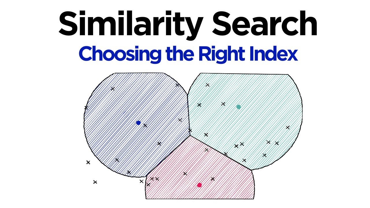
00:22:29.280 | And then that leaves us on to our final index, which is the IVF index. And this is super

00:22:36.400 | popular, and with good reasons. It is very good. So the inverted file index is based

00:22:45.800 | on essentially clustering data points. So we see here, we have all of these different

00:22:51.800 | data points, the little crosses. And then we have these three other points, which are

00:22:57.400 | going to be our cluster centroids. So around each, or based in each of our cluster centroids,

00:23:05.200 | we expand the catchment radius around each of those. And as you can see here, where each

00:23:12.280 | of those circles collides, it creates the edge of what are going to be our almost like

00:23:17.520 | catchment cells. And this is called a Voronoi diagram, or it's a really hard word, Dirichlet

00:23:24.960 | tessellation. I don't know if that's correct, but I think it sounds pretty cool. So I thought

00:23:30.680 | I'd throw that in there. So we create these cells. In each one of those cells, any data

00:23:37.640 | point within those cells will be allocated to that given centroid. And then when you

00:23:44.000 | search within a specific cell, you pass your XQ value in there. And that will be compared,

00:23:52.120 | the XQ value will be compared to every single cluster centroid, but not the other values

00:23:57.640 | within that cluster or the other clusters, only the cluster centroids. And then from

00:24:03.240 | that, you find out which centroid is the closest to your query vector. And then what we do

00:24:10.000 | is we restrict our search scope to only the data points within that cluster or that cell.

00:24:19.400 | And then we calculate the nearest vector. So at this point, we have all the vectors

00:24:25.400 | only within that cell, and we compare all of those to our query vector. Now, there is

00:24:30.280 | one problem with this, which is called the edge problem. Now, we're just showing this

00:24:34.440 | in two-dimensional space. Obviously, in reality, for example, the dataset we're using, we have

00:24:40.280 | 128 dimensions. So dimensionality, the edge problem's kind of complicated when you think

00:24:45.960 | about it in the hundreds of dimensions. But what this is, is say with our query, we find

00:24:54.320 | our query vector is right on the edge of one of the cells. And if we set our nprobe value,

00:25:00.920 | so I mentioned nprobe here, that's how many cells we search. If that is set to one, it

00:25:06.920 | means that we're going to restrict our search to only that cell, even though if you look

00:25:12.000 | at this, we have two, or we have, I'm trying to think. So this one for sure is closer to

00:25:19.640 | our query vector than any of the magenta data points, and possibly also this one and this

00:25:26.560 | one, and maybe even this one. But we're not going to consider any of those because we're

00:25:32.960 | restricting our search only to this cell. So we're only going to look at these data

00:25:41.840 | points and also these over here. So that's the edge problem, but we can get around that

00:25:50.960 | by not just searching one cell, but by searching quite a few. So in this case, our nprobe value

00:25:58.640 | is eight, and that means we're going to search eight of the nearest centroids or centroid

00:26:04.000 | cells. And that's how IVF will work. Let's go ahead and implement that in code. So first

00:26:13.160 | thing we need to do is set our nlist value, which is the number of centroids that we will

00:26:18.100 | have within our data. And then this time, so this is a little bit different, we need

00:26:25.440 | to set the final vector search that we're going to do. So this is split into two different

00:26:32.520 | operations. So we're searching based on clusters, and then we're actually comparing the full

00:26:39.160 | vectors within the selected clusters. So we need to define how we're going to do that

00:26:43.800 | final search between our full vectors and our query vector. So what we do is write FICE.

00:26:52.320 | So we do index flat. We're going to index flat IP. You can use L2 as well. We set our

00:26:57.560 | dimensionality. So we're just initializing a flat index there. And then what we're going

00:27:02.080 | to do is feed that into our IVF index. So our IVF index is FICE, index IVF, and flat,

00:27:11.280 | because we're using the flat indexes, the flat vectors there. We need to pass our quantizer.

00:27:17.520 | So this step here, the other step to the search process, the dimensionality, and also our

00:27:25.840 | nlist value. So how many cells or clusters we're going to have in there. And with this,

00:27:32.040 | because we're clustering data, we need to do something else. So let me show you. So

00:27:38.120 | if we write index.is_trained, we get this false. If we wrote off any of our other indexes,

00:27:45.000 | this would have been true, because they don't need to be trained, because we're not doing

00:27:48.280 | clustering or any other form of training or optimization there. So what we need to do

00:27:54.280 | is we need to train our index before we use it. So we write index_train, and we just pass

00:28:00.200 | all of our vectors into that. It's very quick, so it's not really an issue. And then we do

00:28:08.880 | index add, pass our data. And then what we do, one thing I want to show you, we have

00:28:19.280 | our nprobe value. We'll search with one for now. So we'll search one cell. And to search,

00:28:28.080 | we write di, as we have every other time, search, xq, k. So it's super fast, 3.32 milliseconds.

00:28:40.020 | I think that's maybe the fastest, other than our bad-performing or low-quality HNSUbU index.

00:28:51.300 | So let's see how that's performed. So we write np.in_on_d, baseline. Hi. You see, it's not

00:29:05.220 | too bad, to be fair, like 50/50 almost. So that's actually pretty good. But what we can

00:29:12.820 | do if we want it to be even better is we increase the nprobe value. So let's go up to four.

00:29:19.900 | So that's increased the wartime quite a bit. So from like 3 to 125, which is now super

00:29:25.580 | slow, actually. But now we're getting perfect results. We can maybe decrease that to two.

00:29:32.180 | So now it's faster. That could have been a one-off sometimes. Occasionally, you get a

00:29:35.980 | really slow search. It just happens sometimes. So we set nprobe to two, super fast and super

00:29:46.460 | accurate. So that's a very good index as well. So these are the stats I got in terms of recall

00:29:55.460 | and search time in milliseconds for different nprobe values and different endless values.

00:30:00.880 | So again, it's just about balancing it again. Index size, the only thing that affects your

00:30:08.140 | index size here is obviously the size of your data and the endless value. But you can increase

00:30:12.540 | the endless value loads and the index size hardly increases. So this is like increasing

00:30:17.940 | by 100 kilobytes per double of the endless value. So it's like nothing.

00:30:27.140 | So that's it for this video. And we covered quite a lot. So I'm going to leave it there.

00:30:34.980 | But I think all these indexes are super useful and quite interesting. And figuring out, just

00:30:41.460 | playing around with them. Like you've seen, I've done loads with these graphs, just seeing

00:30:47.540 | what is faster, what is slower, where the good quality is. And just playing around the

00:30:52.260 | parameters and seeing what you can get out of it is super useful for actually understanding

00:30:58.460 | these.

00:31:00.060 | Now what I do want to do going forward is actually explore each one of these indexes

00:31:05.980 | in more depth. Because we've only covered them at a very, very high level at the moment.

00:31:12.940 | So in future videos, articles, we're going to go into more depth and explore them a lot

00:31:20.460 | more. So that will be pretty interesting, I think.

00:31:24.020 | So that's it for this video. Thank you very much for watching. And I'll see you in the

00:31:30.380 | next one. Bye.

00:31:31.260 | [BLANK_AUDIO]

Choosing Indexes for Similarity Search (Faiss in Python)

Chapters