Stanford CS25: V4 I Jason Wei & Hyung Won Chung of OpenAI

00:00:00.000 | So again, I'm very happy to have Jason here.

00:00:07.200 | So he's an AI researcher based in San Francisco,

00:00:09.980 | currently working at OpenAI.

00:00:11.560 | He was previously a research scientist at Google Brain,

00:00:14.380 | where he popularized key ideas in LLMs,

00:00:17.260 | such as chain of thought prompting,

00:00:18.960 | instruction tuning, as well as emergent phenomena.

00:00:21.900 | He's also a good friend of mine,

00:00:23.380 | and he's been here before to give some talks.

00:00:25.320 | So we're very happy to have you back, Jason, and take it away.

00:00:28.980 | Great.

00:00:30.480 | [APPLAUSE]

00:00:33.940 | Yeah.

00:00:34.440 | Thanks for the intro.

00:00:37.020 | So a bit about the structure.

00:00:38.660 | So I'll talk for around 30 minutes,

00:00:40.240 | and then I'll take a few questions.

00:00:41.980 | And then Hyungwon will talk for 30 minutes,

00:00:44.060 | and then we'll both take questions at the end.

00:00:46.020 | Great.

00:00:49.440 | So I want to talk about a few very basic things.

00:00:55.300 | And I think the fundamental question that I hope to get at

00:00:59.780 | is, why do language models work so well?

00:01:09.560 | And one thing that I'd encourage everyone

00:01:14.780 | to do that I found to be extremely helpful in trying

00:01:17.020 | to answer this question is to use a tool, which

00:01:21.780 | is manually inspect data.

00:01:27.260 | And I'll give a short anecdote.

00:01:31.580 | I've been doing this for a long time.

00:01:33.900 | So in 2019, I was trying to build one of the first lung

00:01:38.380 | cancer classifiers.

00:01:39.260 | So there'd be an image, and you have to say, OK,

00:01:41.220 | what type of lung cancer is this?

00:01:43.780 | And my first thing was, OK, if I want

00:01:47.140 | to train a neural network to do this,

00:01:49.520 | I should be able to at least do the task.

00:01:51.220 | So I went to my advisor, and I said,

00:01:53.340 | oh, I want to learn to do this task first.

00:01:55.300 | And he said, Jason, you need a medical degree

00:01:58.300 | and three years of pathology experience

00:02:00.300 | to even do this task.

00:02:01.940 | And I found that a bit discouraging,

00:02:03.740 | but I went and did it anyways.

00:02:05.680 | So I basically looked at the specific type of lung cancer

00:02:09.100 | that I was working on.

00:02:10.660 | And I'd read all the papers on how

00:02:12.340 | to classify different types.

00:02:13.940 | And I went to pathologists, and I said, OK,

00:02:16.060 | try to classify these.

00:02:17.060 | What did I do wrong?

00:02:17.860 | And then, what do you think of that?

00:02:20.140 | And in the end, I learned how to do this task

00:02:22.740 | of classifying lung cancer.

00:02:25.340 | And the result of this was I gained intuitions

00:02:28.340 | about the task that led to many papers.

00:02:32.620 | OK, so first, I will do a quick review of language models.

00:02:38.820 | So the way language models are trained

00:02:41.180 | are with the next word prediction task.

00:02:44.760 | So let's say you have a sentence--

00:02:51.280 | Dartmouth students like to.

00:02:55.640 | And the goal of next word prediction

00:02:57.520 | is you have some words that come before,

00:02:59.440 | and then you want to predict the next word.

00:03:02.080 | And what the language model does is

00:03:05.880 | it outputs a probability for every single word

00:03:08.800 | in the vocabulary.

00:03:10.000 | So vocabulary would be A, aardvark, drink, study,

00:03:21.200 | and then all the way to zucchini.

00:03:24.920 | And then the language model is going

00:03:26.680 | to put a probability over every single word here.

00:03:29.360 | So the probability of A being the next word

00:03:32.160 | is something really small.

00:03:34.680 | Aardvark is something really small.

00:03:37.600 | And then maybe drink is like, say, 0.6.

00:03:40.680 | Study is like 0.3.

00:03:43.800 | Zucchini is, again, really small.

00:03:45.520 | And then the way that you train the language model is you say,

00:03:53.840 | I want--

00:03:54.480 | let's say drink is the correct word here.

00:03:59.040 | I want this number here, 0.6, to be as close as possible to 1.

00:04:03.920 | So your loss is basically, how close

00:04:07.800 | is the probability of the actual next word?

00:04:11.680 | And you want this loss to be as low as possible.

00:04:14.040 | OK, so the first intuition that I would encourage everyone

00:04:27.800 | to use is next word prediction is massively

00:04:45.640 | multi-task learning.

00:04:53.000 | And what I mean by this is the following.

00:04:55.080 | I'll give a few examples.

00:04:56.160 | So when you train a language model on a large enough

00:05:04.880 | database, a large enough data set,

00:05:07.960 | on this task of next word prediction,

00:05:10.560 | you have a lot of sentences that you can learn from.

00:05:12.800 | So for example, there might be some sentence,

00:05:15.800 | in my free time, I like to.

00:05:17.680 | And the language model has to learn

00:05:19.440 | that code should be higher probability than the word

00:05:21.600 | banana.

00:05:22.560 | So learn some grammar.

00:05:25.520 | It'll learn lexical semantics.

00:05:27.160 | So somewhere in your data set, there might be a sentence,

00:05:31.560 | I went to the store to buy papaya, dragon fruit,

00:05:34.080 | and durian.

00:05:35.440 | And the language model should know

00:05:36.900 | that the probability of durian should be higher than squirrel.

00:05:41.240 | The language model will learn world knowledge.

00:05:43.420 | So there will be some sentence on the internet that says,

00:05:45.760 | you know, the capital of Azerbaijan is--

00:05:48.160 | and then the language model should learn that it should be

00:05:50.620 | Baku instead of London.

00:05:53.760 | You can learn traditional NLP tasks, like sentiment analysis.

00:05:56.640 | So there'll be some sentence, you know,

00:05:58.440 | I was engaged on the edge of my seat the whole time.

00:06:00.720 | The movie was.

00:06:01.960 | And the language model looks like, OK,

00:06:03.560 | these are the prior next words.

00:06:05.480 | The next word should probably be good and not bad.

00:06:10.200 | And then finally, another example is translation.

00:06:14.240 | So here, you might see some sentence,

00:06:16.660 | the word for pretty in Spanish is.

00:06:19.240 | And then the language model should

00:06:21.120 | weigh Bonita more than Ola.

00:06:24.960 | Spatial reasoning.

00:06:26.120 | So you might even have some sentence like,

00:06:28.200 | Iroh went to the kitchen to make some tea.

00:06:30.360 | Standing next to Iroh, Zuko pondered his destiny.

00:06:33.560 | Zuko left the.

00:06:34.880 | And then kitchen should be higher probability than store.

00:06:39.000 | And then finally, even some math questions.

00:06:41.160 | So you might have, like, some arithmetic exam answer

00:06:44.720 | key somewhere on the internet.

00:06:46.480 | And then the language model looks at this and says,

00:06:48.600 | OK, the next word should probably be 15 and not 11.

00:06:53.360 | And you can have, like, basically millions

00:06:55.120 | of tasks like this when you have a huge data set.

00:06:58.720 | And you can think of this as basically

00:07:00.800 | extreme multitask learning.

00:07:03.840 | And these are sort of like very clean examples of tasks.

00:07:08.160 | But I'll give an example of how arbitrary

00:07:16.360 | some of these tasks can be.

00:07:17.600 | So here's a sentence from Wikipedia.

00:07:26.800 | Biden married Amelia.

00:07:34.920 | And then now, pretend you're the language model.

00:07:37.880 | And you could say, like, OK, what's the next word here?

00:07:41.560 | And the next word here is Hunter.

00:07:44.160 | So it's Biden's first wife.

00:07:46.360 | And so, like, OK, what's the language model learning

00:07:48.640 | from predicting this word?

00:07:50.160 | I guess, like, world knowledge.

00:07:52.200 | And then what's the next word after this?

00:07:58.720 | Turns out the next word is a comma.

00:08:00.760 | So here, the model is learning, like, basically

00:08:03.360 | comma prediction.

00:08:06.800 | And then what's the next word after that?

00:08:09.840 | I think it's kind of hard to know, but the answer is A.

00:08:13.320 | And I guess this is, like, maybe grammar,

00:08:15.720 | but, like, somewhat arbitrary.

00:08:17.480 | And then what's the next word after that?

00:08:23.480 | Turns out it's student.

00:08:24.680 | And this, I would say, I don't know what task this is.

00:08:31.040 | This is, like, you know, it could have been woman.

00:08:35.160 | It could have been something else.

00:08:37.160 | So this is, like, a pretty arbitrary task.

00:08:40.040 | And the point that I'm trying to make here

00:08:41.960 | is that the next word prediction task is really challenging.

00:08:45.520 | So, like, if you do this over the entire database,

00:08:47.680 | you're going to learn a lot of tasks.

00:08:51.240 | OK.

00:08:51.740 | The next intuition I want to talk about

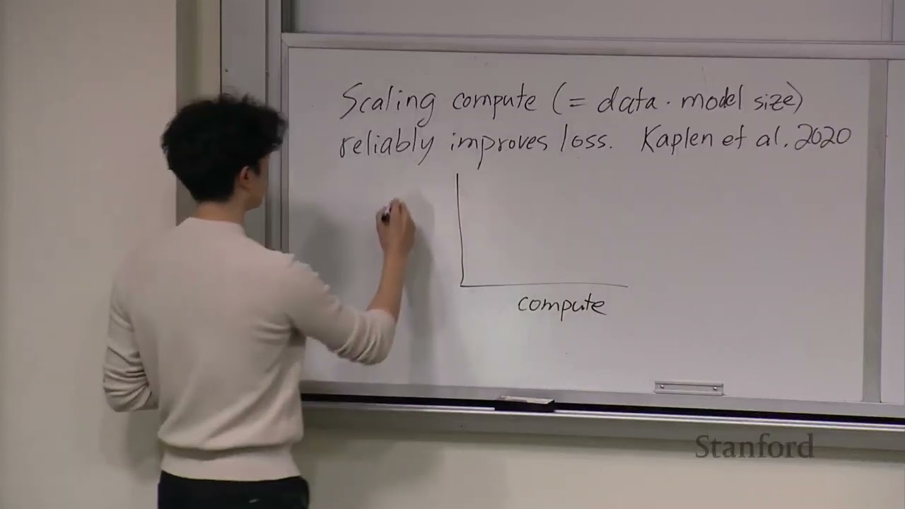
00:09:01.520 | is scaling, which is, by the way, let's say scaling compute.

00:09:15.960 | And by the way, compute is equal to how much data you have

00:09:19.720 | times the size of language model.

00:09:21.400 | Reliably improves loss.

00:09:29.320 | [WRITING ON BOARD]

00:09:32.240 | And this idea was basically pioneered

00:09:40.640 | by Kaplan et al in 2020.

00:09:47.200 | I would encourage you guys to read the paper.

00:09:49.600 | And what this basically says is you can have a plot here,

00:09:54.200 | and we'll see many plots like this,

00:09:56.320 | where the x-axis is compute and the y-axis is loss.

00:10:05.920 | And what this intuition says is you can train one language

00:10:10.120 | model, you'll have that loss.

00:10:11.760 | And obviously, you want loss to be lower.

00:10:13.960 | So you can train the next one, you'll have that loss.

00:10:16.480 | If you train the one after that, you'll have that loss.

00:10:19.120 | Then if you train the one after that, you'll have that loss.

00:10:22.680 | And you can basically predict the loss of a language model

00:10:26.300 | based on how much compute you're going to use to train it.

00:10:30.040 | And the reason why this is called a law

00:10:32.560 | is that in this paper, they showed that the x-axis here

00:10:36.640 | is actually seven orders of magnitude.

00:10:39.320 | So basically, it would be surprising if the trend broke

00:10:42.600 | if you continued.

00:10:44.800 | And the important thing about this

00:10:47.200 | is that the line does not go like that.

00:10:50.200 | Because if it went like that, then it would saturate.

00:10:55.120 | And then putting more compute or training a larger language

00:10:57.580 | model wouldn't actually lead to lower loss.

00:11:00.440 | So I think a question that we don't have a good answer

00:11:18.660 | to as a field, but I'll give you a hand-wavy answer,

00:11:22.980 | is why does scaling up the size of your language model

00:11:26.900 | improve the loss?

00:11:28.980 | And I'll give two basically hand-wavy answers.

00:11:31.300 | So here's a small lm, and here's large lm.

00:11:39.340 | So one thing that's important is how good is your language model

00:11:43.100 | at memorizing facts?

00:11:44.580 | And imagine you're a small language model,

00:11:50.780 | and you see a bunch of facts on the internet.

00:11:53.660 | You have to be pretty choosy in which facts you memorize.

00:11:57.220 | Because if you don't have that many parameters,

00:11:59.140 | you're like, oh, I can only memorize a million facts.

00:12:01.740 | Is this one of the facts I want to memorize

00:12:03.580 | to get the lowest loss?

00:12:05.020 | And so you have to be very selective.

00:12:07.700 | Whereas if you're a large language model,

00:12:12.980 | you can memorize a lot of tail knowledge.

00:12:15.580 | And so basically, every fact you see,

00:12:17.180 | you don't have to say, oh, is this

00:12:18.420 | something I want to memorize?

00:12:19.700 | You can just memorize it.

00:12:22.020 | And then the other hand-wavy answer I'll give

00:12:25.460 | is small language models tend to learn first-order heuristics.

00:12:31.980 | So if you're a small language model,

00:12:35.260 | you're already struggling to get the grammar correct.

00:12:37.980 | You're not going to do your best to try to get the math

00:12:40.300 | problem exactly correct.

00:12:42.420 | Whereas if you're a large language model,

00:12:46.860 | you have a lot of parameters in your forward pass.

00:12:50.100 | And you can try to do really complicated things

00:12:52.300 | to get the next token correct and to get

00:12:54.820 | the loss as low as possible.

00:12:56.060 | So the third intuition I'll talk about

00:13:11.060 | is while overall loss improves smoothly,

00:13:26.660 | individual tasks can improve suddenly.

00:13:42.060 | And here's what I mean by this.

00:13:44.020 | So you can write your overall loss.

00:13:47.540 | By this, I mean if you take some corpus of data

00:13:53.580 | and you compute the overall loss on every word in that data set.

00:13:58.140 | The overall loss, because we know that next word prediction

00:14:01.900 | is massively multitask learning, you

00:14:04.060 | can decompose this overall loss into the loss

00:14:06.980 | of every single individual task.

00:14:08.700 | So you have, I don't know, some small number times the loss

00:14:14.660 | of, say, grammar plus some small number times

00:14:21.300 | the loss of sentiment analysis plus some small number

00:14:30.380 | times the loss of world knowledge plus--

00:14:37.180 | and then all the way to, let's say,

00:14:38.820 | you have something times the loss of math.

00:14:47.500 | And so you can basically write your overall loss

00:14:49.940 | as the weighted sum of the individual tasks

00:14:52.540 | in the data set.

00:14:54.700 | And now the question is, let's say

00:14:56.900 | I improve my loss from 4 to 3.

00:15:01.740 | Do each of these individual tasks

00:15:03.460 | improve at the same rate?

00:15:06.580 | Well, I'd say probably not.

00:15:07.740 | So if you have a good enough language model,

00:15:11.580 | it's already doing basically perfectly

00:15:13.180 | on grammar and sentiment analysis.

00:15:15.380 | So this might not improve.

00:15:19.540 | This might be saturated.

00:15:21.100 | And maybe the loss on math is not saturated.

00:15:29.260 | It's not that good at math yet.

00:15:30.840 | So this could improve suddenly.

00:15:32.140 | And I'll redraw the diagram to show this.

00:15:47.140 | So again, compute here and loss here.

00:15:55.580 | And your overall loss is like this.

00:15:57.860 | What I'm saying is there might be

00:16:05.940 | some part of that overall loss that scales like this.

00:16:09.420 | So this is, say, grammar.

00:16:13.220 | So for example, you could say, if GPT 3.5 is there

00:16:18.100 | and GPT 4 is there, you haven't actually

00:16:20.540 | improved the grammar that much.

00:16:23.060 | On the other hand, you might have something

00:16:25.780 | like this for, say, doing math or harder tasks,

00:16:30.380 | where the difference between GPT 3.5 and GPT 4

00:16:34.300 | will be much larger.

00:16:37.420 | And it turns out you can look at a big set of tasks, which

00:16:48.920 | I did, and you can look at what's

00:16:51.100 | the shape of these scaling curves.

00:16:54.340 | So I looked at 202 tasks.

00:16:58.900 | There's this corpus called Big Bench, which has 200 tasks.

00:17:02.060 | I looked at all of them.

00:17:03.860 | And here is the distribution.

00:17:06.300 | So you have-- this was 29% of tasks that were smooth.

00:17:17.380 | So if I draw the scaling plot, compute is on the x-axis.

00:17:23.380 | And then here we have accuracy instead of loss.

00:17:25.620 | So higher is better.

00:17:27.700 | Then you have something like this.

00:17:31.140 | I believe this was 22% will be flat.

00:17:36.860 | So if you have your scaling curve, it'll just all be 0.

00:17:39.740 | The task was too hard.

00:17:42.620 | 2% will be something called inverse scaling.

00:17:46.300 | I'll talk about this in a sec.

00:17:49.140 | But what that means is the accuracy actually

00:17:52.580 | gets worse as you increase the size of the language model.

00:17:57.180 | And then I think this was 13% will be not correlated.

00:18:03.340 | So you have something like that.

00:18:09.300 | I don't know.

00:18:10.540 | And then finally, a pretty big portion, 33%,

00:18:16.380 | will be emergent abilities.

00:18:21.380 | And what I mean by that is if you plot your compute

00:18:28.140 | and accuracy, for a certain point, up to a certain point,

00:18:35.100 | your accuracy will be 0.

00:18:37.460 | And then the accuracy suddenly starts to improve.

00:18:42.020 | And so you can define an emergent ability basically

00:18:45.820 | as, for small models, the performance is 0.

00:18:52.700 | So it's not present in this model.

00:18:54.700 | And then for large models, you have much better

00:19:03.060 | than random performance.

00:19:04.940 | And the interesting thing about this

00:19:06.660 | is, let's say you had only trained the small language

00:19:09.520 | models up to that point.

00:19:10.880 | You would have predicted that it would have been impossible

00:19:13.460 | for the language model to ever perform the task.

00:19:16.580 | But actually, when you train the larger model,

00:19:18.540 | the language model does learn to perform the task.

00:19:20.900 | So in a sense, it's pretty unpredictable.

00:19:23.980 | I'll talk about one final thing, which

00:19:39.140 | is something called inverse scaling slash u-shaped scaling.

00:19:45.660 | OK, so I'll give a tricky prompt to illustrate this.

00:19:52.580 | So the tricky prompt is this.

00:19:55.620 | Repeat after me, all that glisters is not glib.

00:20:12.860 | All that glisters is not.

00:20:23.020 | And this is the prompt I give to the language model.

00:20:26.220 | And the goal is to predict this next word.

00:20:29.100 | And obviously, the correct answer

00:20:31.580 | is glib, because you asked to repeat after me.

00:20:37.220 | And what you see is, let's say you

00:20:40.460 | have a extra small language model, a small language model,

00:20:45.580 | and a large language model.

00:20:48.100 | The performance for the extra small language model

00:20:51.060 | will be, say, here's 100%.

00:20:55.580 | The small language model is actually worse at this task.

00:20:59.340 | So it's something like something here.

00:21:01.260 | And then the large language model, again,

00:21:03.980 | learns to do this task.

00:21:06.540 | So how do we basically explain a behavior

00:21:09.140 | like this for a prompt like this?

00:21:10.940 | [WRITING]

00:21:14.380 | And the answer is, you can decompose this prompt

00:21:26.220 | into three subtasks that are basically being done.

00:21:30.620 | So the first subtask is, can you repeat some text?

00:21:33.900 | Right?

00:21:36.340 | And if you draw the plot here, again,

00:21:39.340 | extra small, small, large, and then here is 100.

00:21:44.540 | This is a super easy task.

00:21:46.420 | And so all the language models have

00:21:51.460 | perfect performance on that.

00:21:53.580 | That's one hidden task.

00:21:55.180 | The other task is, can you fix a quote?

00:22:02.020 | So the quote is supposed to be, all that glisters is not gold.

00:22:05.860 | And so you can then plot, again, extra small, small, large.

00:22:12.380 | What's the ability to fix that quote?

00:22:14.740 | Well, the small language model doesn't know the quote.

00:22:17.300 | So it's going to get 0.

00:22:19.860 | And then the extra small doesn't know the quote,

00:22:22.020 | so it's going to get 0.

00:22:23.540 | The small will be able to do it.

00:22:26.020 | And the large can obviously do it.

00:22:28.300 | So that's what the scaling curve looks like.

00:22:31.780 | And then finally, you have the quote--

00:22:37.060 | you have the task, follow an instruction.

00:22:40.420 | And obviously, this is the instruction here.

00:22:47.060 | And you could say, OK, what's the performance

00:22:49.860 | of these models on this task?

00:22:52.220 | And the small model can't do it, or the extra small model

00:22:59.580 | can't do it.

00:23:00.620 | Small model also can't do it.

00:23:02.460 | But the large model can do it.

00:23:04.740 | So you get a curve like this.

00:23:07.540 | And then why does this explain this behavior here?

00:23:11.260 | Well, the extra small model, it can repeat.

00:23:16.660 | It can't fix the quote.

00:23:18.180 | And it can't follow the instruction.

00:23:19.940 | So it actually gets it correct.

00:23:21.180 | It says glib.

00:23:23.500 | It says glib.

00:23:26.380 | The small model can repeat.

00:23:30.700 | It can fix the quote.

00:23:32.020 | But it doesn't follow the instruction.

00:23:33.740 | So it decides to fix the quote.

00:23:35.060 | And then the large model, it can do all three.

00:23:42.420 | It can follow the instruction.

00:23:43.980 | So it just repeats.

00:23:44.740 | And so that's how, if you look at the individual subtasks,

00:23:52.700 | you can explain the behavior of some of these weird scaling

00:23:55.620 | properties.

00:23:56.580 | So I will conclude with one general takeaway, which

00:24:11.260 | is applicable if you do research.

00:24:15.460 | And the takeaway is to just plot scaling curves.

00:24:20.660 | ,

00:24:26.060 | And I'll just give a really simple example.

00:24:28.380 | So let's say I do something for my research project.

00:24:32.340 | I fine-tune a model on some number of examples.

00:24:37.100 | And I get-- this is my thing.

00:24:42.540 | I get some performance there.

00:24:45.540 | And then here's the baseline.

00:24:48.460 | Of not doing whatever my research project is.

00:24:53.700 | And there's the performance.

00:24:56.660 | The reason you want to plot a scaling curve for this

00:24:59.180 | is, let's say you take half the data.

00:25:02.740 | And you find out that the performance is actually here.

00:25:06.660 | So your curve looks like this.

00:25:09.980 | What this would tell you is you didn't

00:25:11.940 | have to collect all the data to do your thing.

00:25:14.180 | And if you collect more, you probably

00:25:16.420 | won't see an improvement in performance.

00:25:19.900 | Another scenario would be if you plotted that point

00:25:23.860 | and it was there, then your curve will look like this.

00:25:28.100 | And potentially, if you kept doing

00:25:30.940 | more of whatever your research project is,

00:25:33.620 | you'd see an improvement in performance.

00:25:37.020 | And then finally, maybe your point is there.

00:25:40.740 | So your curve looks like this.

00:25:43.380 | And in this case, you would expect

00:25:45.340 | to see an even larger jump in performance

00:25:48.340 | after you continue doing your thing.

00:25:51.460 | So yeah, I'll end my talk here.

00:25:54.660 | And I'm happy to take a few questions beforehand

00:25:57.020 | while I talk.

00:25:57.520 | Yeah.

00:26:01.900 | Go ahead.

00:26:02.900 | [INAUDIBLE]

00:26:10.380 | Data that has an operational source,

00:26:12.300 | do you break the data [INAUDIBLE]

00:26:13.860 | based on the source?

00:26:15.620 | Repeat the question.

00:26:16.580 | Oh.

00:26:17.080 | Oh, yeah.

00:26:17.580 | Yeah, thanks.

00:26:18.380 | Good question.

00:26:19.620 | So the question is, during pre-training,

00:26:23.900 | how do you differentiate between good data and bad data?

00:26:27.820 | The question is-- or the answer is, you don't really.

00:26:31.380 | But you should by only training on good data.

00:26:33.540 | So maybe you should look at your data source

00:26:37.620 | and filter out some data if it's not from a reliable data source.

00:26:40.860 | Do you want to give us maybe the intuition

00:26:46.180 | behind the intuition for one or two of the examples,

00:26:48.780 | like emergent, or why tail knowledge starts to develop?

00:26:54.460 | What's behind that?

00:26:55.980 | What do you mean, intuition behind intuition?

00:26:58.520 | Intuitively, these concepts that you're seeing in the graphs.

00:27:01.460 | And from your experience and expertise,

00:27:04.060 | what in the model itself is really

00:27:07.060 | causing that emergent behavior?

00:27:08.700 | What do you mean, in the model itself?

00:27:14.660 | Is it more depth, more nodes, more--

00:27:19.260 | Oh, I see.

00:27:19.780 | --attention, in an intuitive sense, not in a--

00:27:24.060 | Oh, yeah, OK, yeah.

00:27:24.860 | So the question is, what in the model

00:27:26.620 | makes the language model better at memorizing tail knowledge

00:27:30.300 | or at doing math problems?

00:27:35.860 | Yeah, I think it's definitely related to the size

00:27:37.940 | of the language model.

00:27:38.940 | So yeah, if you have more layers,

00:27:41.620 | you could encode probably a more complex function within that.

00:27:46.220 | And then I guess if you have more breadth,

00:27:49.780 | you could probably encode more facts about the world.

00:27:54.140 | And then if you want to repeat a fact or retrieve something,

00:27:57.340 | it'd probably be easier.

00:27:59.340 | We'll get one more in person, and then I'll

00:28:01.340 | move this more slowly.

00:28:04.340 | Hi.

00:28:05.100 | So when you were studying the 200-ish problems

00:28:07.980 | in the big bench, you noticed that 22% were flat.

00:28:11.580 | But there's a possibility that if you were to increase

00:28:13.820 | the compute even further, those might

00:28:15.500 | have turned out to be emergent.

00:28:16.780 | So my question to you is that when

00:28:18.300 | you were looking at the 33% that turned out to be emergent,

00:28:21.300 | did you notice anything about the loss in the flat portion

00:28:24.060 | that suggested that it would eventually become emergent?

00:28:27.460 | Oh, yeah.

00:28:29.140 | I didn't notice anything.

00:28:31.180 | Oh, sorry.

00:28:31.700 | Let me repeat the question.

00:28:32.980 | The question is, when I looked at all the emergent tasks,

00:28:36.980 | was there anything that I noticed before the emergence

00:28:40.140 | point in the loss that would have hinted that it

00:28:43.420 | would become emergent later?

00:28:45.420 | To me, it's kind of tough.

00:28:46.460 | We have a few plots of this.

00:28:48.380 | You can look at the loss, and it kind of gets better.

00:28:51.480 | And then suddenly, it spikes, and there's

00:28:53.180 | no way to predict it.

00:28:54.100 | But also, you don't have perfect data,

00:28:56.340 | because you might not have all the intermediate points

00:28:58.660 | for a given model size.

00:29:00.740 | Yeah.

00:29:01.240 | Great question.

00:29:01.900 | Yeah, we can move to [INAUDIBLE]

00:29:08.260 | We have a few online questions.

00:29:10.140 | Oh, OK.

00:29:10.660 | Yeah.

00:29:11.160 | We just have a few questions from people

00:29:12.980 | who are joining on Zoom.

00:29:15.020 | The first one is, what do you think

00:29:16.580 | are the biggest bottlenecks for current large language models?

00:29:19.380 | Is it the quality of data, the amount of compute,

00:29:21.860 | or something else?

00:29:24.940 | Yeah, great question.

00:29:25.900 | I guess if you go back to the scaling loss paradigm, what

00:29:32.860 | it says is that if you increase the size of the data

00:29:36.400 | and the size of the model, then you'd

00:29:38.500 | expect to get a lot better performance.

00:29:40.540 | And I think we'll probably try to keep increasing those things.

00:29:43.780 | Gotcha.

00:29:44.380 | And then the last one, what are your thoughts on the paper,

00:29:48.020 | if you've read it?

00:29:49.220 | Are emergent abilities of large language models a mirage?

00:29:53.260 | Oh, yeah.

00:29:53.740 | I always get this question.

00:29:55.640 | I guess I would encourage you to read the paper

00:29:58.640 | and decide for yourself.

00:29:59.860 | But I guess what the paper says is if you change the metric a

00:30:05.660 | bit, it looks different.

00:30:07.380 | But I would say, at the end of the day,

00:30:10.700 | I think the language model abilities are real.

00:30:12.660 | And if you think--

00:30:14.300 | I guess I don't think that's a mirage.

00:30:16.340 | So, yeah.

00:30:19.580 | Yeah.

00:30:25.340 | All right, so thanks, Jason, for the very insightful talk.

00:30:28.580 | And now we'll have Hyung Won give a talk.

00:30:31.500 | So he's currently a research scientist

00:30:34.420 | on the OpenAI Chat GPT team.

00:30:36.700 | He has worked on various aspects of large language models,

00:30:40.780 | things like pre-training, instruction fine-tuning,

00:30:43.380 | reinforcement learning with human feedback, reasoning,

00:30:47.060 | and so forth.

00:30:48.060 | And some of his notable works include the scaling FLAN

00:30:50.820 | papers, such as FLAN T5, as well as FLAN POM, and T5X,

00:30:55.220 | the training framework used to train the POM language model.

00:30:58.660 | And before OpenAI, he was at Google Brain,

00:31:01.220 | and he received his PhD from MIT.

00:31:04.700 | So give a hand for Hyung Won.

00:31:06.220 | All right, my name is Hyung Won, and really happy

00:31:21.180 | to be here today.

00:31:22.300 | And this week, I was thinking about--

00:31:24.940 | by the way, is my mic working fine?

00:31:27.660 | Yeah, yeah.

00:31:28.580 | So this week, I thought about, OK,

00:31:30.500 | I'm giving a lecture on transformers at Stanford.

00:31:34.020 | What should I talk about?

00:31:35.380 | And I thought, OK, some of you in this room and in Zoom

00:31:39.860 | will actually go shape the future of AI.

00:31:42.120 | So maybe I should talk about that.

00:31:43.540 | It's a really important goal and ambitious,

00:31:45.460 | and we really have to get it right.

00:31:47.220 | So that could be a good topic to think about.

00:31:50.140 | And when we talk about something into the future,

00:31:53.620 | the best place to get an advice is to look into the history.

00:31:57.860 | And in particular, look at the early history of transformer

00:32:01.960 | and try to learn many lessons from there.

00:32:04.660 | And the goal will be to develop a unified perspective in which

00:32:10.380 | we can look into many seemingly disjoint events.

00:32:13.860 | And from that, we can probably hope

00:32:17.340 | to project into the future what might be coming.

00:32:20.260 | And so that will be the goal of this lecture.

00:32:24.420 | And we'll look at some of the architectures

00:32:26.260 | of the transformers.

00:32:27.460 | So let's get started.

00:32:30.020 | Everyone I see is saying AI is so advancing so fast that

00:32:34.860 | it's so hard to keep up.

00:32:36.420 | And it doesn't matter if you have years of experience.

00:32:39.340 | There's so many things that are coming out every week

00:32:41.780 | that it's just hard to keep up.

00:32:43.420 | And I do see many people spend a lot of time and energy

00:32:46.940 | catching up with the latest developments, the cutting

00:32:50.340 | edge and the newest thing.

00:32:52.580 | And then not enough attention goes into all things

00:32:54.980 | because they become deprecated and no longer relevant.

00:33:00.740 | But I think it's important, actually, to look into that.

00:33:03.220 | Because we really need to--

00:33:05.460 | when things are moving so fast beyond our ability

00:33:08.060 | to catch up, what we need to do is study the change itself.

00:33:11.460 | And that means we can look back at the previous things

00:33:14.660 | and then look at the current thing

00:33:16.660 | and try to map how we got here and from which we can look

00:33:20.020 | into where we are heading towards.

00:33:23.060 | So what does it mean to study the change itself?

00:33:28.140 | First, we need to identify the dominant driving

00:33:31.740 | forces behind the change.

00:33:33.540 | So here, dominant is an important word

00:33:35.900 | because typically, a change has many, many driving forces.

00:33:39.700 | And we only care about the dominant one

00:33:41.420 | because we're not trying to get really accurate.

00:33:43.460 | We just want to have the sense of directionality.

00:33:46.220 | Second, we need to understand the driving force really well.

00:33:49.220 | And then after that, we can predict the future trajectory

00:33:52.100 | by rolling out the driving force and so on.

00:33:55.620 | And you heard it right.

00:33:56.620 | I mentioned about predicting the future.

00:33:58.620 | This is a computer science class, not

00:34:00.140 | like an astrology or something.

00:34:01.780 | But we do--

00:34:02.820 | I think it's actually not that impossible to predict

00:34:06.660 | some future trajectory of a very narrow scientific domain.

00:34:10.380 | And that endeavor is really useful to do

00:34:14.380 | because let's say you do all these

00:34:17.540 | and then make your prediction accuracy from 1% to 10%.

00:34:21.620 | And then you'll make, say, 100 predictions.

00:34:23.860 | 10 of them will be correct.

00:34:25.500 | Say, one of them will be really, really correct,

00:34:27.860 | meaning it will have an outside impact that

00:34:30.100 | outweighs everything.

00:34:31.580 | And I think that is kind of how many--

00:34:35.060 | I've seen a very general thing in life

00:34:37.620 | that you really have to be right a few times.

00:34:40.340 | So if we think about why predicting the future

00:34:47.260 | is difficult, or maybe even think about the extreme case

00:34:50.180 | where we can all do the prediction

00:34:53.100 | with perfect accuracy, almost perfect accuracy.

00:34:55.460 | So here, I'm going to do a very simple experiment

00:34:58.500 | of dropping this pen and follow this same three-step process.

00:35:04.100 | So we're going to identify the dominant driving force.

00:35:07.300 | First of all, what are the driving forces acting

00:35:09.340 | on this pen, gravity downwards?

00:35:11.500 | And is that all?

00:35:12.300 | We also have, say, air friction if I drop it.

00:35:17.380 | And that will cause what's called a drag force acting

00:35:20.380 | upwards.

00:35:21.380 | And actually, depending on how I drop this, the orientation,

00:35:25.620 | the aerodynamic interaction will be so complicated

00:35:28.860 | that we don't currently have any analytical way of modeling

00:35:32.100 | that.

00:35:32.700 | We can do it with the CFD, the computational fluid dynamics,

00:35:35.580 | but it will be nontrivial.

00:35:36.820 | So we can neglect that.

00:35:38.780 | This is heavy enough that gravity is probably

00:35:40.700 | the only dominant force.

00:35:41.740 | We simplify the problem.

00:35:44.100 | Second, do we understand this dominant driving force, which

00:35:46.900 | is gravity?

00:35:47.780 | And we do because we have this Newtonian mechanics, which

00:35:50.660 | provides a reasonably good model.

00:35:52.500 | And then with that, we can predict the future trajectory

00:35:55.060 | of this pen.

00:35:56.420 | And if you remember from this dynamics class,

00:35:59.740 | if we have this initial velocity is 0,

00:36:02.420 | I'm not going to put any velocity.

00:36:04.140 | And then let's say position is 0 here.

00:36:06.180 | And then 1/2 gt square will give a precise trajectory

00:36:11.380 | of this pen as I drop this.

00:36:13.500 | So if there is a single driving force that we really

00:36:17.140 | understand, it's actually possible to predict

00:36:19.980 | what's going to happen.

00:36:21.500 | So then why do we really fear about predicting the future

00:36:26.380 | in the most general sense?

00:36:27.900 | And I argue that among many reasons,

00:36:30.660 | the number of driving force, the sheer number

00:36:33.140 | of dominant driving forces acting on the general prediction

00:36:37.100 | is so complicated.

00:36:38.540 | And their interaction creates a complexity

00:36:41.140 | that we cannot predict the most general sense.

00:36:43.580 | So here's my cartoon way of thinking

00:36:45.220 | about the prediction of future.

00:36:47.420 | X-axis, we have a number of dominant driving forces.

00:36:50.020 | Y-axis, we have a prediction difficulty.

00:36:52.180 | So on the left-hand side, we have a dropping a pen.

00:36:54.660 | It's a very simple case.

00:36:56.260 | It's a difficulty.

00:36:57.020 | It's very small.

00:36:57.780 | You just need to learn physics.

00:37:00.540 | And then as you add more stuff, it just becomes impossible.

00:37:05.300 | So how does this fit into the AI research?

00:37:08.180 | And you might think, OK, I see all the time things

00:37:12.340 | are coming in.

00:37:13.060 | We are bombarded by new things.

00:37:15.220 | And some people will come up with a new agent, new modality,

00:37:18.460 | new MML use score, whatever.

00:37:20.100 | We just see so many things.

00:37:22.900 | I'm not even able to catch up with the latest thing.

00:37:25.700 | How can I even hope to predict the future of the AI research?

00:37:29.300 | But I argue that it's actually simpler,

00:37:31.780 | because there is a dominant driving force that

00:37:35.180 | is governing a lot, if not all, of the AI research.

00:37:39.420 | And because of that, I would like

00:37:41.460 | to point out that it's actually closer to the left

00:37:45.180 | than to the right than we actually may perceive.

00:37:49.140 | So what is that driving force?

00:37:52.220 | Oh, maybe before that, I would like

00:37:53.940 | to caveat that when I do this kind of talk,

00:37:58.420 | I would like to not focus too much

00:38:00.540 | on the technical stuff, which you can probably

00:38:02.860 | do better in your own time.

00:38:05.020 | But rather, I want to share how I think.

00:38:07.780 | And for that, I want to share how my opinion is.

00:38:11.860 | And so it will be very strongly opinionated.

00:38:14.580 | And by no means, I'm saying this is correct or not.

00:38:17.780 | Just wanted to share my perspective.

00:38:19.820 | So coming back to this driving force for AI,

00:38:22.180 | what is that dominant driving force?

00:38:24.540 | And here is a plot from Rich Sutton.

00:38:27.260 | And on the y-axis, we have the calculations flopped.

00:38:31.620 | If you pay $100, and how much computing power do you get?

00:38:36.020 | And it's in log scale.

00:38:37.500 | And then x-axis, we have a time of more than 100 years.

00:38:42.260 | So this is actually more than exponential.

00:38:45.100 | And I don't know any trend that is as strong and as

00:38:49.740 | long-lasting as this one.

00:38:51.300 | So whenever I see this kind of thing, I should say, OK,

00:38:55.860 | I should not compete with this.

00:38:57.540 | And better, I should try to leverage as much as possible.

00:39:01.700 | And so what this means is you get 10x more compute

00:39:07.180 | every five years if you spend the same amount of dollar.

00:39:10.460 | And so in other words, you get the cost of compute

00:39:14.660 | is going down exponentially.

00:39:16.260 | And this and associated scaling is really

00:39:19.820 | dominating the AI research.

00:39:22.220 | And that is somewhat hard to take.

00:39:24.180 | But that is, I think, really important to think about.

00:39:27.620 | So coming back to this AI research,

00:39:29.580 | how is this exponentially cheaper

00:39:32.380 | compute drive the AI research?

00:39:35.180 | Let's think about the job of the AI researchers.

00:39:37.580 | It is to teach machines how to think in a very general sense.

00:39:41.260 | And one somewhat unfortunately common approach

00:39:45.220 | is we think about how we teach machine how we think we think.

00:39:50.900 | So meaning we model how we think and then

00:39:55.420 | try to incorporate that into some kind of mathematical model

00:39:58.100 | and teach that.

00:39:59.380 | And now the question is, do we understand

00:40:01.580 | how we think at the very low level?

00:40:03.860 | I don't think we do.

00:40:05.220 | I have no idea what's going on.

00:40:06.940 | So it's fundamentally flawed in the sense

00:40:08.860 | that we try to model something that we have no idea about.

00:40:11.860 | And what happens if we go with this kind of approach

00:40:14.460 | is that it poses a structure that

00:40:16.620 | serves as a shortcut in the short term.

00:40:19.020 | And so you can maybe get a paper or something.

00:40:21.420 | But then it becomes a bottleneck,

00:40:23.780 | because we don't know how this will limit further scaling up.

00:40:29.020 | More fundamentally, what this is doing

00:40:30.900 | is we are limiting the degree of freedom

00:40:33.740 | we are giving to the machines.

00:40:35.620 | And that will backfire at some point.

00:40:37.600 | And this has been going on for decades.

00:40:42.180 | And bitter lesson is, I think, the single most important piece

00:40:46.940 | of writing in AI.

00:40:48.660 | And it says-- this is my wording, by the way--

00:40:51.660 | past 70 years of entire AI research

00:40:54.300 | can be summarized into developing progressively more

00:40:57.980 | general method with weaker modeling assumptions

00:41:01.020 | or inductive biases, and add more data and compute--

00:41:03.660 | in other words, scale up.

00:41:04.860 | And that has been the recipe of entire AI research,

00:41:08.820 | not fancy things.

00:41:10.380 | And if you think about this, the models of 2000

00:41:14.460 | is a lot more difficult than what we use now.

00:41:17.900 | And so it's much easier to get into AI nowadays

00:41:21.100 | from a technical perspective.

00:41:22.900 | So this is, I think, really the key information.

00:41:27.820 | We have this compute cost that's going down exponentially.

00:41:31.000 | And it's getting cheaper faster than we're

00:41:33.340 | becoming a better researcher.

00:41:34.780 | So don't compete with that.

00:41:36.260 | And just try to leverage that as much as possible.

00:41:38.740 | And that is the driving force that I wanted to identify.

00:41:43.500 | And I'm not saying this is the only driving force.

00:41:46.260 | But this is the dominant driving force.

00:41:47.920 | So we can probably neglect the other ones.

00:41:50.100 | So here's a graphical version of that.

00:41:52.020 | X-axis, we have a compute.

00:41:53.380 | Y-axis, we have a performance of some kind.

00:41:55.460 | Let's think about some general intelligence.

00:41:57.780 | And let's look at two different methods, one

00:42:00.800 | with more structure, more modeling assumptions, fancier

00:42:03.580 | math, whatever.

00:42:04.660 | And then the other one is a less structure.

00:42:06.420 | What you see is typically you start with a better performance

00:42:10.740 | when you have a low compute regime.

00:42:13.140 | But it plateaus because of some kind of structure backfiring.

00:42:16.120 | And then with the less structure,

00:42:17.460 | because we give a lot more freedom to the model,

00:42:19.780 | it doesn't work in the beginning.

00:42:21.380 | But then as we add more compute, it starts working.

00:42:23.940 | And then it gets better.

00:42:25.580 | We call this more scalable methods.

00:42:28.460 | So does that mean we should just go

00:42:30.820 | with the least structure, most freedom

00:42:33.540 | to the model possible way from the get-go?

00:42:36.420 | And the answer is obviously no.

00:42:38.180 | Let's think about even less structure case.

00:42:40.220 | This red one here, it will pick up a lot later

00:42:44.620 | and requires a lot more compute.

00:42:46.820 | So it really depends on where we are.

00:42:49.500 | We cannot indefinitely wait for the most general case.

00:42:53.140 | And so let's think about the case

00:42:54.940 | where our compute situation is at this dotted line.

00:42:57.940 | If we're here, we should choose this less structure

00:43:01.060 | one as opposed to this even less structure one,

00:43:03.940 | because the other one doesn't really work.

00:43:05.660 | And the other one works.

00:43:07.180 | But crucially, we need to remember

00:43:08.820 | that we are adding some structure

00:43:10.900 | because we don't have compute.

00:43:12.060 | So we need to remove that later.

00:43:14.260 | And so the difference between these two method

00:43:16.740 | is that additional inductive biases

00:43:18.940 | or structure we impose, someone impose,

00:43:21.660 | that typically don't get removed.

00:43:24.260 | So adding this, what that means is that

00:43:27.460 | at the given level of compute, data,

00:43:30.340 | algorithmic development, and architecture that we have,

00:43:33.420 | there is like an optimal inductive bias

00:43:35.860 | or structure that we can add to the problem

00:43:37.900 | to make the progress.

00:43:39.580 | And that has been really how we have made so much progress.

00:43:43.100 | But these are like shortcuts

00:43:44.340 | that hinder further scaling later on.

00:43:46.380 | So we have to remove them later on

00:43:48.020 | when we have more compute, better algorithm, or whatever.

00:43:51.780 | And as a community, we do adding structure very well.

00:43:55.740 | And 'cause there's an incentive structure

00:43:58.140 | with like papers, you add a nice one, then you get a paper.

00:44:01.620 | But removing that doesn't really get you much.

00:44:04.340 | So that, we don't really do that.

00:44:06.260 | And I think we should do a lot more of those.

00:44:08.700 | So maybe another implication of this bitter lesson

00:44:11.820 | is that because of this, what is better in the long term

00:44:15.980 | almost necessarily looks worse now.

00:44:19.340 | And this is quite unique to AI research

00:44:21.860 | because the AI research of current paradigm

00:44:25.540 | is learning-based method,

00:44:27.140 | meaning that we are giving models freedom,

00:44:30.620 | the machines choose how they learn.

00:44:32.860 | So because we need to give more freedom,

00:44:35.220 | it's more chaotic at the beginning, so it doesn't work.

00:44:40.140 | But then when it started working,

00:44:41.980 | we can put in more compute and then it can be better.

00:44:44.940 | So it's really important to have this in mind.

00:44:48.020 | So to summarize, we have identified

00:44:51.060 | this dominant driving force behind the AI research.

00:44:54.180 | And that is exponentially cheaper compute

00:44:56.740 | and associated scaling up.

00:44:58.900 | Now that we have identified,

00:45:01.300 | if you remember back from my initial slides,

00:45:04.420 | the next step is to understand this driving force better.

00:45:07.820 | And so that's where we're gonna spend

00:45:10.380 | most of the time doing that.

00:45:11.980 | And for that, we need to go back to some history

00:45:15.540 | of transformer, 'cause this is a transformers class,

00:45:18.060 | analyze key structures and decisions

00:45:21.180 | that were made by the researchers at the time

00:45:23.820 | and why they did that,

00:45:25.220 | whether that was an optimal structure

00:45:27.100 | that could have been added at the time

00:45:29.060 | and why they might be irrelevant now.

00:45:32.020 | And should we remove that?

00:45:33.580 | And we'll go through some of the practice of this.

00:45:35.700 | And hopefully this will give you some flavor

00:45:38.140 | of what scaling research looks like.

00:45:42.020 | So now we'll go into a little bit of the technical stuff.

00:45:45.700 | Transformer architecture, there are some variants.

00:45:48.620 | I'll talk about three of them.

00:45:50.740 | First is the encoder decoder,

00:45:52.180 | which is the original transformer,

00:45:53.940 | which has a little bit more structure.

00:45:55.460 | Second one is the encoder only,

00:45:57.020 | which is popularized by BERT.

00:45:59.940 | And then third one is decoder only,

00:46:02.540 | which you can think of as a current like GPT-3

00:46:05.740 | or other language models.

00:46:07.060 | This has a lot less structure than the encoder decoder.

00:46:09.940 | So these are the three types we'll go into detail.

00:46:12.820 | Second, the encoder only is actually not that useful

00:46:16.380 | in the most general sense.

00:46:17.620 | It still has some place,

00:46:19.060 | but we will just briefly go over that

00:46:21.820 | and then spend most of the time comparing one and three.

00:46:25.060 | So one has more structure,

00:46:26.860 | what's the implication of that and so on.

00:46:29.700 | So first of all, let's think about what a transformer is.

00:46:32.620 | Just at a very high level or first principles,

00:46:36.780 | what is a transformer?

00:46:37.620 | It's a sequence model.

00:46:38.820 | And sequence model has an input of a sequence.

00:46:42.380 | So sequence of elements can be words or images or whatever.

00:46:47.380 | It's a very general concept.

00:46:49.180 | In this particular example, I'll show you with the words.

00:46:51.820 | Sentence is a sequence of words.

00:46:53.700 | And then the first step is to tokenize it

00:46:55.980 | 'cause we have to represent this word in computers,

00:47:00.540 | which requires just some kind of a encoding scheme.

00:47:04.380 | So we just do it with a fixed number of integers

00:47:07.580 | that we have now sequence of integers.

00:47:09.940 | And then the dominant paradigm nowadays

00:47:12.820 | is to represent each sequence element as a vector,

00:47:15.780 | dense vector, because we know how to multiply them well.

00:47:18.740 | And then so we have a sequence of vectors.

00:47:21.420 | And finally, this sequence model will do the following.

00:47:25.620 | We just want to model the interaction

00:47:28.380 | between sequence elements.

00:47:30.060 | And we do that by let them take the dot product

00:47:33.300 | of each other.

00:47:34.180 | And if the dot product is high,

00:47:35.660 | we can say semantically they are more related

00:47:37.620 | than the dot products that is low.

00:47:39.820 | And that's kind of the sequence model.

00:47:41.740 | And the transformer is a particular type of sequence model

00:47:45.140 | that uses what's called the tension

00:47:47.460 | to model this interaction.

00:47:50.620 | So let's get into the details of this encoder decoder,

00:47:54.260 | which was the original transformer.

00:47:55.780 | It's quite many, many pieces.

00:47:57.180 | So let's go into a little bit, a piece at a time.

00:48:00.340 | So starting with the encoder.

00:48:01.940 | So here, I'm going to show you an example

00:48:03.860 | of machine translation, which used to be very cool thing.

00:48:08.100 | And so you have an English sentence that is good,

00:48:11.500 | and then we're gonna translate into German.

00:48:13.740 | So first thing is to encode this into a dense vector.

00:48:17.660 | So here I'm representing it with this vector

00:48:21.340 | of size three or something.

00:48:22.860 | And then we have to let them take the dot product.

00:48:25.180 | So this lines represent which element can talk

00:48:29.820 | to which element, other elements.

00:48:32.220 | And here, because it's an input,

00:48:33.940 | we take what is called the bidirectional attention.

00:48:36.300 | So any token can talk to any other token.

00:48:38.460 | And then we have this MLP or feed forward layer,

00:48:41.580 | which is per token.

00:48:42.780 | It doesn't have any interaction.

00:48:44.220 | You just do some multiplication just because we can do it.

00:48:49.380 | And then that's one layer, and we repeat that n times.

00:48:53.220 | And that's just the transformer encoder.

00:48:55.540 | And at the end, what you get is the sequence of vectors,

00:48:59.860 | each representing the sequence element,

00:49:02.660 | in this case, a word.

00:49:04.380 | So that's the output of this encoder.

00:49:06.380 | Now let's look at the decoder,

00:49:07.900 | which is similarly shaped stack of layers.

00:49:11.260 | So here we put in as an input what the answer should be.

00:49:16.900 | So here, VOS is the beginning of sequence,

00:49:19.500 | and then das ist gut, I don't know how to pronounce it,

00:49:21.420 | but that's the German translation of that is good.

00:49:23.860 | And so we kind of go through the similar process.

00:49:26.740 | Here we have a causal self-attention,

00:49:28.820 | meaning that the tokens of time step T

00:49:31.780 | can only attend to T and before,

00:49:34.220 | because when we start generating it,

00:49:36.100 | we don't have the future tokens.

00:49:37.980 | So we cannot, when we train it, we should limit that.

00:49:41.060 | And that way, this is done by like masking,

00:49:44.100 | but it's just different from the encoder.

00:49:47.420 | So after this, you can get after, again, N layers,

00:49:52.300 | you get this sequence output,

00:49:54.900 | and you have this, the output is sequence.

00:49:57.540 | So sequence-to-sequence mapping,

00:49:58.880 | this is a general encoder-decoder architecture.

00:50:01.620 | And when you get this end of sequence,

00:50:03.620 | you stop generating it.

00:50:04.820 | So this is the overall picture.

00:50:07.020 | Now I'll point out some important attention patterns.

00:50:10.060 | So we are translating into German

00:50:14.100 | what is input to the encoder.

00:50:15.780 | So there has to be some connection

00:50:17.140 | between the decoder and the encoder.

00:50:19.380 | That is done by this cross-attention mechanism

00:50:21.520 | shown in this red,

00:50:22.660 | which is just that each vector's representation

00:50:25.820 | on each sequence in the output decoder

00:50:28.220 | should attend to some of them in the encoder.

00:50:30.420 | And that is done.

00:50:31.340 | In particular, the design feature,

00:50:33.700 | which is interesting is that all the layers in the decoder

00:50:37.520 | attend to the final layer output of the encoder.

00:50:40.600 | I will come back to the implication of this design.

00:50:44.100 | So, yep, that's that.

00:50:46.580 | And now, move on to the second type of architecture,

00:50:49.740 | which is encoder-only.

00:50:50.680 | We'll spend a little bit of time here.

00:50:52.020 | So again, we have the same input,

00:50:56.460 | and we go through a similar structure.

00:50:59.340 | And then, in this case,

00:51:01.060 | the final output is a single vector.

00:51:03.100 | Regardless of the length of the sequence,

00:51:05.380 | we just get a single vector.

00:51:06.740 | And that is, that represent the input sequence.

00:51:10.820 | That's a dense vector representation.

00:51:13.100 | And then, let's say we do some kind of a sentiment analysis.

00:51:16.180 | We run through a task-specific linear layer

00:51:18.560 | to map it to classification labels,

00:51:20.700 | positive or negative probabilities here.

00:51:23.140 | And that's required for all these task-specific cases.

00:51:28.140 | And this is kind of popularized by BERT.

00:51:30.260 | And what this means is that here,

00:51:33.500 | at the time, 2018, when BERT came out,

00:51:36.300 | we had the benchmark called GLUE,

00:51:38.540 | which was a language understanding task.

00:51:40.260 | You have a sequence in,

00:51:41.460 | classification labels out for most cases.

00:51:43.560 | This was how the field really advanced at the time.

00:51:46.700 | So when we care about such tasks,

00:51:49.060 | then there's an incentive to think about

00:51:51.140 | simplifying the problem,

00:51:52.260 | adding the structure to the problem

00:51:53.640 | so that we can make a progress.

00:51:54.820 | So this, the additional structure

00:51:56.540 | that was put into this particular architecture

00:51:58.820 | is that we're gonna give up on the generation.

00:52:02.540 | If we do that, it becomes a lot simpler problem.

00:52:05.540 | Instead of sequence to sequence,

00:52:07.140 | we're talking about sequence to classification labels,

00:52:09.740 | and that's just so much easier.

00:52:11.500 | And so at some point, 2018, 2019,

00:52:15.460 | a lot of the papers, or just research,

00:52:17.540 | was like, we sometimes call it BERT engineers.

00:52:19.980 | It's a little bit change of something,

00:52:21.480 | get like 0.5% better on GLUE,

00:52:24.400 | and you get a paper and things like that.

00:52:25.860 | It was like very chaotic era.

00:52:27.660 | And, but if we look at from this perspective,

00:52:31.720 | we are putting the sequence structure

00:52:34.280 | of not generating the sequence,

00:52:35.740 | that puts a lot of performance win,

00:52:38.780 | but in the long term, it's not really useful.

00:52:41.060 | So we're not gonna look at this encoder

00:52:42.980 | only architecture going forward.

00:52:45.020 | Third architecture, decoder only.

00:52:46.940 | This one is my favorite, personally,

00:52:49.580 | and it looks kind of daunting,

00:52:52.180 | but because of this attention pattern,

00:52:54.280 | but it actually is very simple.

00:52:56.340 | So here, we only have a single stack,

00:52:59.380 | and it can actually generate stuff.

00:53:01.620 | And so there's misconception that some people think

00:53:05.260 | this decoder only architecture is used

00:53:07.000 | for language modeling next to prediction,

00:53:09.000 | so it cannot be used for supervised learning.

00:53:10.900 | But here, we can actually do it.

00:53:12.220 | The trick is to have this input that is good,

00:53:15.300 | concatenate it with the target.

00:53:17.020 | And if you do that, then it just becomes simple,

00:53:20.060 | just sequence in, sequence out.

00:53:21.620 | So what we do is the self-attention mechanism here

00:53:24.840 | is actually handling both the cross-attention

00:53:27.980 | between target and the input,

00:53:29.380 | and self-attention sequence learning within each.

00:53:32.960 | So that's the causal attention.

00:53:34.660 | And then, as I mentioned, the output is a sequence.

00:53:38.780 | And then the key design features are self-attention

00:53:41.500 | is serving both roles, and we are, in some sense,

00:53:45.380 | sharing the parameters between input and target.

00:53:47.580 | So same set of parameters are applied

00:53:49.420 | to both input and the target sequences.

00:53:51.860 | So this is the decoder only.

00:53:53.540 | Now, we will go into the comparison.

00:53:56.140 | So I think there are many, they look very different,

00:54:00.140 | at least on the schematics.

00:54:01.460 | So how different are they, actually?

00:54:03.440 | And I argue that they're actually quite similar.

00:54:07.820 | And so to illustrate that, we're gonna transform,

00:54:10.620 | starting from this encoder-decoder,

00:54:12.240 | which has more structures built in,

00:54:14.100 | and then into the decoder-only architecture,

00:54:17.220 | and see what are some of the differences,

00:54:19.740 | and then interpret those differences,

00:54:21.640 | those additional structures, are they relevant nowadays?

00:54:24.340 | Now that we have more compute, better algorithm, and so on.

00:54:27.240 | So let's have this table.

00:54:30.060 | Four differences, we'll see each of them.

00:54:32.500 | And then, as we go through, we'll populate this table.

00:54:36.300 | So let's first look at this additional cross-attention.

00:54:39.600 | What that means is that this, on the left,

00:54:42.060 | is an encoder-decoder, which has this additional red block,

00:54:44.760 | the cross-attention, compared to the simpler one

00:54:46.880 | that doesn't have that.

00:54:47.900 | So we wanna make the left closer to the right.

00:54:51.700 | So that means we need to either get rid of it, or something.

00:54:55.220 | And attention mechanism

00:54:56.740 | has kind of the four projection matrices.

00:54:59.580 | And so self-attention and cross-attention

00:55:01.820 | actually have the same number of parameters, same shape.

00:55:03.960 | So we can just share them.

00:55:05.100 | So that's the first step, share both of these.

00:55:07.260 | And then it becomes mostly the same mechanism.

00:55:09.980 | And then, so that's the first difference,

00:55:12.260 | separate cross-attention,

00:55:13.400 | or self-attention serving both roles.

00:55:15.700 | Second difference is the parameter sharing.

00:55:17.920 | So what that means is that,

00:55:20.180 | between the input and the target,

00:55:22.300 | encoder-decoder architecture uses the separate parameters.

00:55:25.120 | And decoder only has a single stack,

00:55:27.800 | so it uses the shared parameter.

00:55:29.560 | So if we wanna make the left close to right,

00:55:32.020 | we wanna share the encoder parameters.

00:55:34.500 | So let's do that, just color this.

00:55:36.180 | So now they share the parameters.

00:55:38.400 | Third difference is the target-to-input attention pattern.

00:55:41.500 | So we need to connect the target to the input,

00:55:44.060 | and how is that done?

00:55:46.140 | In the encoder-decoder case, we had this cross-attention,

00:55:49.180 | and then in the decoder only,

00:55:51.100 | it's the self-attention doing everything.

00:55:54.460 | What the difference is that we have this,

00:55:57.320 | every layer of the decoder

00:56:00.580 | attending to the final layer output of the encoder.

00:56:03.580 | Whereas if you think about this decoder,

00:56:05.480 | it's actually per layer, within layer.

00:56:07.660 | When we are decoding the, say, word DOS,

00:56:11.420 | we are looking at the same layer representation

00:56:14.320 | of the encoder, and that's within layer,

00:56:17.260 | and I think this is the design feature.

00:56:19.060 | So if you wanna make this close to that,

00:56:20.940 | we have to bring back this attention to each layer.

00:56:24.420 | So now layer one will be attending to layer one of this.

00:56:28.460 | And finally, the last difference is the input attention.

00:56:33.380 | I mentioned about this bidirectional attention,

00:56:35.560 | and because we have this decoder only,

00:56:38.280 | typically with the unidirectional attention,

00:56:41.260 | we need to make them matching.

00:56:42.840 | So that's the, we can just get rid of it.

00:56:45.220 | I just got rid of some of the arrows.

00:56:47.860 | So then at this point,

00:56:50.260 | these two architectures are almost identical.

00:56:53.440 | There's a little bit of difference in the cross attention,

00:56:55.020 | but same number of parameters,

00:56:56.980 | and if you have, in deep learning,

00:56:58.900 | if you just train this,

00:57:00.180 | these two architecture in the same task, same data,

00:57:02.500 | I think you will get pretty much within the noise,

00:57:04.300 | probably closer than if you train the same thing twice.

00:57:07.020 | So I would say they are identical.

00:57:09.900 | And so these are the main differences.

00:57:11.940 | Now we'll look at what are the additional structures,

00:57:15.500 | what they mean, speed means.

00:57:18.180 | So yeah, that's the populated table now.

00:57:21.140 | And then, so we can say that encoder-decoder,

00:57:24.060 | compared to the decoder-only architecture,

00:57:26.060 | has these additional structures in the devices built in.

00:57:31.060 | So let's go into each of them.

00:57:33.000 | The first one is the,

00:57:34.820 | what encoder-decoder tries at it as a structure

00:57:37.980 | is that input and the target sequences

00:57:39.920 | are sufficiently different that we,

00:57:42.260 | it'll be useful to use a separate parameters.

00:57:44.800 | That's the assumption.

00:57:46.140 | And so, why is that useful?

00:57:48.420 | When can that assumption be useful?

00:57:51.180 | And one example is machine translation.

00:57:54.100 | Back when the transform was introduced in 2017,

00:57:56.700 | translation was a really popular task.

00:57:58.900 | And it was difficult, considered difficult.

00:58:00.900 | And because it's just sequence to sequence,

00:58:03.660 | and you can actually have a blue score,

00:58:05.300 | which is heuristic-based method

00:58:06.940 | that can give you a single number,

00:58:08.580 | and then people can optimize that.

00:58:10.380 | So in that task, we have this input and target

00:58:14.720 | in completely different languages.

00:58:16.300 | So if the goal is to learn translation only,

00:58:19.140 | then it kind of makes sense to have,

00:58:20.820 | okay, this parameter in the encoder

00:58:22.420 | will take care of the English,

00:58:24.180 | and this parameter in the decoder

00:58:25.620 | will take care of the German.

00:58:26.900 | That seems natural.

00:58:28.420 | And what about now?

00:58:30.540 | Modern language models is about learning knowledge.

00:58:33.740 | And it's not just about translation,

00:58:35.540 | or not even about language.

00:58:36.740 | Language just comes up as a byproduct

00:58:38.740 | of doing this next-token prediction,

00:58:41.140 | and translation as well.

00:58:42.860 | So does it make sense to have a separate parameter

00:58:45.880 | for this kind of situation now?

00:58:48.520 | Like, we have some knowledge in German,

00:58:51.760 | some knowledge in English,

00:58:53.360 | and if anything, you wanna combine them.

00:58:55.440 | And if we represent them in separate parameters,

00:58:58.080 | I don't think that's natural.

00:58:59.560 | So I would say, with this much more general,

00:59:02.600 | larger models that can do a lot of things,

00:59:06.040 | this assumption seems very unnatural to me.

00:59:09.160 | Second example is a little bit more modern.

00:59:11.840 | Two years ago, when I was at Google,

00:59:14.040 | and with Jason, we did this instruction fine-tuning work.

00:59:17.720 | And what this is, is you take the pre-trained model,

00:59:21.080 | and then just fine-tune on academic data set,

00:59:23.640 | and so that it can understand

00:59:25.840 | the natural language instruction.

00:59:27.240 | So the detail doesn't matter,

00:59:28.960 | but here, let's think about the performance gain

00:59:32.620 | by doing this fine-tuning

00:59:33.920 | on two different architectures we tried.

00:59:36.320 | So first five is the Flon T5,

00:59:38.800 | which is T5-based, which is encoder-decoder architecture.

00:59:41.920 | Last one, the latter five,

00:59:44.280 | decoder-only architecture, based on POM.

00:59:46.420 | So we spent 99% of the time on POM,

00:59:50.680 | optimizing a lot of these.

00:59:52.440 | And then at the end, we just spent three days on T5.

00:59:55.180 | But the performance gain was a lot higher on this.

00:59:58.320 | And I was really confused about this,

01:00:00.280 | and in a very good way.

01:00:01.780 | And after the paper was published,

01:00:03.400 | I wanted to dig a little bit deeper

01:00:05.520 | into why this might be the case.

01:00:07.000 | So my hypothesis is that it's about the length.

01:00:12.000 | So academic data sets we use, we use like 1,832 tasks,

01:00:16.360 | and here, they have this very distinctive characteristic

01:00:20.360 | where we have a long input,

01:00:22.280 | long in order to make the task more difficult,

01:00:24.720 | but then we cannot make the target long,

01:00:26.400 | because if we do, there's no way to grade it.

01:00:29.640 | So there's fundamental challenge of that.

01:00:31.560 | So what happens is you have a long text of input,

01:00:34.280 | and then short text of the target.

01:00:36.060 | And so this is kind of the length distribution

01:00:39.120 | of what went into the fine tuning.

01:00:42.000 | So then you see this,

01:00:44.800 | you have a very different sequence

01:00:47.200 | going into the encoder as an input,

01:00:49.280 | and a very different type of sequence going into the target.

01:00:51.840 | So now, this encoder-decoder architecture

01:00:54.720 | has an assumption that they will be very different.

01:00:57.000 | That structure really shines because of this.

01:01:00.360 | It was a kind of an accident,

01:01:01.920 | but that was, I think,

01:01:03.680 | why this really architecture was just suitable

01:01:07.740 | for fine tuning with the academic data sets.

01:01:10.520 | What about now?

01:01:11.520 | Do we care about this kind of assumption?

01:01:14.320 | And if you think about the general use cases

01:01:16.760 | of language models nowadays,

01:01:18.800 | if anything, the more interesting cases

01:01:20.980 | involve longer generation, longer target.

01:01:24.500 | Just because we cannot grade them

01:01:26.960 | doesn't mean that we are not interested in them.

01:01:29.160 | Actually, if anything, we are more interested in that.

01:01:31.180 | So now, we have this longer target situation.

01:01:34.180 | So this separate sequence length parameter

01:01:37.160 | doesn't seem to make much sense.

01:01:39.040 | And moreover, we think about this chat application,

01:01:42.440 | like ChatGPT, we do multi-turn conversation.

01:01:45.300 | And then, so what is a target of this turn

01:01:48.140 | becomes the input of the next turn.

01:01:50.180 | And then my question is,

01:01:51.680 | does that make sense to even think about

01:01:53.880 | different parameters if next turn

01:01:57.300 | it's gonna be the same thing?

01:01:59.980 | So that was the first inductive bias we just mentioned.

01:02:04.180 | And then the second structure is that

01:02:05.740 | target element can only attend to the fully encoded ones,

01:02:09.820 | the final output of the encoder.

01:02:11.620 | Let's look at this additional structure, what that means.

01:02:14.220 | So as I mentioned, we have this

01:02:16.720 | very top layer attending to it.

01:02:19.700 | And so in deep neural nets,

01:02:22.420 | typically we see that the bottom layers

01:02:24.380 | and the top layers encode information

01:02:26.540 | at a very different level.

01:02:28.260 | Meaning that, for example, in computer vision,

01:02:30.620 | lower layer, bottom layers encode something like edges,

01:02:34.020 | top layers, higher levels,

01:02:35.620 | combining the features, something like cat face.

01:02:38.280 | And so we call this deep learning

01:02:39.700 | a hierarchical representation learning method.

01:02:43.380 | And so now the question is,

01:02:45.460 | if decoder layer one attends to encoder final layer,

01:02:50.300 | which probably has a very different level of information,

01:02:53.060 | is that some kind of an information bottleneck,

01:02:55.340 | which actually motivated the original attention mechanism.

01:02:59.540 | And in practice, I would say, in my experience,

01:03:02.740 | doesn't really make any difference.

01:03:04.240 | And that's because my experience was limited to,

01:03:06.820 | say, 24 layers of encoder of T5.

01:03:10.140 | So layer one attended to 24, probably fine.

01:03:12.740 | But what if we have 10x or 1000x more layers?

01:03:15.700 | Would that be problematic?

01:03:16.980 | I'm not really comfortable with that.

01:03:19.580 | So I think this is also unnecessary design

01:03:23.460 | that maybe we need to revisit.

01:03:25.200 | Final structure we're gonna talk about is the,

01:03:29.060 | when we do this, there's like a bidirectional thing

01:03:31.780 | in the encoder-decoder.

01:03:32.740 | Let's think about that.

01:03:34.240 | So yeah, bidirectional input attention,

01:03:37.060 | is that really necessary?

01:03:38.340 | So when we had this BERT,

01:03:42.140 | B in BERT stands for bidirectional.

01:03:44.700 | 2018, when we were solving that question answering squad,

01:03:48.060 | actually was very difficult task.

01:03:49.740 | So if you have any additional trick,

01:03:51.960 | it can make a huge difference.

01:03:53.420 | Bidirectionality was a really useful,

01:03:56.140 | like I think maybe boosting up the squad score by like 20.

01:03:59.700 | So it was really huge thing.

01:04:01.260 | But at scale, I don't think this matters that much.

01:04:04.260 | This is my highly anecdotal experience.

01:04:07.060 | So we did, in flan two, we tried both bidirectional

01:04:10.820 | and unidirectional fine tuning,

01:04:12.840 | didn't really make much difference.

01:04:14.380 | So, but I wanna point out this bidirectionality,

01:04:18.220 | actually bring in an engineering challenge

01:04:20.140 | for modern multi-turn chat application.

01:04:23.180 | So at every turn, the new input has to be encoded again,

01:04:27.240 | and for unidirectional attention is much, much better.

01:04:29.660 | So here's what I mean by that.

01:04:31.140 | So let's think about this more modern conversation

01:04:34.360 | between user and assistant, how are you bad and why?

01:04:38.220 | And so here, if we think about the bidirectional case,

01:04:40.980 | we will, and when we generate bad,

01:04:43.640 | we need to encode this input

01:04:45.700 | with the bidirectional thing, which is fine.

01:04:47.800 | And then after the bad is generated,

01:04:51.100 | when we're trying to generate why,

01:04:52.940 | we'll need to encode how again,

01:04:55.720 | because how can attend to bad,

01:04:57.700 | so we need to do everything from scratch again.

01:05:00.240 | In contrast, if we do unidirectional one,

01:05:03.360 | we can do much, much better,

01:05:05.560 | because now when we are trying to generate why,

01:05:08.420 | we don't have to redo how,

01:05:09.780 | because we cannot attend to the future tokens,

01:05:13.560 | so we don't have to do anything.

01:05:15.140 | So if you see the difference, this part can be cached,

01:05:17.740 | and then this part is the only thing

01:05:19.460 | that has to be encoded again.

01:05:22.180 | So this kind of makes a big difference

01:05:23.780 | when we think about multiple turns going in.

01:05:27.300 | So I would say bidirectional attention did well in 2018,

01:05:31.340 | which is mostly solved by scale,

01:05:33.340 | and now because of this engineering challenge,

01:05:35.540 | we don't really need that.

01:05:37.140 | So to conclude, we have looked into this driving force,

01:05:41.580 | dominant driving force governing this AI research,

01:05:44.340 | and that was this exponentially cheaper compute

01:05:47.060 | and associated scaling effort.

01:05:49.500 | And so to understand this driving force,

01:05:51.800 | we analyzed some of the additional structures

01:05:54.180 | added to the encoder-decoder compared to decoder-only,

01:05:57.220 | and then thought about what that means

01:06:00.260 | from the perspective of scaling.

01:06:02.120 | And I wanted to just conclude with this remark.

01:06:06.120 | So we have looked at these kind of analysis,

01:06:08.580 | which are all, one can say this is just historical artifacts

01:06:12.500 | and doesn't matter, but if you do many of these,

01:06:15.500 | now you look at the current events.

01:06:17.600 | You can hopefully think about those in a more unified manner

01:06:21.180 | and then see, okay, what assumptions in my problem

01:06:25.240 | that I need to revisit, and are they relevant?

01:06:27.680 | And if not, why?

01:06:28.800 | And you have an answer to it.

01:06:30.260 | Can we do it with a more general thing and scale up?

01:06:33.040 | And so I hope you can go back

01:06:35.280 | and really think about these problems,

01:06:37.280 | and together we can really shape the future of AI

01:06:40.280 | in a really nice way.

01:06:41.840 | So that's it, thanks.

01:06:43.720 | (audience applauds)

01:06:46.720 | (water splashes)

01:06:49.480 | - Hi, thank you for the talk.

01:07:04.220 | So about the mix of expert structure,

01:07:08.600 | if what you're saying is correct,

01:07:11.560 | then how long do you think the mix of experts

01:07:15.640 | is gonna stay for the new large-length models?

01:07:20.640 | - So one thing I have to apologize is the architecture

01:07:24.120 | is kind of a thing that I'm not really comfortable

01:07:28.040 | sharing a lot, that's why I'm limiting

01:07:30.500 | a little bit to the future.

01:07:32.160 | So yeah, I'll probably just skip that,

01:07:37.160 | but I would say that seems quite general.

01:07:40.780 | Yeah.

01:07:41.620 | - So some of the changes that you described

01:07:48.740 | between encoder-decoder versus decoder-only,

01:07:51.100 | like the parameter sharing and the bidirectional attention,

01:07:54.860 | can they not be interpreted as less structure,

01:07:58.260 | or sorry, more structure or less freedom

01:08:00.820 | for the model to learn?

01:08:01.980 | - Yeah, I think one can do that,

01:08:04.820 | but I think, somewhat subjective,

01:08:08.060 | but I think it's a simpler structure

01:08:10.660 | that the model kind of, if,

01:08:14.300 | but we're just saying like input and target

01:08:21.220 | are just sequences and we just,

01:08:23.640 | if we have enough capacity, we can just handle both.

01:08:26.620 | And there are other cases where, like,

01:08:30.860 | yeah, so yeah, I can totally see,

01:08:34.860 | oh, actually, maybe I should have repeated the question.

01:08:36.540 | The question is, can we think about this parameter sharing

01:08:39.780 | other structures in the encoder-decoder

01:08:42.140 | as actually less structure?

01:08:43.700 | But I think it's a little bit more complicated model,

01:08:45.540 | and that such complications of,

01:08:47.620 | like, it has more assumption, right?

01:08:49.060 | The input and target are different.

01:08:51.420 | I think that's a stronger assumption than,

01:08:53.020 | okay, it's a sequence.

01:08:54.580 | We deal with the sequence in a unified way.

01:08:57.060 | So that would be just my take.

01:09:01.820 | - Do you have any thoughts on the recent state-space models

01:09:06.820 | like Mamba and how that fits into the paradigm

01:09:13.060 | of less structure, more structure,

01:09:14.860 | without really, AI?

01:09:17.380 | - Yeah, yeah.

01:09:18.580 | Okay.

01:09:22.460 | It's hard to, like, think about it on the spot,

01:09:25.820 | but I think there are, like,

01:09:27.860 | to me, I talk about this architectures,

01:09:29.580 | but I don't, like, architecture is, like, kind of a,

01:09:32.460 | it doesn't change things too much.

01:09:36.980 | And maybe it's a, I think multi-modalities

01:09:39.660 | might bring in another challenges,

01:09:41.180 | like when this transformer structure

01:09:43.620 | might become a bottleneck when we think about that.

01:09:47.420 | But, yeah.

01:09:50.540 | So I think it's, transformers have done a good job.

01:09:54.020 | So maybe we should think about it,

01:09:56.060 | especially with the multi-modalities.

01:09:57.900 | Yeah.

01:09:58.740 | - So, like, for cross-attention and casual attention,

01:10:05.020 | it's, like, imploding permutation of invariance

01:10:08.540 | in a way for multi-attention instead of causal.

01:10:13.340 | And for computer vision,

01:10:15.100 | there's, like, a lot of learning structure

01:10:17.220 | for invariances for self-sufficient learning.

01:10:20.060 | What do you think about those

01:10:21.140 | in terms of complexity that you just talked about?

01:10:23.980 | - So the question is, this causal attention

01:10:26.300 | versus the, like, the bidirectional attention.

01:10:29.420 | They were probably fine in the text domain,

01:10:32.620 | but in the computer vision case,

01:10:34.180 | that being able to attend to the future part of it

01:10:38.380 | is really important.

01:10:39.700 | Yeah, is that the question?

01:10:41.660 | - Also, like, one of the, like, causal attention

01:10:46.340 | removed the, like, invariance for permutation.

01:10:49.540 | So what do you think about, like, invariant,

01:10:52.220 | like, for observation, like,

01:10:53.540 | there's a lot of invariances, right, for augmentation.

01:10:56.700 | So what do you think about, like,

01:10:58.340 | those as a way to structure?

01:11:00.020 | - So I think the, like,

01:11:03.180 | I don't really like this invariances and all these.

01:11:05.860 | These are, like, how humans think we perceive the vision.

01:11:09.620 | Like, CNN, for example, is, like, translation invariance,

01:11:12.220 | which was very important, we thought.

01:11:14.660 | But I don't think it's that important.

01:11:16.540 | Actually, if anything, now it's hurting

01:11:18.260 | the model learning more general thing.

01:11:20.340 | And so the machines might be learning the vision

01:11:23.260 | in a completely different way from how humans do,

01:11:26.300 | and I don't think that's problematic.

01:11:28.020 | So those invariances, I think, is, like,

01:11:31.340 | could be a good guiding principle,

01:11:32.980 | but I don't, like, I'm not too worried

01:11:35.140 | about just not having such structures.

01:11:38.420 | Yeah, I would just try out, like,

01:11:42.020 | just based on some metric,

01:11:44.460 | if not having that invariant structure

01:11:46.740 | is actually better and more scalable,

01:11:48.500 | and I think that's probably fine,

01:11:50.620 | and actually even better.

01:11:51.620 | If we do it without the structure, it's actually better.

01:11:54.020 | - So I actually have two questions.

01:12:00.100 | One, so clearly you've been thinking about

01:12:02.540 | how inductive biases and structure

01:12:04.660 | limit our potential, essentially.

01:12:07.100 | So I'm just curious, what are some big inductive biases

01:12:11.940 | currently that you think are, like,

01:12:13.700 | big blocks that we can release, or let go of?

01:12:18.060 | That would be one question, if you could let me go.

01:12:21.140 | - The current structure that we should get rid of.

01:12:24.180 | - Just current inductive biases you think,

01:12:26.340 | 'cause clearly you've been thinking about this, right?

01:12:28.260 | So when you look at the state of research,

01:12:29.740 | you must be thinking, oh, man,

01:12:31.900 | this is, like, a pretty big inductive bias.

01:12:33.700 | It'd be really cool if we could let this go.

01:12:35.740 | So I'm just trying to see what you're--

01:12:38.500 | - Yeah, so when I think about this as an architecture,

01:12:42.180 | I think the architectures

01:12:45.140 | are not the current bottleneck, in my view.

01:12:47.420 | And so, partly because I did

01:12:49.340 | a lot of the architecture research,

01:12:50.740 | and at the end, we published this paper called,

01:12:53.580 | it's saying, okay, we tried, like,

01:12:55.940 | 60 different transformer modifications,

01:12:58.100 | pretty much the same thing.

01:12:59.420 | And none of that really makes sense.

01:13:01.340 | It wouldn't make a huge difference.

01:13:03.300 | Caveat, with, like, now,

01:13:04.580 | maybe the conclusion can be different.

01:13:06.060 | So I have a very huge bias against, like,

01:13:07.820 | not doing the architecture research.

01:13:09.340 | And one message could be that, actually,

01:13:11.340 | the architecture is not the bottleneck in further scaling.

01:13:13.860 | And I think what's the bottleneck now

01:13:15.620 | is this learning objective,

01:13:17.060 | especially on the supervised learning paradigm,

01:13:20.020 | or even, like, self-supervised pre-training.

01:13:22.260 | What we're doing with this maximum likelihood estimation is,

01:13:25.220 | okay, given this, this is the only correct target,

01:13:28.380 | and everything else is incorrect,

01:13:29.540 | because the probability measure is finite.

01:13:31.140 | So is that really a comfortable thing to do,

01:13:34.900 | teaching Signal to give the model?

01:13:36.620 | And I think, if we think about the old days,

01:13:39.220 | we could formalize the correct behavior

01:13:43.420 | for a given input very well.

01:13:45.100 | And maybe one answer being

01:13:46.820 | the single correct answer is fine.

01:13:48.620 | But now, if you're thinking about very general,

01:13:50.820 | especially the chat applications,

01:13:52.420 | okay, for, like, write a poem,

01:13:54.420 | and then you say this is the only correct answer,

01:13:57.540 | I think that the implication that could be really severe.

01:14:01.020 | So I think that's really something

01:14:03.140 | that I'm not comfortable with.

01:14:04.660 | And partly why I'm, like, interested in RLHF

01:14:07.260 | is one instantiation of not using this maximum likelihood,

01:14:10.860 | instead using a reward model

01:14:13.140 | as a learned objective function,

01:14:14.700 | which is a lot less structure.

01:14:16.420 | Now we can scale it further.

01:14:17.860 | RLHF itself is not really that scalable, I would say.

01:14:20.860 | But it just showed that we can use

01:14:23.860 | this supervised deep learning to train a model

01:14:26.260 | that serves as a objective function,

01:14:28.180 | and that really works in a cool way.

01:14:31.420 | I think that's a great paradigm.

01:14:33.100 | - Thank you, great answer.

01:14:36.660 | Not that you're being judged or anything.

01:14:38.180 | But a second question I would say is,

01:14:40.820 | so then, in the beginning of the talk,

01:14:42.980 | you talk about the big driving force

01:14:46.860 | being the exponentially cheap compute, right?

01:14:49.500 | But some of the stuff I've been reading

01:14:51.460 | says Moore's Law is ending,

01:14:53.460 | and we're going towards performance-oriented architecture.

01:14:56.780 | So can we rely then on, 'cause in the past 50 years,

01:15:01.480 | we had transistors doubling or whatever at Moore's Law.

01:15:04.860 | But yeah, that's ending.

01:15:05.860 | So when you talk about the compute,

01:15:07.860 | these demands that we've been looking at,

01:15:09.420 | and that structure, our history,

01:15:12.020 | we're also uncertain, necessarily,

01:15:13.500 | about how that's gonna project into the future.

01:15:15.060 | So what are some of your thoughts on--

01:15:16.700 | - Yeah, I think that Moore's Law

01:15:17.980 | is really a red herring in this case,

01:15:19.780 | because it's like number of transistors,

01:15:21.820 | but that doesn't really matter.

01:15:22.780 | I think what matters is the compute availability.

01:15:25.220 | And GPU, for example,

01:15:27.180 | is a very different kind of architecture,

01:15:28.660 | and that enabled the continuation of this trend.

01:15:30.980 | And I think right now, 2023, 2024,

01:15:34.180 | we're kind of taking the shortcuts

01:15:35.460 | with low-precision thing, which still, I think, is cool.

01:15:39.820 | But I think there are many other GPU-level things.

01:15:43.400 | But also, if we are kind of sure about the architecture,

01:15:46.700 | this is my thoughts.

01:15:47.740 | We can hard-code into the chips,

01:15:49.940 | and that can provide a lot of benefits.

01:15:52.520 | And I think training, for training,

01:15:54.660 | I don't think that's really done.

01:15:56.120 | But GPU, if you think about it, is too general.

01:15:58.340 | Maybe that is something that we can revisit.

01:16:01.120 | And so I'm not losing hope,

01:16:04.020 | and I don't see any trend of doing that.

01:16:06.300 | But maybe other things will come as a bottleneck,

01:16:09.220 | like maybe energy or something.

01:16:12.260 | Yeah, so physics probably is something

01:16:15.460 | that we need to study again.

01:16:16.720 | (audience laughs)

01:16:17.560 | - If you don't mind me continuing,

01:16:19.720 | then the problem is like,

01:16:21.320 | we're talking about exponential driving forces, right?

01:16:23.680 | You can tell me that you wanna hard-code chips,

01:16:25.760 | but that's not the same as telling me

01:16:27.280 | that there's gonna be exponential growth

01:16:28.600 | that we can drive, right,

01:16:29.800 | into like paradise or wherever the hell we're going.

01:16:32.840 | - Yeah, here's my very boring answer.

01:16:36.280 | I think we just need to do a little bit better,

01:16:39.200 | and at some point, the machines will be better than us

01:16:41.640 | in thinking about chip design.

01:16:43.200 | (audience laughs)

01:16:45.480 | So I think it's half-joking,

01:16:47.080 | but if we look back at, say, this video two years from now,

01:16:50.440 | I think it'll be less, more of a joke, serious thing.

01:16:54.440 | Let's just get there first.

01:16:55.960 | - All right, so thanks to Hongwan for an amazing talk.

01:17:00.120 | (audience applauds)

01:17:03.120 | you

01:17:05.180 | [BLANK_AUDIO]