Stanford CS224N NLP with Deep Learning | Winter 2021 | Lecture 6

00:00:00.000 | Okay, hi everyone. Welcome back to CS224N. So today is a pretty key lecture where we get through a number of important topics for neural networks, especially as applied to natural language processing.

00:00:21.000 | So right at the end of last time I started into recurrent neural networks. So we'll talk in detail more about recurrent neural networks in the first part of the class.

00:00:31.000 | And we'd emphasize language models, but then also getting a bit beyond that, and then look at more advanced kinds of recurrent neural networks towards the end part of the class.

00:00:45.000 | I just wanted to say a word before getting underway about the final project. So hopefully by now you've started looking at assignment three, which is the middle of the five assignments for the first half of the course.

00:00:58.000 | And then in the second half of the course, most of your effort goes into a final project. So next week, the Thursday lecture is going to be about final projects and choosing the final project and tips for final projects, etc.

00:01:12.000 | So it's fine to delay thinking about final projects until next week if you want, but you shouldn't delay it too long because we do want you to get underway with what topic you're going to do for your final project.

00:01:24.000 | If you are thinking about final projects, you can find some info on the website, but note that the info that's there at the moment is still last year's information, and it will be being updated over the coming week.

00:01:37.000 | We'll also talk about project mentors. If you've got ideas of people who on your own you can line up as a mentor, that now would be a good time to ask them about it, and we'll sort of talk about what the alternatives are.

00:01:51.000 | Okay, so last lecture I introduced the idea of language models, so probabilistic models that predict the probability of next words after word sequence.

00:02:03.000 | And then we looked at N-gram language models and started into recurrent neural network models.

00:02:08.000 | So today we're going to talk more about the simple RNNs we saw before, talking about training RNNs and uses of RNNs, but then we'll also look into the problems that occur with RNNs and how we might fix them.

00:02:23.000 | These will motivate a more sophisticated RNN architecture called LSTMs, and we'll talk about other more complex RNN options, bidirectional RNNs and multilayer RNNs.

00:02:35.000 | Then next Tuesday, we're essentially going to further exploit and build on the RNN-based architectures that we've been looking at to discuss how to build a neural machine translation system with the sequence-to-sequence and model-with-attention.

00:02:53.000 | And effectively, it's that model is what you'll use an assignment for, but it also means that you'll be using all of the stuff that we're talking about today.

00:03:03.000 | OK, so if you remember from last time, this was the idea of a simple recurrent neural network language model.

00:03:10.000 | So we had a sequence of words as our context for which we've looked up word embeddings.

00:03:17.000 | And then the recurrent neural network model ran this recurrent layer where at each point we have a previous hidden state, which can just be zero at the beginning of a sequence.

00:03:31.000 | And you have feeding it in to the next hidden state, the previous hidden state, and encoding and transform the coding of a word using this recurrent neural network equation that I have on the left that's very central.

00:03:48.000 | And based on that, you compute a new hidden representation for the next time step.

00:03:54.000 | And you can repeat that along for successive time steps.

00:03:59.000 | Now, we also usually want our recurrent neural networks to produce outputs.

00:04:05.000 | So I only show it at the end here, but at each time step, we're then also going to generate an output.

00:04:12.000 | And so to do that, we're feeding the hidden layer into a softmax layer.

00:04:18.000 | So we're doing another matrix multiply, add on a bias, put it through the softmax equation.

00:04:23.000 | And that will then give us the probability distribution over words.

00:04:27.000 | And we can use that to predict how likely it is that different words are going to occur after the students open there.

00:04:36.000 | OK, so I didn't I didn't introduce that model, but I haven't really gone through the specifics of how we train this model, how we use it and evaluate it.

00:04:46.000 | So let me go through this now.

00:04:50.000 | So here's how we train an RNN language model.

00:04:53.000 | We get a big corpus of text, just a lot of text. And so we can regard that as just a long sequence of words, X1 to XT.

00:05:02.000 | And what we're going to do is feed it into the RNN LM.

00:05:07.000 | So for each position, we're going to take prefixes of that sequence.

00:05:13.000 | And based on each prefix, we're going to want to predict the probability distribution for the word that comes next.

00:05:23.000 | And then we're going to train our model by assessing how good a job we do about that.

00:05:30.000 | And so the loss function we use is the loss function normally referred to as cross entropy loss in the literature, which is this negative log likelihood loss.

00:05:40.000 | So we are going to predict some word to come next.

00:05:45.000 | Well, we have a probability distribution over predictions of what word comes next.

00:05:51.000 | And actually, there was an actual next word in the text. And so we say, well, what probability did you give to that word?

00:05:57.000 | And maybe we gave it a probability estimate of point one.

00:06:01.000 | Well, it would have been great if we'd given a probability estimate of almost one, because that meant we've almost certain that what did come next.

00:06:09.000 | In our model. And so we'll take a loss to the extent that we're giving the actual next word, a predicted probability of less than one.

00:06:20.000 | To then get an idea of how well we're doing over the entire corpus, we work out that loss at each position.

00:06:30.000 | And then we work out the average loss of the entire training set.

00:06:34.000 | So let's just go through that again more graphically in the next couple of slides.

00:06:39.000 | So down the bottom, here's our corpus of text. We're running it through our simple recurrent neural network.

00:06:48.000 | And at each position, we've predicting a probability distribution over words.

00:06:55.000 | We then say, well, actually, at each position, we know what word is actually next.

00:07:01.000 | So when we're at time step one, the actual next word is students, because we can see it just to the right of us here.

00:07:09.000 | And we say, what probability estimate did you give to students? And to the extent that it's not high, it's not one, we take a loss.

00:07:18.000 | And then we go on to the time step two and we say, well, a time step two, you predicted probability distribution over words.

00:07:26.000 | The actual next word is opened. So to the extent that you haven't given the high probability to open, you take a loss.

00:07:33.000 | And then that repeats in time step three. We're hoping the model predict there at time step four.

00:07:40.000 | We are hoping the model will predict exams and then to work out our overall loss.

00:07:46.000 | We're then averaging out per time step loss.

00:07:51.000 | So in a way, this is a pretty obvious thing to do. But note that there is a little subtlety here.

00:07:59.000 | And in particular, this algorithm is referred to in the literature as teacher forcing.

00:08:05.000 | And so what does that mean? Well, you know, you can imagine what you can do with a recurrent neural network is say, OK, just start generating.

00:08:15.000 | Maybe I'll give you a hint as to where to start. I'll say the sentence starts, the students and then let it run and see what it generates coming next.

00:08:24.000 | It might start saying the students have been locked out of the classroom or whatever it is.

00:08:30.000 | Right. And that we could say is, well, that's not very close to what the actual text says.

00:08:36.000 | And somehow we want to learn from that. And if you go in that direction, there's a space of things you can do that leads into more complex algorithms,

00:08:44.000 | such as reinforcement learning. But from the perspective of training these neural models, that's unduly complex and unnecessary.

00:08:55.000 | So we have this very simple way of doing things, which is what we do is just predict one time step forward.

00:09:03.000 | So we say we know that the prefix is the students predict a probability distribution over the next word.

00:09:10.000 | It's good to the extent that you give probability mass to open. OK, now the prefix is the students opened.

00:09:17.000 | Predict that a probability distribution over the next word. It's good to the extent that you give probability mass to there.

00:09:24.000 | And so effectively at each step, we are resetting to what was actually in the corpus.

00:09:31.000 | So, you know, it's possible after the students opened, the model thinks that by far the most probable thing to come next is a or the say.

00:09:40.000 | I mean, we don't actually use what the model suggested. We penalise the model for not having suggested there.

00:09:46.000 | But then we just go with what's actually in the corpus and ask it to predict again.

00:09:55.000 | This is just a little side thing, but it's an important part to know if you're actually training your own neural language model.

00:10:04.000 | I sort of presented as one huge corpus that we chug through.

00:10:09.000 | But in practice, we don't chug through a whole corpus one step at a time.

00:10:15.000 | What we do is we cut the whole corpus into shorter pieces, which might commonly be sentences or documents, or sometimes they're literally just pieces that are chopped.

00:10:26.000 | Right. So you'll recall the stochastic gradient sent allows us to compute a loss and gradients from a small chunk of data and update.

00:10:34.000 | So what we do is we take these small pieces, compute gradients from those and update weights and repeat.

00:10:41.000 | And in particular, we get a lot more speed and efficiency and training if we aren't actually doing an update for just one sentence at a time, but actually a batch of sentences.

00:10:54.000 | So typically what we'll actually do is we'll feed to the model 32 sentences, say, of a similar length at the same time, compute gradients for them, update weights and then get another batch of sentences to train on.

00:11:10.000 | How do we train? I haven't sort of gone through the details of this.

00:11:16.000 | I mean, in one sense, the answer is just like we talked about in lecture three.

00:11:21.000 | We use back propagation to get gradients and update parameters.

00:11:25.000 | But let's take at least a minute to go through the differences and subtleties of the recurrent neural network case.

00:11:33.000 | And the central thing that's a bit, you know, as before, we're going to take our loss and we're going to back propagate it to all of the parameters of the network, everything from word embeddings to biases, etc.

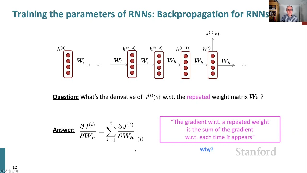
00:11:48.000 | But the central bit that's a little bit different and is more complicated is that we have this WH matrix that runs along the sequence that we keep on applying to update our hidden state.

00:12:05.000 | So what's the derivative of JT of theta with respect to the repeated weight matrix WH?

00:12:13.000 | And well, the answer to that is that what we do is we look at it in each position.

00:12:22.000 | And work out what the partials are of JT with respect to WH in position one or position two, position three, position four, etc.

00:12:35.000 | Right along the sequence. And we just sum up all of those partials. And that gives us a partial for JT with respect to WH overall.

00:12:46.000 | So the answer for a current neural networks is the gradient with respect to a repeated weight in our current network is the sum of the gradient with respect to each time it appears.

00:13:01.000 | And let me just then go through a little why that is the case. But before I do that, let me just note one gotcha.

00:13:11.000 | I mean, it's just not the case that this means it equals T times the partial of JT with respect to WH.

00:13:22.000 | Because we're using WH here, here, here, here, here through the sequence. And for each of the places we use it, there's a different upstream gradient that's being fed into it.

00:13:33.000 | So each of the values in this sum will be completely different from each other.

00:13:40.000 | Well, why we get this answer is essentially a consequence of what we talked about in the third lecture.

00:13:49.000 | So to take the simplest case of that, right, that if you have a multivariable function f of x, y,

00:13:57.000 | and you have two single variable functions, x of t and y of t, which are fed one input t.

00:14:05.000 | Well, then the simple version of working out the derivative of this function is you take the derivative down one path and you take the derivative down the other path.

00:14:18.000 | And so in the slides in lecture three, that was what was summarized on a couple of slides by the slogan, "gradient sum at outward branches."

00:14:30.000 | So T has outward branches. And so you take gradient here on the left, gradient on the right, and you sum them together.

00:14:39.000 | And so really what's happening with a recurrent neural network is just many pieces generalization of this.

00:14:47.000 | So we have one W.H. matrix and we're using it to keep on updating the hidden state at time one, time two, time three, right through time T.

00:14:58.000 | And so what we're going to get is that this has a lot of outward branches and we're going to sum the gradient path at each one of them.

00:15:12.000 | But what is this gradient path here? It kind of goes down here and then goes down there.

00:15:19.000 | But, you know, actually the bottom part is that we're just using W.H. at each position.

00:15:26.000 | So we have the partial of W.H. used at position i with respect to the partial of W.H., which is just our weight matrix for our recurrent neural network.

00:15:37.000 | So that's just one because, you know, we're just using the same matrix everywhere.

00:15:43.000 | And so we are just then summing the partials in each position that we use it.

00:15:52.000 | OK, practically, what does that mean in terms of how you compute this?

00:15:58.000 | Well, if you're doing it by hand, what happens is you start at the end, just like the general lecture three story.

00:16:08.000 | You work out derivatives with respect to the hidden layer and then with respect to W.H. at the last time step.

00:16:19.000 | And so that gives you one update for W.H. but then you continue passing the gradient back to the t minus one time step.

00:16:28.000 | And after a couple more steps of the chain rule, you get another update for W.H.

00:16:34.000 | and you simply sum that onto your previous update for W.H. and then you go to h t minus two.

00:16:41.000 | You get another update for W.H. and you sum that onto your update for W.H. and you go back all the way.

00:16:48.000 | And you sum up the gradients as you go. And that gives you a total update for W.H.

00:16:56.000 | And so there's sort of two tricks here. And I'll just mention the two tricks.

00:17:01.000 | You have to kind of separately sum the updates for W.H. and then once you've finished, apply them all at once.

00:17:09.000 | You don't want to actually be changing the W.H. matrix as you go, because that's then invalid,

00:17:14.000 | because the forward calculations were done with the constant W.H. that you had from the previous state all through the network.

00:17:25.000 | The second trick is, well, if you're doing this for sentences, you can normally just go back to the beginning of the sentence.

00:17:33.000 | But if you've got very long sequences, this can really slow you down if you're having to sort of run this algorithm back for a huge amount of time.

00:17:43.000 | So something people commonly do is what's called truncated backpropagation through time, where you choose some constant, say 20,

00:17:52.000 | and you say, well, I'm just going to run this backpropagation for 20 time steps, sum those 20 gradients, and then I'm just done.

00:18:01.000 | That's what I'll update the W.H. matrix with. And that works just fine.

00:18:10.000 | OK, so now, given a corpus, we can train simple RNN.

00:18:17.000 | And so that's good progress. But this is a model that can also generate text in general.

00:18:25.000 | So how do we generate text? Well, just like in our N-gram language model, we're going to generate text by repeated sampling.

00:18:34.000 | So we're going to start off with an initial state. And this slide is imperfect.

00:18:44.000 | So the initial state for the hidden state is normally just taken as a zero vector.

00:18:52.000 | And while then we need to have something for a first input. And on this slide, the first input is shown as the first word, my.

00:18:59.000 | And if you want to feed a starting point, you could feed my. But a lot of the time you'd like to generate a sentence from nothing.

00:19:07.000 | And if you want to do that, what's conventional is to additionally have a beginning of sequence token, which is a special token.

00:19:14.000 | So you'll feed in the beginning of sequence token in at the beginning as the first token.

00:19:19.000 | It has an embedding. And then you use the RNN update and then you generate using the softmax and next word.

00:19:28.000 | And while you generate a probability distribution over next words, and then at that point you sample from that and it chooses some word like favorite.

00:19:40.000 | And so then the trick is for doing generation that you take this word that you sampled and you copy it back down to the input and then you feed it in as an input.

00:19:51.000 | Next step, if you are an N sample from the softmax, get another word and just keep repeating this over and over again.

00:19:59.000 | And you start generating the text and how you end is as well as having a beginning of sequence special symbol.

00:20:09.000 | You usually have an end of sequence special symbol. And at some point, the recurrent neural network will generate the end of sequence symbol.

00:20:19.000 | And then you say, OK, I'm done. I'm finished generating text.

00:20:25.000 | So before going on for the more of the difficult content of the lecture, we can just have a little bit of fun with this and try training up and generating text with a recurrent neural network model.

00:20:39.000 | So you can generate you can train an RNN on any kind of text.

00:20:43.000 | And so that means one of the fun things that you can do is generate text in different styles based on what you could train it from.

00:20:54.000 | So here, Harry Potter is a there is a fair amount of a corpus of text.

00:21:00.000 | So you can train an RNN LM on the Harry Potter books and then say, go off and generate some text and it'll generate text like this.

00:21:08.000 | Sorry, how Harry shouted, panicking. I'll leave those brooms in London. Are they?

00:21:14.000 | No idea, said nearly headless Nick, casting low close by Cedric, carrying the last bit of treacle charms from Harry's shoulder.

00:21:21.000 | And to answer him, the common room perched upon it. Four arms held a shining knob from when the spider hadn't felt it seemed he reached the teams, too.

00:21:31.000 | Well, so on the one hand, that's still kind of a bit incoherent as a story.

00:21:37.000 | On the other hand, it's sort of sounds like Harry Potter and certainly the kind of, you know, vocabulary and constructions it uses.

00:21:45.000 | And I think you'd agree that, you know, even though it gets sort of incoherent, it's sort of more coherent than what we got from an N-gram language model.

00:21:55.000 | When I showed a generation in the last lecture, you can choose a very different style of text.

00:22:04.000 | So you could instead train the model on a bunch of cookbooks.

00:22:09.000 | And if you do that, you can then say generate based on what you've learned about cookbooks and it'll just generate a recipe.

00:22:17.000 | So here's a recipe. Chocolate ranch barbecue. Categories yield six servings.

00:22:25.000 | Two tablespoons of Parmesan cheese chopped. One cup of coconut milk. Three eggs beaten.

00:22:32.000 | Place each pasta over layers of lumps. Shape mixture into the moderate oven and simmer until firm.

00:22:39.000 | Serve hot and bodied fresh mustard, orange and cheese. Combine the cheese and salt together.

00:22:46.000 | The dough in a large skillet. Add the ingredients and stir in the chocolate and pepper.

00:22:52.000 | So, you know, this recipe makes no sense and it's sufficiently incoherent.

00:22:58.000 | There's actually even no danger that you'll try cooking this at home.

00:23:02.000 | But, you know, something that's interesting is although, you know, this really just isn't a recipe and the things that are done in the instructions have no relation to the ingredients,

00:23:17.000 | that the thing that's interesting that it has learned is this recurrent neural network model is that it's really mastered the overall structure of a recipe.

00:23:27.000 | It knows the recipe has a title. It often tells you about how many people it serves.

00:23:33.000 | It lists the ingredients and then it has instructions to make it.

00:23:37.000 | So that's sort of fairly impressive in some sense, the high level text structuring.

00:23:44.000 | So the one other thing I wanted to mention was when I say you can train an RNN language model on any kind of text.

00:23:52.000 | The other difference from where we were in N-gram language models was on N-gram language models that just meant counting N-grams and meant it took two minutes,

00:24:02.000 | even on a large corpus with any modern computer. Training your RNN LM actually can then be a time intensive activity and you can spend hours doing that,

00:24:12.000 | as you might find next week when you're training machine translation models.

00:24:18.000 | OK, how do we decide if our models are good or not?

00:24:26.000 | So the standard evaluation metric for language models is what's called perplexity.

00:24:33.000 | And what perplexity is, is kind of like when you were training your model, you use teacher forcing over a piece of text that's a different piece of text,

00:24:49.000 | which isn't text that was in the training data. And you say, well, given a sequence of T words,

00:24:57.000 | what probability do you give to the actual T plus one word? And you repeat that at each position.

00:25:05.000 | And then you take the inverse of that probability and raise it to the one on T for the length of your test text sample.

00:25:14.000 | And that number is the perplexity. So it's a geometric mean of the inverse probabilities.

00:25:22.000 | Now, after that explanation, perhaps an easier way to think of it is that the perplexity is simply the cross entropy loss that I introduced before exponentiated.

00:25:38.000 | So, but, you know, it's now the other way around. So low perplexity is better.

00:25:46.000 | So there's actually an interesting story about these perplexities. So a famous figure in the development of probabilistic and machine learning approaches to natural language processing is Fred Jelinek,

00:25:59.000 | who died a few years ago, and he was trying to interest people in the idea of using probability models and machine learning for natural language processing at a time.

00:26:15.000 | This is the 1970s and early 1980s, when nearly everyone in the field of AI was still in the thrall of logic based models and blackboard architectures and things like that for artificial intelligence systems.

00:26:31.000 | And so Fred Jelinek was actually an information theorist by background, and who then got interested in working with speech and then language data.

00:26:44.000 | So at that time, the stuff that's this sort of exponential or using cross entropy losses was completely bread and butter to Fred Jelinek,

00:26:55.000 | but he'd found that no one in AI could understand the bottom half of the slide.

00:27:01.000 | And so he wanted to come up with something simple that AI people at that time could understand.

00:27:07.000 | And perplexity has a kind of a simple interpretation you can tell people. So if you get a perplexity of 53, that means how uncertain you are of the next word is equivalent to the uncertainty of that you're tossing a 53 sided dice and it coming up as a one.

00:27:31.000 | Right. So that was kind of an easy, simple metric. And so he introduced that idea.

00:27:40.000 | But, you know, I guess things stick. And to this day, everyone evaluates their language models by providing perplexity numbers. And so here are some perplexity numbers.

00:27:52.000 | So traditional Ngram language models commonly had perplexities over 100. But if you made them really big and really careful, you carefully you could get them down into a number like 67.

00:28:06.000 | As people started to build more advanced recurrent neural networks, especially as they moved beyond the kind of simple RNNs, which is all I've shown you so far, which one of is in the second line of the slide into LSTMs, which I talk about later in this course,

00:28:26.000 | that people started producing much better perplexities. And here we're getting perplexities down to 30. And this is results actually from a few years ago. So nowadays people get perplexities of even lower than 30.

00:28:42.000 | So you have to be realistic in what you can expect, right? Because if you're just generating a text, some words are almost determined.

00:28:52.000 | So, you know, if it's something like, you know, Sue gave the man a napkin, he said, "Thank," you know, basically 100% you should be able to say the word that comes next is "you."

00:29:06.000 | You can predict really well. But, you know, if it's a lot of other sentences, like, "He looked out the window and saw something," right? No probability in the model or model in the world can give a very good estimate of what's actually going to be coming next at that point.

00:29:23.000 | And so that gives us the sort of residual uncertainty that leads to perplexities that on average might be around 20 or something.

00:29:33.000 | Okay. So we've talked a lot about language models now. Why should we care about language modeling?

00:29:41.000 | You know, well, there's sort of an intellectual scientific answer that says this is a benchmark task, right?

00:29:49.000 | If what we want to do is build machine learning models of language and our ability to predict what word will come next in the context, that shows how well we understand both the structure of language and the structure of the human world that language talks about.

00:30:07.000 | But there's a much more practical answer than that, which is, you know, language models are really the secret tool of natural language processing.

00:30:18.000 | So if you're talking to any NLP person and you've got almost any task, it's quite likely they'll say, "Oh, I bet we could use a language model for that."

00:30:32.000 | And so language models are sort of used as not the whole solution, but a part of almost any task.

00:30:41.000 | Any task that involves generating or estimating the probability of text. So you can use it for predictive typing, speech recognition, grammar correction, identifying authors, machine translation, summarization, dialogue, just about anything you do with natural language involves language models.

00:31:00.000 | And we'll see examples of that in following classes, including next Tuesday, where we're using language models for machine translation.

00:31:10.000 | OK, so a language model is just a system that predicts the next word.

00:31:16.000 | A recurrent neural network is a family of neural networks which can take sequential input of any length.

00:31:25.000 | They reuse the same weights to generate a hidden state and optionally, but commonly, an output on each step.

00:31:33.000 | Note that these two things are different.

00:31:37.000 | So we've talked about two ways that you could build language models, but one of them is RNNs being a great way. But RNNs can also be used for a lot of other things.

00:31:48.000 | So let me just quickly preview a few of the things you can do with RNNs.

00:31:53.000 | So there are lots of tasks that people want to do in NLP, which are referred to as sequence tagging tasks, where we'd like to take words of text and do some kind of classification along the sequence.

00:32:07.000 | So one simple common one is to give words parts of speech. That is a determiner, startled is an adjective, cat is a noun, knocked is a verb.

00:32:17.000 | And well, you can do this straightforwardly by using a recurrent neural network as a sequential classifier, where it's now going to generate parts of speech rather than the next word.

00:32:32.000 | You can use a recurrent neural network for sentiment classification. Well, this time we don't actually want to generate an output at each word necessarily, but we want to know what the overall sentiment looks like.

00:32:46.000 | So somehow we want to get out a sentence encoding that we can perhaps put through another neural network layer to judge whether the sentence is positive or negative.

00:32:57.000 | Well, the simplest way to do that is to think, well, after I've run my LSTM through the whole sentence, actually this final hidden state, it's encoded the whole sentence.

00:33:12.000 | Because remember, I updated that hidden state based on each previous word. And so you could say that this is the whole meaning of the sentence.

00:33:20.000 | So let's just say that is the sentence encoding and then put an extra classifier layer on that with something like a softmax classifier.

00:33:31.000 | That method has been used and it actually works reasonably well. And if you sort of train this model end to end, well, it's actually then motivated to preserve sentiment information in the hidden state of the recurrent neural network,

00:33:45.000 | because that will allow it to better predict the sentiment of the whole sentence, which is the final task and hence loss function that we're giving the network.

00:33:55.000 | But it turns out that you can commonly do better than that by actually doing things like feeding all hidden states into the sentence encoding, perhaps by making the sentence encoding an element-wise max or an element-wise mean of all the hidden states.

00:34:14.000 | Because this then more symmetrically encodes the hidden state over each time step. Another big use of recurrent neural networks is what I'll call language encoder module uses.

00:34:33.000 | So any time you have some text, for example, here we have a question of what nationality was Beethoven, we'd like to construct some kind of neural representation of this.

00:34:46.000 | So one way to do it is to run a recurrent neural network over it. And then just like last time, to either take the final hidden state or take some kind of function of all the hidden states and say that's the sentence representation.

00:35:05.000 | And we could do the same thing for the context. So for question answering, we're going to build some more neural net structure on top of that.

00:35:14.000 | And we'll learn more about that in a couple of weeks when we have the question answering lecture.

00:35:19.000 | But the key thing is what we built so far, we used to get sentence representation. So it's a language encoder module.

00:35:28.000 | So that was the language encoding part. We can also use RNNs to decode into language. And that's commonly used in speech recognition, machine translation, summarization.

00:35:42.000 | So if we have a speech recognizer, the input is an audio signal. And what we want to do is decode that into language.

00:35:50.000 | Well, what we could do is use some function of the input, which is probably itself going to be a neural net, as the initial hidden state of our RNN LM.

00:36:05.000 | And then we say start generating text based on that. And so it should then we generate word at a time by the method that we just looked at.

00:36:15.000 | We turn the speech into text. So this is an example of a conditional language model because we're now generating text conditioned on the speech signal.

00:36:26.000 | And a lot of the time you can do interesting, more advanced things with recurrent neural networks by building conditional language models.

00:36:36.000 | Another place you can use conditional language models is for text classification tasks, including sentiment classification.

00:36:44.000 | So if you can condition your language model based on a kind of sentiment, you can build a kind of classifier for that.

00:36:53.000 | And another use that we'll see a lot of next class is for machine translation.

00:36:59.000 | OK, so that's the end of the intro to.

00:37:06.000 | Doing things with recurrent neural networks and language models.

00:37:10.000 | Now I want to move on and tell you about the fact that everything is not perfect and these recurrent neural networks tend to have a couple of problems.

00:37:22.000 | And we'll talk about those and then in part that will then motivate coming up with a more advanced recurrent neural network architecture.

00:37:31.000 | So the first problem to be mentioned is the idea of what's called vanishing gradients.

00:37:39.000 | And what does that mean? Well, at the end of our sequence, we have some overall loss that we're calculating.

00:37:48.000 | And well, what we want to do is back propagate that loss and we want to back propagate it right along the sequence.

00:37:57.000 | And so we're working out the partials of J4 with respect to the hidden state at time one.

00:38:05.000 | And when we have a longer sequence, we'll be working out the partials of J20 with respect to the hidden state at time one.

00:38:12.000 | And how do we do that?

00:38:14.000 | Well, how we do it is by composition in the chain rule.

00:38:19.000 | We've got a big long chain rule along the whole sequence.

00:38:25.000 | Well, if we're doing that, you know, we're multiplying a ton of things together.

00:38:33.000 | And so the danger of what tends to happen is that as we do these multiplications, a lot of time, these partials between successive hidden states become small.

00:38:49.000 | And so what happens is as we go along, the gradient gets smaller and smaller and smaller and starts to peter out.

00:38:58.000 | And to the extent that it peters out, well, then we've kind of got no upstream gradient and therefore we won't be changing the parameters at all.

00:39:09.000 | And that turns out to be pretty problematic.

00:39:14.000 | So the next couple of slides sort of say a little bit about the why and how this happens.

00:39:24.000 | What's presented here is a kind of only semi-formal wave your hands at the kind of problems that you might expect.

00:39:34.000 | If you really want to sort of get into all the details of this, you should look at the couple of papers that are mentioned in small print at the bottom of the slide.

00:39:43.000 | But at any rate, if you remember that this is our basic recurrent neural network equation.

00:39:50.000 | Well, let's consider an easy case. Suppose we sort of get rid of our non-linearity and just assume that it's an identity function.

00:40:00.000 | OK, so then when we're working out the partials of the hidden state with respect to the previous hidden state, we can work those out in the usual way, according to the chain rule.

00:40:13.000 | And then if sigma is simply the identity function, well, then everything gets really easy for us.

00:40:23.000 | So only the sigma just goes away and only the first term involves h at time t minus one.

00:40:33.000 | So the later terms go away. And so our gradient ends up as wh.

00:40:41.000 | Well, that's doing it for just one time step. What happens when you want to work out these partials a number of time steps away?

00:40:49.000 | So we want to work it out the partial of time step i with respect to j.

00:40:59.000 | Well, what we end up with is a product of the partials of successive time steps.

00:41:07.000 | And well, each of those is coming out as wh. And so we end up getting wh raised to the lth power.

00:41:21.000 | And well, our potential problem is that if wh is small in some sense, then this term gets exponentially problematic.

00:41:30.000 | It becomes vanishingly small as our sequence length becomes long.

00:41:36.000 | Well, what can we mean by small? Well, a matrix is small if its eigenvalues are all less than one.

00:41:44.000 | So we can rewrite what's happening with this successive multiplication using eigenvalues and eigenvectors.

00:41:53.000 | And I should say that all eigenvalues less than one is a sufficient but not necessary condition for what I'm about to say.

00:42:01.000 | Right. So we can rewrite things using the eigenvectors as a basis.

00:42:08.000 | And if we do that, we end up getting the eigenvalues being raised to the lth power.

00:42:17.000 | And so if all of our eigenvalues are less than one, if we're taking a number less than one and raising it to the lth power,

00:42:26.000 | that's going to approach zero as the sequence length grows. And so the gradient vanishes.

00:42:33.000 | OK, now the reality is more complex than that, because actually we always use a nonlinear activation sigma.

00:42:40.000 | But, you know, in principle, it's sort of the same thing. Apart from we have to consider in the effect of the nonlinear activation.

00:42:51.000 | OK, so why is this a problem that the gradients disappear?

00:42:55.000 | Well, suppose we're wanting to look at the influence of time steps well in the future on the representations we want to have early in the sentence.

00:43:08.000 | Well, what's happening late in the sentence just isn't going to be giving much information about what we should be storing in the h at time one vector.

00:43:21.000 | Whereas on the other hand, the loss at time step two is going to be giving a lot of information at what should be stored in the hidden vector at time step one.

00:43:33.000 | So the end result of that is that what happens is that these simple RNNs are very good at modelling nearby effects,

00:43:45.000 | but they're not good at all at modelling long term effects because the gradient signal from far away is just lost too much.

00:43:54.000 | And therefore, the model never effectively gets to learn what information from far away it would be useful to preserve into the future.

00:44:06.000 | So let's consider that concretely for the example of language models that we've worked on.

00:44:12.000 | So here's a piece of text. When she tried to print her tickets, she found that the printer was out of toner.

00:44:20.000 | She went to the stationery store to buy more toner. It was very overpriced.

00:44:25.000 | After installing the toner into the printer, she finally printed her.

00:44:29.000 | And, well, you're all smart human beings. I trust you can all guess what the word that comes next is.

00:44:35.000 | It should be tickets. But, well, the problem is that for the RNN to start to learn cases like this,

00:44:44.000 | it would have to carry through in its hidden state a memory of the word tickets for sort of whatever it is, about 30 hidden state updates.

00:44:55.000 | And, well, we'll train on this example. And so we'll be wanting it to predict tickets as the next word.

00:45:04.000 | And so a gradient update will be sent right back through the hidden states of the LSTM corresponding to this sentence.

00:45:13.000 | And that should tell the model it's good to preserve information about the word tickets because that might be useful in the future.

00:45:22.000 | Here it was useful in the future. But the problem is that the gradient signal will just become far too weak after a bunch of words.

00:45:33.000 | And it just never learns that dependency. And so what we find in practice is the model is just unable to predict similar long distance dependencies at test time.

00:45:45.000 | I've spent quite a long time on vanishing gradients and really vanishing gradients are the big problem in practice with using recurrent neural networks over long sequences.

00:46:01.000 | But, you know, I have to do justice to the fact that you can actually also have the opposite problem.

00:46:06.000 | You can also have exploding gradients. So if a gradient becomes too big, that's also a problem.

00:46:15.000 | And it's a problem because the stochastic gradient update step becomes too big. Right.

00:46:23.000 | So remember that our parameter update is based on the product of the learning rate and the gradient.

00:46:30.000 | So if your gradient is huge, right, you've calculated, oh, it's got a lot of slope here.

00:46:36.000 | This has a slope of ten thousand. Then your parameter update can be arbitrarily large.

00:46:45.000 | And that's potentially problematic. That can cause a bad update where you take a huge step and you end up at a weird and bad parameter configuration.

00:46:56.000 | So you sort of think you're coming up with a to a steep hill to climb.

00:47:01.000 | And while you want to be climbing the hill to high likelihood, that actually the gradient is so steep that you make an enormous update.

00:47:11.000 | And then suddenly your parameters are over an hour and you've lost your hill altogether.

00:47:16.000 | There's also the practical difficulty that we only have so much resolution now, floating point numbers.

00:47:21.000 | So if your gradient gets too steep, you start getting not a numbers in your calculations, which ruin all your hard training work.

00:47:32.000 | We use a kind of an easy fix to this, which is called gradient clipping, which is we choose some reasonable number.

00:47:42.000 | And we say we're just not going to deal with gradients that are bigger than this number.

00:47:47.000 | A commonly used number is 20. You know, something that's got a range of spread, but not that high.

00:47:53.000 | You know, you can use ten or hundred somewhere sort of in that range.

00:47:58.000 | And if the norm of the gradient is greater than that threshold, we simply just scale it down, which means that we then make a smaller gradient update.

00:48:10.000 | So we're still moving in exactly the same direction, but we're taking a smaller step.

00:48:17.000 | So doing this gradient clipping is important, you know, but it's an easy problem to solve.

00:48:27.000 | OK, so the thing that we've still got left to solve is how to really solve this problem of vanishing gradients.

00:48:39.000 | So the problem is, yeah, these RNNs just can't preserve information over many time steps.

00:48:47.000 | And one way to think about that intuitively is at each time step, we have a hidden state.

00:48:56.000 | And the hidden state is being completely changed at each time step.

00:49:02.000 | And it's being changed in a multiplicative manner by multiplying by WH and then putting it through non-linearity.

00:49:13.000 | Like maybe we could make some more progress if we could more flexibly maintain a memory in our recurrent neural network,

00:49:26.000 | which we can manipulate in a more flexible manner that allows us to more easily preserve information.

00:49:35.000 | And so this was an idea that people started thinking about.

00:49:39.000 | And actually, they started thinking about it a long time ago in the late 1990s.

00:49:48.000 | And Hochreid and Schmidhuber came up with this idea that got called long short term memory RNNs as a solution to the problem of vanishing gradients.

00:50:01.000 | I mean, so this 1997 paper is the paper you always see cited for LSTMs.

00:50:07.000 | But, you know, actually, in terms of what we now understand as an LSTM, it was missing part of it.

00:50:15.000 | In fact, it's missing what in retrospect has turned out to be the most important part of the modern LSTM.

00:50:24.000 | So really, in some sense, the real paper that the modern LSTM is due to is this slightly later paper by Gersh, Schmidhuber and Cummins from 2000,

00:50:36.000 | which additionally introduces the forget gate that I'll explain in a minute.

00:50:42.000 | Yeah, so so this was some very clever stuff that was introduced and turned out later to have an enormous impact.

00:50:52.000 | If I just diverge from the technical part for one more moment, that, you know,

00:50:59.000 | for those of you who these days think that mastering your networks is the path to fame and fortune.

00:51:08.000 | The funny thing is, you know, at the time that this work was done, that just was not true.

00:51:15.000 | Right. Very few people were interested in neural networks.

00:51:19.000 | And although long, short term memories have turned out to be one of the most important, successful and influential ideas in neural networks for the following 25 years,

00:51:32.000 | really, the original authors didn't get recognition for that.

00:51:36.000 | So both of them are now professors at German universities.

00:51:41.000 | But Hochreiter moved over into doing bioinformatics work to find something to do.

00:51:50.000 | And Gersh actually is doing kind of multimedia studies.

00:51:55.000 | So that's the fates of history.

00:52:00.000 | OK, so what is an LSTM?

00:52:03.000 | So the crucial innovation of an LSTM is to say, well, rather than just having one hidden vector in the recurrent model,

00:52:15.000 | we're going to build a model with two hidden vectors at each time step,

00:52:24.000 | one of which is still called the hidden state H and the other of which is called the cell state.

00:52:32.000 | Now, you know, arguably in retrospect, these were named wrongly because as you'll see, when we look at it in more detail,

00:52:40.000 | in some sense, the cell is more equivalent to the hidden state of the simple RNN than vice versa.

00:52:46.000 | But we're just going with the names that everybody uses. So both of these are vectors of length N.

00:52:53.000 | And it's going to be the cell that stores long term information.

00:52:58.000 | And so we want to have something that's more like memory. So the meaning like RAM in the computer.

00:53:06.000 | So the cell is designed so you can read from it, you can erase parts of it and you can write new information to the cell.

00:53:16.000 | And the interesting part of an LSTM is then it's got control structures to decide how you do that.

00:53:24.000 | So the selection of which information to erase, write and read is controlled by probabilistic gates.

00:53:31.000 | So the gates are also vectors of length N. And on each time step, we work out a state for the gate vectors.

00:53:41.000 | So each element of the gate vectors is a probability. So they can be open probability one,

00:53:46.000 | closed probability zero or somewhere in between. And their value will be saying how much do you erase?

00:53:54.000 | How much do you write? How much do you read? And so these are dynamic gates with a value that's computed based on the current context.

00:54:06.000 | OK, so in this next slide, we go through the equations of an LSTM.

00:54:11.000 | But following this, there are some more graphic slides which will probably be easier to absorb.

00:54:17.000 | Right. So we again, just like before, it's a recurrent neural network.

00:54:21.000 | We have a sequence of inputs X, T and we're going to at each time step compute a cell state and a hidden state.

00:54:30.000 | So how do we do that? So firstly, we're going to compute values of the three gates.

00:54:38.000 | And so we're computing the gate values using an equation that's identical to the equation for the simple recurrent neural network.

00:54:49.000 | But in particular, oops, sorry, I'll just say what the gates are first.

00:54:55.000 | So there's a forget gate which we will control what is kept in the cell at the next time step versus what is forgotten.

00:55:05.000 | There's an input gate which is going to determine which parts of a calculated new cell content get written to the cell memory.

00:55:14.000 | And there's an output gate which is going to control what parts of the cell memory are moved over into the hidden state.

00:55:21.000 | And so each of these is using the logistic function because we want them to be in each element of this vector,

00:55:30.000 | a probability which will say whether to fully forget, partially forget or fully remember.

00:55:39.000 | Yeah. And the equation for each of these is exactly like the simple R and N equation.

00:55:44.000 | But note, of course, that we've got different parameters for each one.

00:55:48.000 | So we've got forgetting weight matrix W with a forgetting bias and a forgetting multiplier of the input.

00:56:01.000 | OK, so then we have the other equations that really are the mechanics of the LSTM.

00:56:09.000 | So we have something that will calculate a new cell content.

00:56:14.000 | So this is our candidate update. And so for calculating the candidate update,

00:56:20.000 | we're again essentially using exactly the same simple R and N equation.

00:56:26.000 | Apart from now, it's usual to use tanh. So you get something that, as discussed last time, is balanced around zero.

00:56:34.000 | OK, so then to actually update things, we use our gates.

00:56:40.000 | So for our new cell content, what the idea is, is that we want to remember some,

00:56:47.000 | but probably not all of what we had in the cell from previous time steps.

00:56:52.000 | And we want to store some, but probably not all of the value that we've calculated as the new cell update.

00:57:04.000 | And so the way we do that is we take the previous cell content and then we take its Hadamard product with the forget vector.

00:57:17.000 | And then we add to it the Hadamard product of the input gate times the candidate cell update.

00:57:30.000 | And then for working out the new hidden state, we then work out which parts of the cell to expose in the hidden state.

00:57:41.000 | And so after taking a tanh transform of the cell, we then take the Hadamard product with the output gate.

00:57:49.000 | And that gives us our hidden representation.

00:57:52.000 | And it's this hidden representation that we then put through a softmax layer to generate our next output of our LSTM recurrent neural network.

00:58:03.000 | Yeah. So the gates and the things that they're put with are vectors of size n.

00:58:13.000 | And what we're doing is we're taking each element of them and multiplying them element wise to work out a new vector.

00:58:21.000 | And then we get two vectors and that we're adding together. So this way of doing things element wise,

00:58:28.000 | you sort of don't really see in standard linear algebra course. It's referred to as the Hadamard product.

00:58:36.000 | It's represented by some kind of circle. I mean, actually, in more modern work,

00:58:40.000 | it's been more usual to represent it with this slightly bigger circle with the dot at the middle as the Hadamard product symbol.

00:58:48.000 | And someday I'll change these slides to be like that. But I was lazy in redoing the equations.

00:58:54.000 | But the other notation you do see quite often is just using the same little circle that you use for function composition to represent Hadamard product.

00:59:04.000 | OK, so all of these things are being done as vectors of the same length n.

00:59:10.000 | And the other thing that you might notice is that the candidate update and the forget input and output gates all have a very similar form.

00:59:24.000 | The only difference is three logistics and one tanh. And none of them depend on each other.

00:59:30.000 | So all four of those can be calculated in parallel. And if you want to have an efficient LSTM implementation, that's what you do.

00:59:39.000 | OK, so here's the more graphical presentation of this.

00:59:43.000 | So these pictures come from Chris Ola. And I guess he did such a nice job at producing pictures for LSTMs that almost everyone uses them these days.

00:59:55.000 | And so this sort of pulls apart the computation graph of an LSTM unit.

01:00:02.000 | So blowing this up, you've got from the previous time step, both your cell and hidden recurrent vectors.

01:00:14.000 | And so you feed the hidden vector from the previous time step and the new input XT into the computation of the gates, which is happening down the bottom.

01:00:27.000 | So you compute the forget gate and then you use the forget gate in a Hadamard product here drawn as a actually a time symbol to forget some cell content.

01:00:39.000 | You work out the input gate and then using the input gate and a regular recurrent neural network like computation, you can compute candidate new cell content.

01:00:54.000 | And so then you add those two together to get the new cell content, which then heads out as the new cell content at time T.

01:01:05.000 | But then you also have worked out an output gate. And so then you take the cell content, put it through another non-linearity and Hadamard product it with the output gate.

01:01:21.000 | And that then gives you the new hidden state. So this is all kind of complex.

01:01:29.000 | But as to understanding why something is different is happening here.

01:01:34.000 | The thing to notice is that the cell state from T minus one is passing right through this to be the cell state at time T without very much happening to it.

01:01:49.000 | So some of it is being deleted by the forget gate and then some new stuff is being written to it as a result of using this candidate new cell content.

01:02:04.000 | But the real secret of the LSTM is that new stuff is just being added to the cell with an addition.

01:02:16.000 | Right. So in the simple RNN at each successive step, you are doing a multiplication and that makes it incredibly difficult to learn to preserve information in the hidden state over a long period of time.

01:02:32.000 | It's not completely impossible, but it's a very difficult thing to learn. Whereas with this new LSTM architecture, it's trivial to preserve information in the cell from one time step to the next.

01:02:46.000 | You just don't forget it. And it'll carry right through with perhaps some new stuff added in to also remember.

01:02:55.000 | And so that's the sense in which the cell behaves much more like RAM in a conventional computer that storing stuff and extra stuff can be stored into it and other stuff can be deleted from it as you go along.

01:03:12.000 | Okay, so the LSTM architecture makes it much easier to preserve information from many time steps.

01:03:21.000 | Right. So in particular, standard practice with LSTMs is to initialize the forget gate to a one vector, which it's just so that the starting point is to say preserve everything from previous time steps.

01:03:39.000 | And then it is then learning when it's appropriate to forget stuff.

01:03:45.000 | And in contrast, it's very hard to get a simple RNN to preserve stuff for a very long time.

01:03:53.000 | I mean, what does that actually mean?

01:03:56.000 | Well, you know, I've put down some numbers here. I mean, you know, what you get in practice, you know, depends on a million things.

01:04:05.000 | It depends on the nature of your data and how much data you have and what dimensionality your hidden states are. Blurdy, blurdy, blur.

01:04:14.000 | But just to give you some idea of what's going on is typically if you train a simple recurrent neural network that its effect of memory, its ability to be able to use things in the past to condition the future goes for about seven time steps.

01:04:31.000 | You just really can't get it to remember stuff further back in the past than that.

01:04:36.000 | Whereas for the LSTM, it's not complete magic. It doesn't work forever.

01:04:44.000 | But, you know, it's effectively able to remember and use things from much, much further back.

01:04:50.000 | So typically you find that with an LSTM, you can effectively remember and use things about a hundred time steps back. And that's just enormously more useful for a lot of the natural language understanding tasks that we want to do.

01:05:08.000 | And so that was precisely what the LSTM was designed to do.

01:05:13.000 | And I mean, so in particular, just going back to its name, quite a few people misparsed its name.

01:05:19.000 | The idea of its name was there's a concept of short term memory, which comes from psychology, and it had been suggested for simple RNNs that the hidden state of the RNN could be a model of human short term memory.

01:05:35.000 | And then there would be something somewhere else that would deal with human long term memory.

01:05:41.000 | But, well, people had found that this only gave you a very short, short term memory.

01:05:47.000 | So what Hochreiter and Schmidhuber were interested in was how we could give construct models with a long short term memory. And so that then gave us this name of LSTM.

01:06:03.000 | LSTMs don't guarantee that there are no vanishing or exploding gradients, but in practice, they provide, they don't tend to explode nearly the same way.

01:06:15.000 | Again, that plus sign is crucial rather than a multiplication. And so they're a much more effective way of learning long distance dependencies.

01:06:25.000 | Okay. So despite the fact that LSTMs were developed around 1997-2000, it was really only in the early 2010s that the world woke up to them and how successful they were.

01:06:42.000 | So it was really around 2013-2015 that LSTMs sort of hit the world, achieving state of the art results on all kinds of problems.

01:06:54.000 | One of the first big demonstrations was for handwriting recognition, then speech recognition, but then going on to a lot of natural language tasks, including machine translation, parsing, vision and language tasks like image captioning, as well, of course,

01:07:11.000 | using them for language models. And around these years, LSTMs became the dominant approach for most NLP tasks.

01:07:19.000 | The easiest way to build a good strong model was to approach the problem with an LSTM.

01:07:26.000 | So now in 2021, actually LSTMs are starting to be supplanted or have been supplanted by other approaches, particularly transformer models,

01:07:37.000 | which we'll get to in the class in a couple of weeks time. So this is the sort of picture you can see.

01:07:43.000 | So for many years, there's been a machine translation conference and sort of bake off competition called WMT, Workshop on Machine Translation.

01:07:53.000 | So if you look at the history of that, in WMT 2014, there was zero neural machine translation systems in the competition.

01:08:03.000 | 2014 was actually the first year that the success of LSTMs for machine translation was proven in a conference paper, but nothing occurred in this competition.

01:08:18.000 | By 2016, everyone had jumped on LSTMs as working great.

01:08:26.000 | And lots of people, including the winner of the competition, was using an LSTM model.

01:08:32.000 | If you then jump ahead to 2019, then there's relatively little use of LSTMs and the vast majority of people are now using transformers.

01:08:44.000 | So things change quickly in neural network land. And I keep on having to rewrite these lectures.

01:08:52.000 | So quick further note on vanishing and exploding gradients. Is it only a problem with recurrent neural networks?

01:09:00.000 | It's not. It's actually a problem that also occurs anywhere where you have a lot of depth, including feedforward and convolutional neural networks.

01:09:11.000 | Anytime when you've got long sequences of chain rules, which give you multiplications, the gradient can become vanishingly small as it back propagates.

01:09:22.000 | And so generally sort of lower layers are learned very slowly and are hard to train.

01:09:29.000 | So there's been a lot of effort in other places as well to come up with different architectures that let you learn more efficiently in deep networks.

01:09:42.000 | And the commonest way to do that is to add more direct connections that allow the gradient to flow.

01:09:49.000 | So the big thing in vision in the last few years has been ResNets, where the res stands for residual connections.

01:09:57.000 | And so the way they're made, this picture is upside down.

01:10:01.000 | So the input is at the top, is that you have these sort of two paths that are summed together.

01:10:09.000 | One path is just an identity path and the other one goes through some neural network layers.

01:10:14.000 | And so therefore, its default behavior is just to preserve the input, which might sound a little bit like what we just saw for LSTMs.

01:10:25.000 | There are other methods that then been dense nets where you add skip connections forward to every layer.

01:10:33.000 | Highway nets were also actually developed by Schmidhuber and sort of reminiscent of what was done with LSTMs.

01:10:41.000 | So rather than just having an identity connection as a ResNet has, it introduces an extra gate.

01:10:49.000 | So it looks more like an LSTM, which says how much to send the input through the highway versus how much to put it through a neural net layer.

01:11:00.000 | And those two are then combined into the output.

01:11:06.000 | So essentially, this problem occurs anywhere when you have a lot of depth in your layers of neural network.

01:11:15.000 | But it first arose and turns out to be especially problematic with recurrent neural networks.

01:11:23.000 | They're particularly unstable because of the fact that you've got this one weight matrix that you're repeatedly using through the time sequence.

01:11:35.000 | OK. So we've got we've got a couple of questions, more or less, about whether you would ever want to use an RNN, like a simple RNN instead of an LSTM.

01:11:49.000 | How does the LSTM learn what to do with its gates? Can you opine on those things?

01:11:55.000 | Sure. So I think basically the answer is you should never use a simple RNN these days.

01:12:04.000 | You should always use an LSTM. I mean, you know, obviously that depends on what you're doing.

01:12:10.000 | If you're wanting to do some kind of analytical paper or something, you might prefer a simple RNN.

01:12:17.000 | And it is the case that you can actually get decent results with simple RNNs, providing you're very careful to make sure that things aren't exploding nor vanishing.

01:12:33.000 | But, you know, in practice, getting simple RNNs to work and preserve long contexts is incredibly difficult where you can train LSTMs and they will just work.

01:12:44.000 | So really, you should always just use an LSTM. Now, wait, the second question was?

01:12:52.000 | I think there's a bit of confusion about like whether the gates are learning differently.

01:12:58.000 | Oh yeah. So the gates are also just learn. So if we go back to these equations.

01:13:08.000 | You know, this is the complete model. And when we're training the model, every one of these parameters, so all of these W, U and Bs, everything is simultaneously being trained by backprop.

01:13:25.000 | So that what you hope, and indeed it works, is the model is learning what stuff should I remember for a long time versus what stuff should I forget.

01:13:38.000 | What things in the input are important versus what things in the input don't really matter.

01:13:43.000 | So it can learn things like function words like "a" and "the" don't really matter, even though everyone uses them in English.

01:13:51.000 | So you can just not worry about those. So all of this is learned and the models do actually successfully learn gate values about what information is useful to preserve long term versus what information is really only useful short term for predicting the next one or two words.

01:14:11.000 | Finally, the gradient improvements due to the, so you said that the addition is really important between the new cell candidate and the cell state. I don't think at least a couple of students have sort of questioned that. So if you want to go over that again that might be useful.

01:14:28.000 | Sure. So what we would like is an easy way for memory to be preserved long term.

01:14:41.000 | And, you know, one way which is what ResNets use is just to sort of completely have a direct path from CT minus one to CT and will preserve entirely the history.

01:14:56.000 | So that's kind of there's a default action of preserving information about the past long term. LSTMs don't quite do that, but they allow that function to be easy.

01:15:10.000 | So you start off with the previous cell state, and you can forget some of it by the forget gate so you can delete stuff out of your memory that's a useful operation.

01:15:21.000 | And then while you're going to be able to update the content of the cell with this, the right operation that occurs in the plus, where depending on the input gate, some parts of what's in the cell will be added to, but you can think of that adding as overlaying

01:15:40.000 | extra information, everything that was in the cell that wasn't forgotten is still continuing on to the next time step.

01:15:50.000 | And in particular, when you're doing the back propagation through time that there isn't.

01:15:58.000 | I want to say there isn't a multiplication between CT and CT minus one, and there's this unfortunate time symbol here but remember that's the Hadamard product, which is zeroing out part of it with the forget gate.

01:16:11.000 | It's not a multiplication by a matrix, like in the simple RNN.

01:16:22.000 | I hope that's good.

01:16:24.000 | Okay, so there are a couple of other things that I wanted to get through before the end. I guess I'm not going to have time to do both of them I think so I'll do the last one probably next time.

01:16:35.000 | These are actually simple and easy things, but they complete our picture.

01:16:43.000 | So we, I sort of briefly alluded to this example of sentiment classification, where what we could do is run an RNN, maybe an LSTM over a sentence, call this our representation of the sentence, and you feed it into a softmax classifier to classify

01:17:04.000 | for sentiment. So what we're actually saying there is that we can regard the hidden state as a representation of a word in context, that below that we have just a word vector for terribly, but we then looked at our context and say okay we've now created a

01:17:29.000 | hidden state representation for the word terribly in the context of the movie was, and that proves to be a really useful idea, because words have different meanings in different contexts, but it seems like there's a defect of what we've done here, because our context only

01:17:49.000 | contains information from the left. What about right context, surely it also be useful to have the meaning of terribly depend on exciting, because often words mean different things based on what follows them.

01:18:05.000 | So, you know, if you have something like red wine, it means something quite different from a red light.

01:18:14.000 | So how can we deal with that. Well, an easy way to deal with that would be to say, well if we just want to come up with a neural encoding of a sentence, we could have a second RNN with completely separate parameters learned, and we can run it backwards

01:18:32.000 | through the sentence to get a backward representation of each word, and then we can get an overall representation of each word and context by just concatenating those two representations, and now we've got a representation of terribly that has both left and right

01:18:51.000 | context.

01:18:53.000 | So, we're simply running a forward RNN. And when I say RNN here. That just means any kind of recurrent neural network so commonly it'll be an LSTM, and a backward one.

01:19:07.000 | And then each time step we just concatenating their representations, with each of these having separate weights. And so then we regard this concatenated thing as the hidden state the contextual representation of a token at a particular time that we pass

01:19:26.000 | on to the model.

01:19:48.000 | So we're just concatenating their results at each time step, and that's what you're going to use later in the model.

01:19:56.000 | Okay, but, so, if you're doing an encoding problem like for sentiment classification or question answering.

01:20:07.000 | Using bi directional RNNs is a great thing to do.

01:20:11.000 | But they're only applicable if you have access to the entire input sequence.

01:20:17.000 | So, I'm not going to go into detail to language modeling, because in a language model necessarily you have to generate the next word, based on only the preceding context.

01:20:29.000 | But if you do have the entire input sequence that bi directionality gives you greater power. And indeed, that's been an idea that people have built on in subsequent work so when we get to transformers in a couple of weeks.

01:20:45.000 | We're going to spend a lot of time on the BERT model, where that acronym stands for bi directional encoder representations from transformers.

01:20:55.000 | So part of what's important in that model is the transformer, but really a central point of the paper was to say that you could build more powerful models using transformers by again, exploiting bi directionality.

01:21:13.000 | There's one teeny bit left on RNNs, but I'll sneak it into next class, and I'll call it the end for today.

01:21:20.000 | And if there are other things you'd like to ask questions about. You can find me on Nooks again in just a minute.

01:21:29.000 | Okay, so see you again next Tuesday.

01:21:33.000 | Transcribed by https://otter.ai

01:21:35.000 | you

Stanford CS224N NLP with Deep Learning | Winter 2021 | Lecture 6 - Simple and LSTM RNNs

Chapters