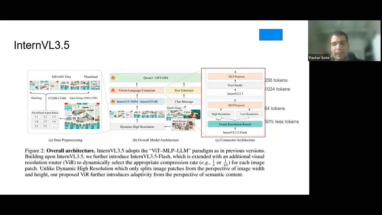
okay so hi everyone today i want to see inter bl 3.5 which is advanced open source multi-models in versatility reasoning and efficiency so the the why we choose this paper is because we wanted to have some open source multi-modality available to be able to compete with commercial model so every integration that you want to develop as an ai engineering now the bar or the standard will require to have multimodal capabilities so having this addition and see how it works is what it would be is is what will make you competing into the market so this this paper not only provides how they did it but also gives tips for the developer community to actually improve in their workflow in general so this paper is really good about it and so just things to keep in mind while i'm going through the slide the gray slides will be things that are not in the paper but i find it helpful to explain so we can kind of have something or have some baseline for explain what we what i saw in the papers and also i prepared a notebook for inference that will be referencing when when we when when we we need it so let me start here and also we will have breaks between sections so we kind of go over questions or ideas that you want to share so the overall idea is that you want have a multi-modality and these compose about text and image so you put your image you put your text so we wanted the image be process by this inter bl 3.5 and the text process to the language model or the language capability which in this case would be quen 3 and gpt open source and we wanted to be this versatile have reasoning capabilities and be efficiency and that's what this old paper is about so we are going to dissect those three core functionalities of the inter bl 3.5 so like i i just prepared this type of of of of this response so we can kind of understand what are the differences and you see we here we have four like four different type of response based on the different on the different models that they provide or at the different stage that that they provide at the model and you will understand that more in a bit but this is the response of pre-training and you will see the picture that i referenced to later but just keep in mind the different type of response this is a dog sitting on a rock in front of a building and the instruct model which is the next stage that they did is a fluffy white dog wearing a rainbow custom with a leech sitting on a rock surface under a clear blue sky with a shirt visible on the background and then the next stage for them was the order response that they provide for the next stage is smile white dog dressing a colorful rainbow alfie and wary bunny ears and standing on a rocky surface and you get the idea that they get different type of response at different stage and the reason why all sounds i mean reasonable within a picture of of of a dog in certain position is that the they initialize with the already language capabilities from the open source so even though that they might not understand fully the the the picture you might get the impression of a working solution so that's why they run a lot of experiments to actually understand if this is going somewhere or it was the the language making you believe that it was a reasonable answer without knowing the the the without really understanding the picture so yeah so i hope that would be helpful as introduction so let's go to the abstract and this the inter bl 3.5 which is a new family of open source multimodal models and the this advancing versatility reasoning capabilities and inference efficiency along the inter bl series and the key innovation that they did is that they add a cascade reinforcement learning framework which enhance reasoning through a two-stage process offline reinforcement learning for stable convergence and online reinforcement learning for refine alignment and you will see for me this was one of the most brilliant ideas that they provide and we will see this in detail and the other thing was that they proposed a visual resolution router and i was impressed by this because it's so simple but so effective that you can incorporate in your workflow web on whenever on whatever you are doing so it's one of those things that make you think why i didn't think about it or because it's so simple but it's so effective and that allows to dynamically adjust the resolution of visual tokens without compromising the performance and they also separate the vision from the language from the language from the language server so they deploy in in different parts is not in a sequence is is they running in parallel so they separate the vision and color from the language model across different gpus and this is what adds the the efficiency of the model in the training and the inference stage so yeah so those are the three core ideas enable reasoning through cascade reinforcement learning adjust dynamically the vision resolution token and separate the vision from the language model so this is kind of to give you an overview on on the overall performance and the key thing about this graph is that they are able to compete with the with the most or or the latest commercial models like gpt5 of gemini 2.5 pro but also the they they are able to do it across the different release that they did so you you see here that we have interview 3.5 app this is the the the most advanced model that they released but they release but they release also other models which gives flexibility to developer to use in in different in in different areas or in different settings using different computational capabilities so this is one of the of the of the of the advantage of this paper okay so they they have three main contributions so the first one is the release of the inter bl 3.5 series and through our series of models that goes from 1 billion to 241 billion and in both dense and mixture or of expert models also they include cascade reinforcement learning and the visual resolution router router and the couple visual from the language deployment and also they are able to compete with the commercial models available like gpt like gpt5 so this is was the main addition that they have so any questions so far about the introduction okay okay so let me go through the architecture so this is where we are going to spend the most amount of of time on this on this on this on this discussion and you see in the middle that we have the core architecture of of inter bl 3.5 and as as you can see we have on the size we have a close up to through two different things one is the dynamic high resolution and the other one is from the visual language connector so essentially what we are doing here is is that is that we are processing the image so we have an image and and we process that image image and based on the on the height and width of the image we we process that image into a predefined aspect ratio so we we don't process any image with the rate with the with a with their initial high-end width but we process and we use our predefined height and width based on on on on what they did and let me show you what i mean by that in this notebook okay so can you see the notebook right okay so you you here you see we put the image and we have this function that is find the closest aspiration so it doesn't have any intelligence it just look your width and height of of of of your image and based on that it has the dynamic processing which is the we which is those those predefined aspect ratio that that i provided you and at the end we provide a process image so i use a picture of my dog which is the one that i show you at the beginning so you can see the blue sky you can see it has a a a rain a rainbow custom and it has this is the building or the church in the back and when we process this image we process the image and we go through patches and those patches are with predefined aspect ratio that we that that i will show you on this dynamic high resolution okay so we pass the image now we know what is a predefined aspect ratio and there is no intelligence in that it's just a bunch of if and else statement and it defines what's the closest ratio and based on that now that we process the image we can put it into the vision capabilities of of the of of the model so we can translate to a more to to to to go through the llms but before we go through the llm we need to process this image so we can kind of need a understanding on what the image is about right so we process that image so we process that image the way they did it they have two different through different ways of doing it the first one and that's the default one is just they they they grab the tokens of the patch of the image and from them they perform a pixel shuffle that goes that compress the image from 1024 tokens to 256 tokens so with this pixel pixel shuffle but the the brilliant idea and that's why i mentioned at the beginning that it was one of the ideas on why i didn't think about it right is that they have this visual resolution router and this is a classification model this is the the the classification model that decides if you need a high resolution of a low resolution based on a semantic meaning and let me show you what i mean by that so you see this picture of my dog right and you see that these these patches they're not the same they they they contain different different meanings and different ideas right so for instance here is a blue sky no matter if i see in a low resolution or if i of in a high resolution right but this it has the face of my dog and it has the the the color the it has on the back it has the church so i will say this has this has more semantic meaning that that that these that this one and that's essentially what the what this classification model does it tries to understand okay do i need this in high resolution or can i just use low resolution and the model will be able to understand either way or perhaps i need some details about it or on on this image and i'm and perhaps i need to capture more about the image so that's how they decide you go with this this visual resolution router and decide okay this patch is a high resolution or this spice this patch is a low resolution and with this idea they are able to reduce to 50 percent the tokens and so the compression after after the when you go to the mlp projector is is 64 tokens compared to 256 tokens so this was one of the most things that that that that impressed me because it was so simple to to to put it and yet they they they they were the one that that they did it and they don't like the the most important thing about this is that they don't lose any they don't lose information but it it it reduced this the the the inference time a lot and we will see on on on one of the latest experiments that they did so after we have that that image already processed and then and then and we if we go to the connect when we have the connection between that image between the image we can now pass to the large language model which is will be this open source model gpt open source or co entry and from them we provide an answer right and that answer as you can see you see here you see here this is a chat message this is a text token answer so this runs in parallel and we and we will see that more in details but the idea that i want you to take from this is how they process the image and how they did the big the the visual resolution rather to to spend less token and to speed up the process and then that they run the architecture in parallel they run the the vision and the in the language side by side so this is not part of the paper this is just resource that i used to put this together but the core idea of a pre-training is that you get a a full body of of knowledge it can be text it can be it can be code or it can be image and you want to and you want to predict the next token so given a sequence of token you predict the next token that's the pre-training stage so it's on is on level it's on level corpus of data and with the post training you actually add capabilities to the model so that's the the base the the the the core idea of the pre-training and the post training now we are going to understand how what they did at the pre-training stage so the first thing that they that they decide is that they they are going to use the next token prediction loss which is giving the sequence that we have here and this is a multi-modal sequence so you have text you have image you have yeah text and image you you you have a sequence and then you want to predict what's the probability of having this token so this token and you apply the negative log probability of this given this sequence what's the probability of having this token and you apply the negative log probability to that and you want to minimize that so this is the this is the negative this is the next prediction the next token prediction loss and to mitigate bias long to longer or short response they just square average to to to to to to to reweight this and and to avoid and to avoid having bias toward long way or short response the data for the pre-training straight stage was mostly private data proprietary data for for from them so they they use multimodal data and mainly image captioning general q a and text only data from the inter inter inter lm series and they are meant that data with open source data but this this data is private and they they have 160 million samples which is around 250 billion tokens and the text multimodal ratio is one text from 2.5 multimodal and they applied the max sequence length was 32 000 tokens which is around 48 pages so just kind of to give you an idea so this is to account longer long contextual understanding and reasoning okay the post training in stage and this is the secret sauce of this paper the the the post training so the post training has three phases that we are going to go one by one but they have the supervised fine tuning the cast core reinforcement learning and the visual consistent learning and as as i show you in the architecture they have two ways of doing of of doing the of of doing the the architecture one is with the flash model that use the visual resolution router that that i explained you that use the classification model to decide if you if you want high resolution or low resolution and the other one that doesn't have that that you have the two approaches and they test both and we will see that okay so let's start with the supervised fine tuning so the supervised fine tuning the the the the objective function is to is nest token prediction loss and the square average to avoid these to to avoid bias and they use the context window and they use the context window of 32 000 tokens and the data that they use they use instruction following following following data from intern bl3 they use multimodal reasoning data which is thinking data and capability expansions we will see in details what this data is about in in a later section but for now that's the over overall of the supervised fine tuning that they did this is also not part of the of the paper but just so we can kind of go into the same picture the offline the offline learning in in reinforcement learning for large language models what it does is that you have a prompt and you have a response so you have your csv file and you have prompt response and you test and you test that and you and you create a reward and so there is no generation in the offline learning while the online learning you have the prompt and for and from that prompt you generate response so that's the difference between one and the other and just and as you can see like this has difference in computational time and in computational research that they mitigate this one of was on the most clever things that that i saw from the paper because they they was able to mitigate these type of this type of computational difference between one and the other and they take advantage they took the best of both worlds essentially so now let's go to the to the cascade reinforcement learning so this cascade reinforcement learning has two stage one is mpo and we will see what this mean and the or and the other one is gspo let's start with the with the with the with the with the with the first one with this the offline reinforcement learning and so to give you an idea this reinforcement learning what it does is that introduce negative samples to prone low quality regions so something that that the model is is is is bad at or is is is giving bad response the advantage of of reinforcement learning is that it also shows you negative samples rather than supervised fine-tuning only shows you good examples the the reinforcement learning also shows you bad examples so that allows to enhance the overall quality of the model so usually offline reinforcement learning algorithms often offer a higher training efficiency but the performance is is so it is cappy or is lower compared to online reinforcement learning methods and but they the online reinforcement learning methods allows to have is time consuming and it's expensive to run because you generate a response through through through each prompt so for the offline reinforcement learning they use a mixing preference optimization which is composed by preference loss quality loss and generation loss and they try and and they try to that that's the the loss function that they use and they try to to to to reduce that with the with this offline reinforcement learning okay now we go to the gspo and before i jump into the gsp i want to show you this so just just so we can kind of understand where these things come from and we understand the map behind that or or or or the map formula so let me give you an example let's say you have a prompt and you wanted to and you ask a prompt what's 12 times 13 so these 12 times times or this prompt goes to a policy model this policy model what it does is that it generates several responses like you can see here one response no response and once you generate several a response those response those response goes to a reference model this reference model but what it does is that it tries to keep your policy your your generations within the boundaries of the gains that you get through the supervised fine tuning so we don't want to dba a lot from from from from what we already gain through the through the previous stretch to the to the previous stage like like the pre-training or the supervised fine tuning so we want that the model behaves within a central range and for that we use tile divergence so this this is the purpose of reference model to understand if one of the response is so it's deviating a lot from from from from the original model and and it penalized the model for that and the other thing that we and we have another model which is a reward model what it does is that it evaluates each of the response and it generates a reward for for for the response let's say for the first one which is the correct answer it shows that is plus 10 and this one this is is a wrong answer so it's minus five and this one is a right answer but it's providing information that didn't ask so it's is better than a wrong answer but it's not the best answer so when we wanted to have it in the low in a lower rank so we put it on plus a after we have the reward for all the response this goes to a group calculation which is taking the average of this reward and take the standard deviation and subtract each each each mean and standard deviation from from from the reward that you have here so it's kind of like a a a a a c score but you here is called the advantage so that's the advantage of the model so it's five standard deviations away from the mean of the overall response that that do generates and this go back to the policy model the main difference between the gspo and the grpo which is the previous one this one this was introduced the gspo was introduced by by deep seek recently and the main difference with the grpo which was used previously is that this is applied to the sequence so in so this sequence 12 times times 13 is equal to to 156 the advantage is applied to that sequence to the full sequence and rather than then grpo it was applied to each individual token so this allows applied to the sequence allows stability to the model and and that it it doesn't deviate much from the from from from the already gains now that we understand that let's go to understand the math so remember that i told you that the advantage was just taking the mean and the standard deviation away from from from the actual result so this is the reward this is the brown and this is the response so this is what i i i told you that it was plus 10 for the for the right answer and you subtract the mean from all possible answers for all possible rewards and then this is the standard deviation of all possible rewards so it's just taking the mean and the standard deviation and that's the advantage that you then go to the to to the calculation and the the same goes here like it has it has a lot of things in it but it is not that complicated here the clip like this is the what what i mentioned that it was trying to keep the model within a standard behavior so this what it does is that it evaluates how much how you are deviating from from from the from the answer and it tries to keep the answer within a certain rate so this is essentially the divergence that you have from the model and this is the advantage that you got here so this is the this is exactly what i explained you on the previous on the previous slide but just with the with the math formula and this is the expected behavior from the old model and this is the minimize the divergence of the model and like try to push more for the higher vantage results and penalize for the high divergence response so what this casketo reinforcement learning so this you go to the mpo this is the first stage of the offline and then with those gains you go to the gspo which is the online and that has a lot to do with the data that we see we will see in a bit but essentially has is a two-stage process that the gspo or the online online online reinforcement learning takes advantage of the offline reinforcement learning and that speed up the process a lot and the overall idea is that this casketo reinforcement learning that they propose has better training stability and the per the performance gains achieved through through the mpo stage enhance the stability of the gspo stage and yeah and reduces sensitivity of the model improves the training efficiency and it has higher performance sales so the models with fine-tuning with mpo take fewer training steps to achieve higher performance in the in the in the later stage of the reinforcement learning so this this this this is the the final stage of the post training pipeline so you have here remember that i mentioned that we have two ways of doing this so this is the visual so this is the the visual consistent learning and this is the interview 3.5 flash so this got they call flash to the one that they actually put the visual resolution router which is a classification model that tells you if it is high resolution or low resolution mode or low resolution requirements for for for the patch of your image so this visual resolution or visual consistent learning has two stages as well it has the consistent the consistency training and the router training so let me try to explain this these formulas so we can kind of know the on the visual consistent learning what what it does so the first step is the consistency training so remember that i told you that this is this is a picture of my dog right like that that i show you in the kaggle in the kaggle example so what i did is that either i divided into patches and here we have a reference model so this reference model will put the image in high resolution so all all all all image that i put into the model it will it will create high resolution patches of the image without this vision resolution router without so it by the for it will be high resolution but then we have the the policy model the policy model what it does is that it creates a uniform sample that that goes through high resolution and low resolution so it adds compression and it adds and it has the high resolution it has two versions right so let's say this is the low resolution and this is the same image image so let's say this is the same image so let's say this is a high resolution right so this k l divergence compares the reference the the reference output with the with the with the policy model across the different the different the different compression rates of the image the high resolution and the low resolution and they do it this for all all all examples that that you have so the goal is to minimize this divergence essentially is answering the question if i put this in low resolution do i loss meaning into in in in the picture so if the answer is yes i might have to do something different and if the answer is no i can't compress this patch so this is now that they have that they go to the second stage with the which is the error training and it has it is a binary classifier what what they did is that they they leave everything custom so they they freeze the interview vit and the language capabilities and the in the projector and they only change the visual resolution router because um this is my assumption as you can see in in the first in the in the first slide that that i showed you that it has the different response you is it's difficult to actually tell what's the best model or or not because given that it has good language capabilities it can fool you to think that it's actually understanding and perhaps it's just inference based on what it grabs from from the image so they leave everything cons constant and they and they and they they tweak the the visual resolution router and you see here this is this is this is the high compression this is a high compression image or a low resolution image and this is is this is a high resolution image and they evaluate how much how much impact does this have is this is just a ratio comparison and it compare how much you you lose of the information based on the compression that that you did any questions so far yeah may i have a short question yeah yeah i yeah i i i i i'm wondering if i understand it correctly but uh do i uh like is it true that uh the idea of this task is to split an image based on the semantic value so like i i will ask based on a little bit physical properties of the material because this is what i'm working on mostly so if i have for example the uh volume representing some kind of density phantom like water with with something i think then this uh this uh this algorithm converts this into a different sizes of patches with different resolution depending of the heterogeneity of the certain region is it correct correct no so so yeah so so the the first stage they they they they create a they have a predefined aspect ratio based on the high of width of the image so without going to any understanding of the image based on the higher of the image that you put there they will decide what which one is the best aspect ratio so they kind of classify the the image based on that but then when you go when you go to the visual resolution router which like the whole purpose of this visual resolution router is to is to make more is to be efficient in in terms of the of the capabilities of your of your of your resource that that i will explain that in a bit but they they they buy into patches the image as i show you like with the picture of yeah and and decide which one of those patches needs a high resolution or a low resolution based on the semantic meaning and for that i use this yeah yeah so so in principle how how much information do you need to encode an information how how much data you need to encode and semantic information of the image uh based on the what is on the image yeah all right great exactly but yeah this is this is a machine learning algorithm so so we will like what what i show you here is the training stage but when you go to the inference so that that doesn't happen it's it recognized through the machine learning algorithm if you need a high compression or not but it doesn't decide based on your image in particular because you already did on the machine learning stage yeah calculating the cost cross entropy loss and everything yeah thank you i think yeah any any other question pastor i had a quick question they use the term pixel shuffle uh is that the method they're using for their compression i know it was right in that picture it's kind of an upper right but the compression actually happens before then so i wanted to see if that's just something different yeah yeah yeah great question so they they they actually have two versions of of this like of of so they have the inter bl 3.5 and the inter bl 3.5 flash so the the the the whole idea of the flash is is using the com the the compression through this vision resolution router so you go from a a patch that has 1024 tokens to 64 tokens while in the pixel shuffle which is a compression method that they use in the in the other version of the of the model they compress from 1024 tokens to 256 tokens so the this visual resolution router what it does is that improves by over 50 percent the tokens that you will use with without using this visual resolution router so it is there are two versions of of the model and they compare both i will show you when we run the experiment when we see the experiments but they they have two versions of this model and the whole purpose of using visual resolution router is to speed and efficiency of the resource and is the compression then used in that visual resolution router also pixel shuffle no so this the the compression on the visual resolution router is is is is made through the through deciding high resolution or low resolution okay thank you yeah any other question okay okay so so the data the data that they use for supervised fine tuning was in instruction following data from internet bl bl3 and it was reused from from the previous series of model and also they use multimodal reasoning data which is thinking data for having long thinking capabilities and also they use capability expansions data sets that includes general user interface interactions and scalar vector graphics so this data is private the supervised fine tuning data is is is is is is is private but the cascar reinforcement learning this is open source data so we do have access to this so for the on offline reinforcement learning we use the mmpr b 1.2 and it has 200 200 000 sample pairs but for the online reinforcement learning and this is what i mentioned that we take advantage of the offline is we use a the queries that was was between 0.2 and 0.2 and 0.8 accuracy on the offline reinforcement learning right so we take exo sample of that plus multimodal data set and they construct a new data set that is mmpr tiny which has 70 70 000 sample pairs and this is how the mmpr b 1.2 looks like so you have your image you have questions you have the chosen response and you have the rejected response that's why i mentioned that on the online online or the reinforcement learning shows you negative examples as well so you can prone low quality regions this is what i mean by that this you have rejected response and you have chosen response and this is how the data looks like it's available and again in hogging phase you can see questions chosen and rejected so you can see you can use it right now if you if you want it and for the online this is the mmpr tiny we do have access to this also in in in hogging phase so we can generate with the prompt we can generate the response and replicate everything what they did and this is this is for for for the the visual the the division router that i mentioned we had consistency training for it used the same data set that they supervised fine tuning and this they did it to retrain the the the original performance of this stage and for the router training which is we they use a subset of the supervised fine tuning composed primarily on on ocr and bqna examples and yeah so this enables resolution router to learn how to dynamically decide the compression of the image so the test time scaling so this is for reasoning capabilities so they actually said in the paper that this didn't add improvements to the model they only use this tool for reasoning benchmarks but it's not part of the of the model that they released they only use it for for for reasoning benchmarks so not much to say about this time scaling now i this was also a brilliant idea that that that they did so you this is the the the couple visual language deployment so usually you have your image and you have a text like describe this image right you put the image and describe this image so you have the image and you have the text component so the idea is that this goes through a visual model and the visual model process the image and then from this processing goes to the llm after it's processed so it goes in sequence you process the image then go to the llm and then you create the response and you do this in sequence right process the image read through the llm and as you process goes to the llm until you get your response so what they did is that they they did a efficient way of doing this by separating the vision from the language so you put your image and say describe this image you have your image and you have the text the text goes to the llm and the image goes to the vision of the model and they have a connector and but both are different servers and those servers have their own dpus and they they they they they don't you don't share environment between the between the language and the and the vision so as you can see as you process you connect with the language and you as you process you go to the language and this is already preparing the response so after you complete gen after you complete creating the the or or or or passing the image the process image you already have your response because this process in parallel so that was one of the of the key things for for for for this paper that actually improved the the the time in the the inference time because this is for the the the this is for the inference but also it serves for the for the for the training when they were running through the model right so it allows to speed up the process a lot so quick question on the previous slide so main speed up uh on the language model side is that the encoding is now faster is that it because the generation still has a dependency on the vid and the mlp right yeah yeah so so so so do you like the the encoder is not faster and what do you mean because in the sec in the lower half the input message essentially uh vid and mlp is encoding the image and the and the lm is encoding the text but in order to generate the response there's still a dependency on both so and i my understanding is that the general response is the one that takes the most time given how relatively short the instructions are relative to the output so or how does it or am i misunderstanding it because i see that the communication uh the yellow the yellow blocks it seems to be interspersed yeah so so what i understand for for from from the paper is that it so in in in like with this approach they process the image and then goes to the to the large language models so after the image is already processed right but with this approach they process image and they connect the image at the same time and they already preparing their response so for for like for instance with this picture right you see that we have any patches and and let's say we patch this and within that's the one that we pass first they already will be preparing the blue sky like that's why you understand perhaps it's oversimplification or on what is actually happened but what i understand is that it pass is so it's generating the response as you are processing the image without waiting for the full processing of the image i don't know if that makes sense that makes sense thank you uh that clarifies a lot thank you awesome awesome so yeah so this is the yeah so this is the the this is a picture of of the the protagonist of my story right so we go to the vision model the the image goes to the vision model and then the the the text goes to the large language model and they preparing the response side by side so whenever the picture is already processed we already have the our answer a fluffy white dog wearing a rainbow custom with a rocky surface wearing under a blue sky with a church visible in the background so it doesn't have to wait to have all the meaning is preparing the response as he as he as he processed the image questions so far i have a question actually can you go back uh previous slide yeah so in this example where you're showing your dog um and there's like a please describe this image shortly that's like a a prompt that carries along with it right yeah and so like um does the paper talk about uh the weighting between the textual prompt that comes with the image you know like how much of a difference does that make like or are they just encoded um separately and fed back in no so so i i i didn't saw anything about about describing the the the or separating like what your your prong was based on the image i i didn't saw anything related related to that and so follow-up question like you you you showed in the kaggle notebook that the the your dog picture it's a great picture by the way uh was like rearranged uh with the patching right and so like you've got the dog's head in a different area like the the the patching the repatching let's say of the image that's all happening independent of any prompt like it's uh it's doing feature extraction in a sense okay yeah yeah yeah yeah that's a subsidiary question yeah now i understand yeah so this this is independent so you process your image through through this vision model but that's independent on what you are providing here right like that's that's and yeah i mean that's a a great question because if you if you ask for details perhaps or details about right yeah it would influence how it does that that that patching step like yeah as the model like if i was like you know if the prompt instead was what color jacket is this dog wearing then i would only focus immediately on the jacket part and like i don't know like that i just feel like that would have sped up the process yeah yeah so i i i i i i i really don't know perhaps like it it is interesting question because yeah like you you that there would be other regions that might not that that important right so yeah yeah i i really don't know if if if they account for that but it would be interesting to test definitely if it may how i could do it on its own yeah excuse me if i may uh like the the patching is part of the vision transformer so uh that's uh just like when you're creating uh different tokens uh the issue with the image is that you divide it into different patches uh sequentially so you will lose uh uh you know context of the patches being close to each other as you go horizontally and then go back uh etc so that's my uh understanding of creating different patches but i have a different question uh because uh because you showed me uh for any uh image you have a question and then uh correct answer and wrong answer so in this case here for your question please describe this image shortly i know what what is the right answer but what uh do you actually provide a wrong answer uh for training or you know measuring the performance uh what wrong answer could you say yeah so so actually that's the training pipeline so on the training pipeline the data set that they use does have the the the wrong answers so it is on the on the on the on the data set that they use for for for for the reinforcement learning or the cascara first millennia that they did so in this stage we are using as inference so it doesn't have a wrong answer per se because you are running it's like you pro you provide this to chat gpt and and get a question is the inference stage but on the training stage that we did to this actually work like like it is working right now they do have they did use negative negative examples based on the data set that they use but it's on the data set that that they use on the training stage in the reinforcement learning portion i understand that that was in training but uh if you had an idea of you looked at this training uh what would be a wrong answer for such a question uh but that's if you don't know that's okay uh because we can look at that later on yeah i mean for me a wrong answer would be that if say if it is a ugly dog i wouldn't agree with that so yeah like like so something that that that perhaps doesn't describe us as as much and and as i show you let me show you let me show you this really quick where i compare the different models you see like one thing that that that i didn't like is the oversimplification because it's a dog sitting on a rock in front of a building i mean that that might be a wrong answer right because it's not a building per se or you know like i i would say it's a it's a it's a bad quality response and this this is response is the same model but on the pre-training stage it didn't go through the supervised fine tuning and it didn't go to the to the cascade reinforcement learning that we did so yeah i mean that would be an example because it doesn't fully understand the the image and also when i say shortly it describes every single detail on the mpo stage so that would be also an example of a not good answer for me at least okay so i i i won't go through details of all experiment i just select few experiments that that that that that was instructional for for for various purpose but the order like this is that they run a lot of experiments and most of them most of the experiments that they run actually actually have a good performance across different benchmark that that they use so i just picked a few experiments to demonstrate what what they did and how this can be useful so you can see here four different versions of the model so this experiment what's trying to prove if the cash card reinforcement learning actually actually work and if you actually need it and as you can see in all versions of the model it performs better in in in multimodal reasoning and mathematical benchmarks so the cascade reinforcement learning was a good addition you know in terms of providing or of of providing good performance and this is this this this is a core experiment because it allows to demonstrate why going through the cascade reinforcement learning matters and they what they did is that they compared the effectiveness of the instruct model with the mpo stage that remember is the first stage of the cascade reinforcement learning but also they break down between running only the mpo running only the or the offline running only the the the online two times and then running only the the cascade reinforcement learning the results are remarkable because with the mpo you can get a lot of a lot of a lot of performance a lot of of increase on your performance and it doesn't use a lot of gpus so a lot of gpu hours so so it was a great a great a great a great addition but with a gspo you you still have performance gains but at the cost of of thousands of thousands of hours of gpu usage and that is you run it if you only run one time but if you run two episodes of of gspo you you get up to 11 000 gpu hours and with just one percent of of performance gains while using cascade reinforcement learning that remember use mpo then gspo and the gspo use use use use as advantage the stability of the mpo stage of the offline of the offline reinforcement learning you only need half of the gpu hours to get a better performance so that's why adding the cascade reinforcement learning matters for these for these instruct bnt 3.5 and it's one of the great contributions to the community to understand where the direction of the models can be to to to do it efficiently so this is another and this is another comparison and this is a comparison of running of running flash we're running the the the default model so remember that flash use the visual resolution router that we mentioned that it goes high performance and low performance right or or low high resolution and low resolution with the image so as you can see the it's not better in terms of performance but it's not worse or it's not a lot of worse so and is able to to have a a different a a a good performance without cost without many costs and is able to speed up the process a lot and as you can see here we have the resolution different resolution of image so we pass this image this resolution of image or this resolution or image and we compare with base baseline the couple vision or the couple the language or from from from from from the vision and also the vision the division resolution router and this is the request per seconds so as you can see with this base we are able to to get more requests per second when we use these the couple of the vision and the language but also with the with these low resolution high resolution model so we are able to s to to have more requests per second and when we see that more is when we have a high resolution image like this one when the baseline have 1.5 around 1.5 requests per second we can we can increase to five requests per second which is a lot for for for for for this for this model okay so any questions this is this was the the the the final slide so yeah let me see yes yeah thank you thank you guys any questions comments auditions yeah yeah like we we get through to the hour by the minute so yeah thank you thank you so much guys i really enjoyed this thank you thank you a lot of fun preparing so thank you so much thank you bye bye bye bye bye guys take care