Hello guys, welcome to my new coding video. In this video we will be coding Lama 2 from scratch. And just like the previous video in which I was coding the transformer model from zero, while coding I will also explain all the aspects of Lama, so each building block of the Lama architecture.

And I will also explain the math behind the rotary positional encoding. I will also explain grouped query attention, the KV cache. So we will not only have a theoretical view of these concepts, but also a practical one. If you are not familiar with the transformer model, I highly recommend you watch my previous video on the transformer model.

And then if you want, you can also watch the previous video on how to code a transformer model from zero, because it will really help you a lot in understanding what we are doing in this current video. If you already watched my previous video on the architecture of Lama, in which I explained the concepts, it will be also really helpful if you didn't, I will try to explain all the concepts, but not as much in detail as in the last video.

So please, if you have time, if you want, please watch my previous video on the Lama architecture, and then watch this video, because this will really give you a deeper understanding of what is happening. And let's review the Lama architecture. Here we have a comparison between the architecture of the standard transformer, as introduced in the "Attention is all you need" paper, and the architecture of Lama.

The first thing we notice is that the transformer was an encoder-decoder model. And in the previous video, we actually trained it on a translation task, on how to translate, for example, from English to Italian, while Lama is a large language model. So the goal of a large language model is actually to work with what is called the next token prediction task.

So given a prompt, the model tries to come up with the next token that completes this prompt in the most coherent way. So in a way that it makes sense, the answer. And we keep asking the model for the successive tokens based on the previous tokens. So this is why it's called a causal model.

So each output depends on the previous tokens, which is also called the prompt. Contrary to what I have done in my previous video on coding the transformer model, in this video, we will not start by coding the single building blocks of Lama and then come up with a bigger picture.

But we will start from the bigger picture. So we will first make the skeleton of the architecture and then we will build each block. I find that this is a better way for explaining Lama also because it's the model is simpler, even if the single building blocks are much more complex.

And this is why it's better to first look at how they interact with each other and then zoom in into their inner workings. Let's start our journey with the embeddings. So this block here, let me use the laser. So this block here, so we are given an input and we want to convert it into embeddings.

Let's also review what are embeddings. These are my slides from my previous video on the transformer. And as you can see, we start with an input sentence. So we are given, for example, the sentence, your cat is a lovely cat. We tokenize it, so we split into single tokens.

We match, we map each token into its position in the vocabulary. The vocabulary is the list of all the words that our model can recognize. These tokens actually most of the time are not single words. What I mean is that the model doesn't just split the word by whitespace into single words.

Usually the most commonly used tokenizer is the BPE tokenizer, which means byte pair encoding tokenizer, in which the single tokens can also be a sequence of letters that are not necessarily mapped to a single word. It may be a part of a word or maybe it may be a whitespace.

It may be multiple words or it may be a single digit, etc. And the embedding is a mapping between the number. So the input IDs that represent the position of the token inside of the vocabulary to a vector. This vector in the original transformer was of size 512, while in Lama, in the base model, so the 7 billion model, it's 4096.

The dimension is 4096, which means this vector will contain 4096 numbers. Each of these vectors represents somehow the meaning of the word, because each of these vectors are actually parameter vectors that are trained along the model and somehow they capture the meaning of each word. So for example, if we take the word "cat" and "dog", they will have an embedding that is more similar compared to "cat" and "tree", if we compare the distance of these two vectors, so we could say the Euclidean distance of these two vectors.

And this is why they are called embedding, this is why we say they capture the meaning of the word. So let's start coding the model. I will open Visual Studio Code and first of all, we make sure that we have the necessary libraries. I will also share the repository of this project.

So the only thing we need is Torch, Sentence Piece, which is the tokenizer that we use in Lama, and TKODM. The second thing is from the official repository of Lama, you should download the download script. It's this file, download.sh, that allows you to download the weights of the Lama model.

In my case, I have downloaded the Lama 2 7 billion, along with the tokenizer. And this is the smallest model, actually. And I will not even be able to use the GPU because my GPU is not powerful enough. And so I will run the model on the CPU. I think most of you guys will do the same because it's actually a little big for a normal computer unless you have a powerful GPU.

So let's start coding it. Let's create a new file, model.py, and let's start our journey. Import the necessary things. So we import Torch, import and also Torch.nn. Okay, these are the basic things that we always import. I remember we also need math and then also data classes. And this is all the imports we need.

Most of the code is actually based on the original Lama code, so you don't be surprised if you see a lot of similarities. But I simplified a lot of parts to remove things that we don't need, especially, for example, the parallelization. And I also tried to add a lot of comments to show you all the shapes changed in each tensor.

And that's it. So let's start. So the first thing I want to create is the class that represents the parameters of the model. So... Here we already see that we have two type of heads. One is the number of heads for the queries. So number of heads for the queries.

And here we have the number of heads for the k and the v. So the keys and the values. Because we will see later, with the grouped query attention, we don't have to necessarily have the same number of heads for the query key and values like in the original transformer.

But we can have multiple number of heads. And we will see why and how they work. This will be set when we load the tokenizer. These two parameters indicate the dimension, the hidden dimension of the ffnlayer. So the feedforward layer. The basic idea is that they try to, when they introduce the grouped query attention, they try to keep the number of parameters.

Because with the grouped query attention, we reduce the number of heads of the k and v. But they incremented the number of parameters of the feedforward layer. So as the number of the total parameters of the model remains the same. This allows to compare the full, the base transformer.

So with all the heads for the query, the key and values. With the one they use in llama. Which has a reduced number of heads for the k and v. But this is just a decision, an architectural decision. Then we have some EPS. This is a number that is very small.

And we will see why we need it. Oh my god. And these are all the parameters we need. Also here we have two parameters that we will later use for the kv cache. And I will explain you later what is it and how it works. Let's start, as I said before, let's start with implementing the skeleton of the entire model.

And then we implement each single part. And while implementing each single part, I will also review the background. And how it works and the maths behind it. This is the main class that will represent the entire model. So all the model we can see here. So all this model here, except for the softmax.

So we make sure that we have set the vocabulary size. We save the values. This is the number of layers of the model. So this represents this block here. It's repeated many times, one after another. Just like in the transformer, the base transformer, if you remember correctly. This block here and this block here were repeated one after another many times.

And here it's repeated 32 times. And the output of the last layer is then sent to this rms norm, then to the linear, etc. So I'm using the same names as used in the transformer in the code from the Lama repository. Because when we will load the weights of the model, the names must match.

Otherwise, the torch doesn't know where to load the weights in. And this is the reason I'm trying to keep the same name. I only changed some names to make them more clear. But most of the other names are the same. This is the model list. So this is the list of the layers.

We will create later the encoder block. Which is each of these blocks here. This is the encoder block. For now, we just create the skeleton. So we have a list of these blocks. Then we have a normalization. And the normalization is the rms normalization. We will implement it later.

We need to tell him the size of the features. And the EPS is a very small number that is needed for the normalization calculation. So that we never divide it by zero, basically. And then we have the output layer. Okay, then we need to pre-compute the frequencies of the rotary positional encodings.

So let's do it. I created this method and then we go to implement it and I will show you how it works. So let me check. I think we have a parenthesis. Okay, this is the base transformer model. So first of all, we have n layers. We have, first of all, the input embeddings.

So we convert the input into embeddings. Then we pass it through a list of layers. The last layer output is sent to the normalization, then to the output. So this logic will be more clear in the forward method. Okay, here you will see one thing that is different from the previous transformers, is that the sequence length that we want is always one.

And this is because we are using the KV cache. And we will see why. So in the previous, let's review here. Here, when we give the input, we want to give the prompt and the model will give us a softmax of the next token. But with the KV cache, we don't need to give all the previous tokens because maybe we already computed them in the previous iteration.

So we only need to give the latest token and then the model will output the next token. While the intermediate tokens, so the cache of the previous tokens, will be kept by the model in its cache because here we have a KV cache. But we will see this mechanism later.

So for now, just remember that the input here that we will get is one token at a time. So we will get a batch with sequence length. Okay, so batch size, sequence length is tokens.shape. And we make sure that the sequence length is actually one. And second thing is this model is only good for inferencing, not for training.

Because for training, of course, we need to not have the KV cache and we need to be able to process multiple tokens. But our goal is actually to use the pre-trained LAMA weights. So we convert the tokens into embeddings. As you can see, we add the dim dimension. So the dimension of the embeddings, which is 4096 for the base model.

But depending on the model size, it can be different. Okay, I promise I will explain this line here and this line here much more in detail just in two minutes. Let me finish it and I will explain everything together. So this is basically, we pre-compute something about the positional encoding that we then give to the successive layers.

But let's finish writing it and then I explain this method and this one. And everything will be clear. So suppose with this one, we retrieve something that is needed for computing the positional encoding, which then we feed to the next layers. So we consecutively apply all the encoder blocks.

And finally, we apply the normalization, just like here. So we apply these blocks one after another many times. Then we apply the normalization. And then we calculate the output using the linear layer. And finally, we return the output. So this is the skeleton of the model. So we take the input, we convert it into embeddings.

This part I will explain later. We give this input embeddings with something about the positional encodings to these blocks one after another. We take the output of the last one and give it to the RMS norm. We take the output of the RMS norm and give it to the linear layer.

And then during the inference, we will apply the softmax. Now, let's concentrate on the positional encodings. Let's first review how they worked in the original transformer. As you remember, in the original transformer, so the transformer in the attention is all you need. We first take the sentence, we convert into embedding vectors.

So vectors of size 512. We then add another vector which has the same size, so 512, that represents the position of that token inside the sentence. So every sentence, every token in the first position of a sentence will receive this vector. Every token in the second position of a sentence will have this vector added to it.

And every token in the third position of a sentence will have this vector added to it. These vectors are pre-computed because they only depend on the position, not on the word they are applied to. And this is why they are called absolute positional encoding, because they only strictly depend on the position of the word inside of the sentence.

While in the contrary, in the rotary positional embeddings, they are a little different. Let's go have a look. First of all, the rotary positional encodings or embeddings, they are computed right before the calculation of the attention. And they are only applied to the Q and the K matrices, not to the V.

Let's see why. The first thing we need to understand is the difference between absolute positional encodings and relative ones. The absolute positional encodings are the one we just saw, so they deal with one token at a time, and each token gets its own embedding. While the relative positional embeddings, they come into play during the calculation of the attention.

And the calculation of the attention is basically done using the dot product. Because it's query multiplied by the transpose of the keys, divided by the square root of the model. So there is a dot product in between. And that we want with the relative positional encodings, we change this dot product so that we introduce a new vector that indicates the distance between the two tokens involved in the dot product.

So for example, in the original transformer, we have this formula here. So query multiplied by the transpose of the keys, divided by the square root of the model. While in the relative positional encodings, which are not the one used in Lama, so this is just an introduction. The relative positional encodings, we have another vector here that represents the distance between these two tokens.

And we compute the attention mechanism like this. The rotary positional embeddings, the one that are used in Lama, are something in between the absolute and the relative. Absolute because each token will get its own embedding, but relative because the attention mechanism will be evaluated using the relative distance between two tokens.

Let's see. The rotary positional embeddings were introduced in the paper from this company, JUE. And the authors of this paper, they wanted to find an inner product that works like this. So first of all, what is an inner product? We are all familiar with the dot product. The inner product can be thought of as a generalization of the dot product.

So it's an operation that has some properties that reflect what is the dot product. So the authors of this paper wanted to find an inner product between the two vectors, query and key, such that they only depend on the... So this is the symbol for inner product. So this inner product only depends on the embedding of the two tokens involved, so XM and XN, and the relative distance of these two tokens.

So the distance between them. For example, if the first token is in position two, and the second token is in position five, so M equal two, N equal five, the distance between two will be three, or minus three according to the order. And they wanted to find a dot product that has this property, that only depends on the embedding of the first token, on the embedding of the second token, and the relative distance between them.

Then they saw that if this function G is built in this way, then we achieve that objective. That is, we take the first token, so the query for example, we multiply it by the W matrix. This is actually done also in the vanilla transformer, but okay, suppose there is no W matrix here.

We convert it into a complex number in this form, we take the key vector, we transform into a complex number into this form, and we define the inner product in this way. This inner product will basically depend only on the distance between these two tokens. So they wanted to find an encoding mechanism such that the attention mechanism, which is based on a dot product, which is an inner product, behaves like this.

So it only depends on the embeddings of the vector and the distance between them. And if we, for example, this formulation here, if we apply it on a vector of dimension two, so we think of embedding with only two dimensions, it becomes in this form here. This is due to the Euler's formula.

So each complex number, thanks to the Euler's formula, can be written as the cosine plus a sine. And this matrix here reminds us of the rotation matrix. Let me give you an example. Suppose our original vector is here, and if we multiply this vector v zero by this matrix here, the resulting vector will be rotated by the angle theta.

So this is why they're called rotary positional embeddings, because the matrix here represents a rotation of the vector. So when we want to visualize how the rotary positional embedding work, we have to think that they will map it into a vector space, and they will rotate each word to an angle that is a multiple of a base angle, so theta, and proportional to the theta angle, proportional according to its position.

So that two tokens that occupy similar positions will have similar inclination, and the two tokens have different positions will have different inclinations. And this is the idea behind the rotary positional embeddings. But how do we actually compute them in the code, in the PyTorch? Well, to compute them, we need to build a matrix like this.

And as you can see, this matrix is actually full of zeros. And so when we calculate the embedding in this way, we will do, if we do a matrix multiplication, we will be doing a lot of operations that are useless, because most of these items are zero. So the authors of the paper proposed another form that is more computationally efficient.

And this form basically says that we take the embedding of the vector to which we want to apply the positional encodings. So for example, this one, this is a vector. So the first dimension, the second dimension, the third dimension, and the last dimension. So if this is, for example, the vanilla transformer, this would be XD, which should be 512.

We multiply it element-wise by this matrix, plus another vector that is actually based on this vector, but with the positions and the designs changed. So this is actually in the first position, we have the second dimension with its sign change. The second position, we have actually the first dimension.

In the third position, we have the fourth dimension, but with sign change, actually. So it depends only on the embedding of the word, but it changes with the signs and position change. And then we multiply this element-wise with another matrix that you can see here, this vector. Then this will be the encoding of the token we are talking about.

And now what we can pre-compute is this matrix here, because it doesn't depend on the token to which we apply it to, and this matrix here, because it doesn't depend on the token we apply it to. And they depend on m, so it's the position of the word, and theta.

What is theta? Theta is a series of numbers defined like this. And so let's first build the code to pre-compute this and this here. Let's do it. I will first write the code, and later I will show you how it works. This theta parameter, 10,000, comes from the paper.

It's written here, 10,000. We first need to make sure that the dimension of the word to which we are applying the embedding is actually even, because in the paper it's written that this rotary positional encoding cannot be applied to an embedding which has an odd dimension. So it cannot be 513, it must be 512 or 514 or any other even number.

And this is as written in the paper. Even, okay. Now we build the theta parameters, which is a sequence. And the shape of this theta will be head dimension divided by 2. Because we will apply these embeddings to each head, so not right after the embedding, but after we have split them into multi-head, so each token, the token of each head, we check the size of the dimension of each head and we divide it by 2.

Because, why divide it by 2? Because in the paper they also divide it by 2. So D divided by 2 here. Okay, so what's the formula here? The formula is theta of i is equal to 10,000 to the power of minus 2 multiplied by i minus 1 divided by dimension for i equal to 1, 2, etc.

up to dimension divided by 2. So now we are computing this part here. So this part here, which is a series. So i, here it starts from 1, we will start from 0, so we don't have to do i minus 1. And theta is equal to 1 over the theta.

So 10,000 to the power of theta numerator divided by head dimension. Why do we do 1 over theta? Well, because this is to the power of minus 2. So something to the power of a negative number is 1 over that something to the power of the positive exponent. And then this will result in a matrix with shape, head dimension divided by 2.

So shape is head dimension divided by 2. Now we construct the positions. So what are the positions? Because we want to build these two matrices, they depend on theta. So the series of theta that goes from theta 1 to theta dimension divided by 2. And that we already have.

Now we need to build the m's. Because the m's, the possible positions of a token can be many. We basically give as input to this function the maximum sequence length that we can afford multiplied by 2, because we have also the prompt, which may be long. So we say, OK, let's pre-compute all the possible theta and m for all the possible positions that our model will see.

And all the possible positions is given by this parameter, sequence length. So now construct the positions. And the shape is sequence length, which is m. Now we need to multiply m by all the sequence of thetas. But each m with all the thetas. So for example, if we have m equal to 1, we need m1 theta 1, m1 theta 2, m1 theta d divided by 2.

Then we need m2 theta 1, m2 theta 2, m2 theta 3. So for that, we will use a outer product. The outer product, I will show you later, basically means multiply all the elements of the first vector with all the elements of the second vector, all the possible combinations.

So for example, here we have a frequency is equal to torch outer product m and theta. OK, so what we are doing is we are doing the outer product within m, which is the positions, multiplied by theta. This will basically take the first element of the first vector and multiply with all the elements of the second vector.

Then take the second element of the first vector and multiply it with all the elements of the second vector, etc, etc. So if we start with a shape, let me say shape of m is sequence length. Let's say outer product with head dimension divided by 2. This will result in a tensor of sequence length by head dimension divided by 2.

So for each position, we will have all the theta. Then for the second position, we will have all the theta. For the third position, we will have all the theta, and so on. Now, we want to write these numbers into a complex form, and I will show you why.

I multiplied by m multiplied by theta, where r is equal to 1, as follows. So we compute. Let me also write the shape, and then I'll explain to you how it works. This is here, too. Okay, let's write some formulas. I could also, you know, not explain all the proofs.

So I know the next few minutes will be a little boring because I will be explaining all the math behind it. But of course, I don't think you, just like me, you like to watch just some code and say, "Okay, this is how it's done." No, I like to actually give a motivation behind every operation we do, and that's, I think, one of the reasons you are watching this video and not just reading the code from the beta repository.

So let's do some math. The first thing we need to review is how complex numbers work. Okay, a complex number is a number in the form a plus i multiplied by b, where a is called the real part and b is called the imaginary part. And i is a number such that i to the power of 2 is equal to minus 1.

So the complex numbers were introduced to represent all the numbers that involve somehow the square root of a negative number. As you know from school, the square root of a negative number cannot be calculated, but so that's why we introduce this constant i, which is the negative number, which is the square root of minus 1.

And so we can represent the square root of negative numbers. And they can also be helpful in vector calculations, and we will see how. Because we have the Euler's formula. The Euler's formula says that e to the power of i multiplied by x is equal to cosine of x plus i multiplied by sine of x.

So it allows us to represent a complex number in the exponential form into a sum of two trigonometric functions, the cosine and the sine. And this will be very helpful later. Because our goal is to calculate these matrices here, the cosine of m theta and the sine of m theta.

And the first thing we did is we calculated all the theta one, then we calculated all the positions, then we calculated all the possible combinations of positions and thetas. So what we did is we calculated a vector that represents the theta. So theta 1, theta 2, up to theta d divided by 2.

Then we calculated all the possible m's. m can be 1, can be 2, can be whatever. So sequence length, let's say. Then we calculated the product of each of them for all the possible thetas. So for example, we created a new matrix that has m1 theta 1, m1 theta 2, m1 theta 3, up to m1 theta d divided by 2.

And then m2 theta 1, m2 theta 2, m2 theta 3, etc, etc. Until m2 theta d divided by 2. These numbers are still not complex numbers. They're just real numbers because theta is a real number, m is a real number, but they are not complex numbers. Then we convert them into complex numbers.

So what we do with the last operation here, this one here, we convert each of these numbers into polar, into its polar form. A number in polar form is a number that can be written as r multiplied by e to the power of i theta, which can be written as r cosine of theta plus i sine of theta.

Why? Because it can be represented in the graphical, let's say, graphical plane xy. As you know, complex numbers can be represented into the 2D plane xy, where the real part is on the x and the imaginary part is on the y. So we are actually representing a vector of size, let's say, r with an inclination of theta.

Because, as you know, the projection of this vector on the real part is r cos theta plus i, the projection on the y-axis is sine of theta. And here I forgot r, yeah, I've forgotten r here, r sine of theta. So this is another way of representing complex numbers.

And what we are doing is we are calculating this matrix and then converting all these numbers into their complex form. So we are converting it into another matrix that has r equal to 1. And this number here, for example, this item here will become cosine of m1 theta 1 plus i sine of m1 theta 1.

This number here will become another number. So this is only one number. This has become another complex number that is the cosine of m1 theta 2 plus i sine of m1 theta 2. Etc, etc, for all that. Because we are not increasing the numbers, the total numbers, this shape of the tensor also doesn't change.

It just becomes a more complex number. So instead of having m theta 1, it becomes cosine of m theta 1 plus i m theta 1. Why do we need this form here? Because we need sines and cosines. And later we will see how we will use them. Now, the point is, imagine we are given a vector, because we want to apply these positional encodings to a vector.

So how to apply them? Because the vector will be given us as a list of dimensions, from x1 to the last dimension. Just like in the original transformer, we have a vector of size 512. In this case, it will be much smaller because it's the dimension of each head.

And as you remember, each head doesn't watch the full dimension of the embedding vector, but a part of it. So, but for us, okay, imagine it's only one head. So if it's only one head, we will watch the full dimension. So for now, don't consider the multi-head. Just suppose that we only are working with one head.

So imagine we have a token with its full dimensions. So in the case of Lama, 4096 dimensions. And in the case of the vanilla transformer, 512. How to apply it? Let's do some math. Actually, let's do some more math. So we are given, suppose a smaller embedding vector, because we want to do the calculation and not go crazy.

Otherwise, 4096 is a little difficult to prove. I want to make a list of operations on this vector until we arrive to this form here. So let's start. Suppose our embedding vector is only made of four dimensions. X1, X2, X3, and X4. Okay, the first thing we do is I will do some transformations and I will later translate them into code.

So for now, just follow the transformations I'm doing. This is the transformation number one. I want to group successive tokens, successive dimensions. So into another dimension. So X1 and X2 become another dimension in this tensor. And X3 and X4 become, oops, very badly written. X4 become another dimension in this tensor.

The total number of items is still four, but I added another dimension. And this has size four by one, right? This one has two by two by one. So I split it into multiple tensors. And okay, now this next thing I do, I consider this first number of this part to be the real part of the complex number.

And this one to be the imaginary part of the complex number. And the same for the second vector here. So I do another transformation that we will call two, in which X1 plus IX2, and then X3 plus IX2. This vector has less items because now two numbers became one complex number.

Now I multiply this element wise with the vector that we pre-computed before. As you remember before, we pre-computed this one. Cosine of M1 theta 1 plus I of M1 theta 1, cosine of M1 theta 2 plus I. Because they suppose this position, this token here, suppose his position is M1, because we need also the M.

So suppose this token here, his position is M1. So we take all this row here, M1, and this will become our new matrix here. We only have four dimensions. So four dimensions means we have a theta 1 and theta 2. Because D divided by 2 until D divided by 2.

So element wise with the cosine of M1 theta 1 plus I sine of M1 theta 1. And then we have cosine of M1 theta 2 plus I of sine of M1 theta 2. Now we have an element wise product between the first item of this matrix and the first item of this matrix.

Actually they are two vectors. And then we have the product of two complex numbers. This complex number here and this complex number here. So let's see how to compute the product of two complex numbers. Because I don't want to write very long expressions, I will call this one F1.

So F1 is the cosine of M1 theta 1 and F2 is the sine of M1 theta 1. And for the same reason I will call this one F3 and F4. Now let's compute the product of the first item of this vector and the first item of this vector. So X1 plus IX2 multiplied by F1 plus IF2.

This is equal to X1 F1 plus IX1 F2 plus IX2 F1. Then we have this product IX2 multiplied by IX2. But it will become I squared X2 F2. I squared we know it's equal to minus 1. So it will become minus X2 F2. This one can then be written as real part.

So all the terms that don't have I, X1 F1 minus X2 F2 plus I that multiplies X1 F2 plus X2 F1. Okay, this is how to compute the product of two complex numbers. Let's do it. So the first number here in the resulting matrix from this element-wise multiplication will be X1 F1 minus X2 F2 plus I of X1 F2 plus X2 F1.

The second element, we don't need to do this multiplication because they have the similar structure as the first one. So we just change the X1 with X3, X2 with X4. This is X4 and F1 with F3 and F2 with F4. So the resulting matrix will be X3 F3 minus X4 F4 plus I X3 F4 plus X4 F3.

This one can then be split back. So this complex number, we can split the real part and the imaginary part. And this we will call it transformation number three. So we can split it in a tensor of two dimensions. One is the real part and one is the complex part.

Where is X1 F1 minus X2 F2 then X1 F2 plus X2 F1. This is the first tensor. The second tensor will be X3 F3 minus X4 F4. And the second will be X3 F4 plus X4 F3. I'm really sorry for the bad handwriting, but it's my touchpad is not so good.

Then we do another transformation in which we flatten all these values. So this will be the first item. This is the second, the third and the fourth. So we remove this dimension, the inner dimension. So we flatten this matrix and it will become X1 F1 minus X2 F2. The second items will be X1 F2 plus X2 F1.

Then we have X3 F3 minus X4 F4 then we have X3 F4 plus X4 F3. Let's compare this resulting matrix with what is in the paper. So let's compare it with this one. Let me zoom a little bit. OK, the resulting matrix is exactly the same as what is in the paper.

So X1 multiplied by F1, which is the cosine, as you remember, M1 theta 1. So X1 multiplied by F1 plus minus X2. So minus X2 multiplied by F2, which is the sine, as you can see here, sine of M1 theta 1. Here it's not M1 because it's for the generic M, but we set M equal to M1.

And the second dimension is also correct. So it's X1 F2. So X1 with X1 here, because here is the sum, so the order doesn't matter. So X1 F2, so X1 multiplied by the sine plus X2 F1, X2 F1. And let me check if we can use... OK, the third dimension is X3 F3.

So X3 multiplied by the cosine minus X4 sine minus X4 sine. Then we have X3 F4. So X3 F4, F4 is the sine of theta 2. And plus X4 F3, X4 F3, F3 is the cosine of theta 2. Also in this case, because we have the sum here inside, the order doesn't matter.

So as you can see, we started with a vector of dimension 4, but it could be of dimension N. And we did some transformation. We then multiplied with the matrix that we pre-computed here. Then we did some other transformation, and the end result is exactly as doing this operation.

So now let's translate this into code. Because this is actually what we need to apply the embedding vector to this vector here. So to this token, how to apply the embeddings, the rotary position embeddings through this series of transformations. So I could have also written the code and not tell you anything, but I like to give proof to what I do.

So that you know that what I'm doing is actually described in the paper, and we are actually doing it according to the paper. There is also a visualization in the paper that is really helpful. So what we did here, for example, is we transform the embedding vector into, split it into a new tensor, which has half dimension.

But by grouping two consecutive dimensions. So the two consecutive dimension x1 and x2 and x3 and x4. Then we multiply, we transform it with a complex number. We multiply it with M theta that we pre-computed. And this visualization of why we do this is present in the paper. It's in particular at this figure here.

So here they say, if you have a word with n dimensions, you need, of course, d dimensions. Then, of course, you will have theta of d half theta. Because we have theta 1, theta 2, up to theta d half. We group successive dimensions into a new complex number, that if we project it on the complex plane, it will result into this vector.

So the x1, x2 vector you can see here. And then we multiply it with the complex number M theta 1. This will result in the number being rotated by the angle indicated by M theta 1. And this is the encoded number, is the encoded token. And this is exactly what we are doing with our matrix transformations that I show you right now.

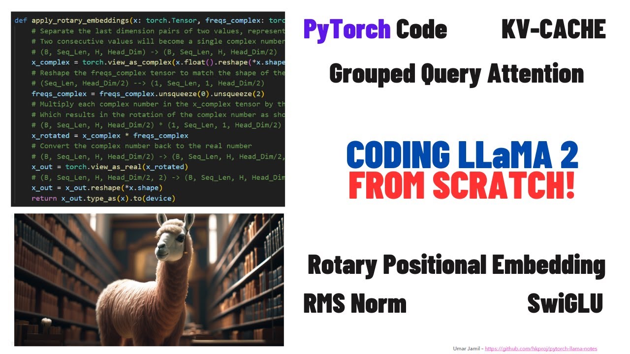
Now let's translate this into code. Apply Rotary Embeddings. X is the token to which we want to apply the Rotary Embeddings. FreqsComplex is the output of this function, but only for the position of this token. So only for all the positions of this token. Because this will have all the theta for all the possible positions, but we only need the positions for this particular token.

And then we need the device. The first thing we do is the transformation number 1, I think I call it. Yeah, this one here. And number 1 and number 2. So the first thing we do is we call the transformation number 1. And number 2. So the first thing we do is we transform the two consecutive dimensions into a new tensor.

And then we visualize it as a complex number. These operations are supported by PyTorch. So we do them. So we create XComplex is equal to. Okay, this operation here is basically saying take two consecutive dimensions and group them. And then we transform this intermediate tensor into a complex tensor by using the view as complex operation from Torch.

Let me write some comments. So we are starting from B, sequence length, H, head dimension. Because I saw before this X is actually not the original vector, but it's already the one divided with its head dimension. Because we will have a multi head attention. But if there is no multi head attention, then this head dimension is actually the full dimension of the token.

So 4096. Then we have this tensor here. But this tensor has two dimensions less than this one. It doesn't have the batch dimension. And it doesn't have the head dimension. So we need to add it. So take the XComplex and we add the two dimensions that it's missing. And here we are doing.

Okay, let me write all the transformations. Here we are going from here to divide by two. Why divide by two? Because every two consecutive pairs are becoming one complex number. And here we go from sequence length to head dimension divide by two. We are mapping it to one because this is the batch dimension sequence length, then the head dimension one, and then head dimension divide by two.

Now we multiply them together. So we do this operation here. So element wise multiplication, which will result in a rotation as we saw in the figure before. So that's why I call it X rotated is equal to X complex multiplied by the complex number of the frequencies. In this case, we are doing sequence length.

H dimension divide by two. Then we multiply it, we obtain this result. And then we first transform it into... We transform the complex number into a tensor in which the first item is the real part of the complex number and then the complex part, the imaginary part, and then we flatten it.

So let's do it. This operation view as real will transform the tensor like this. So it's this transformation here in which we transform the complex number into a tensor of two dimensions. Because that's why you can see this additional dimension here. And then we flatten it. You can just say to flatten it with the shape of the original...

with the original tensor we gave it. So become... And this is how we calculate the embedding. So given a tensor of representing a token or a list of tokens, because we have the batch dimensions, we can apply the embeddings like this doing all these transformations that we have done here and that are represented in this code.

And they are all equivalent to doing this operation as written on the paper. Now we need to go forward with our transformer by implementing the rest. The next thing that we can implement is this RMS norm because it's present at the output of the transformer but also at the input.

So let's go review again the architecture. We can see that we have the normalization, the RMS normalization here but we also have it here and here. So let's implement it. Let's also visualize how the RMS norm works. If you want to have a deep understanding of how normalization works, in my previous video about Llama, I actually described why we need normalization, how it was historically done and how it works, also at the autograd level.

So I will not repeat the same lecture here. I will just briefly introduce how it works. But if you want to have a better understanding, please watch my previous video. So as you remember, in the original transformer, we used layer normalization. And layer normalization worked like this. We have an input where we have some items, suppose item 1, item 2, up to item 10.

Each item has three features, so A1, A2, A3. What we did with layer normalization, we computed two statistics, one for each item, so mu and sigma, so the mean and the sigma. And we standardize each item, normalize each element of this input matrix, using this formula here, which transforms it into a distribution with zero mean and variance of one.

And this formula comes from probability statistics. So as you know, if you have any random variable with its mu and sigma, if you do the variable minus its mean, divided by the standard deviation, so the square root of the variance, it will result into a Gaussian of mean zero and the standard and the variance of one.

We then multiply this with the gamma parameter and we also add a beta parameter here. But this was done in the layer normalization. In LLAMA, we use RMS normalization and let's see the difference. In RMS normalization, the paper of the RMS normalization claims that we don't need to obtain the effect of layer normalization, we don't need to compute two statistics, that is the mean and the variance.

And actually they claim that the normal, the effect given by layer normalization can be obtained without recentering the values. So without recentering them around the mean of zero. But just by scaling. However, the variance in the layer normalization was computed using the mean, because if you remember the formula of the variance is X minus the mean of the distribution to the power of two divided by N.

So to compute the variance, we needed the mean, but we wanted to avoid computing the mean because we don't need it. This is not what the RMS paper claims. RMS paper claims that we don't need the mean and we don't need to recenter. So we need to compute a statistic that doesn't depend on the mean.

That's why they introduced these statistics here, which is the root mean squared that doesn't depend on the mean. And in practice gives the same normalization effect as the layer normalization. And we also have a gamma parameter also here that is learnable and that's multiplied. So as you can see, the only difference between layer normalization and RMS normalization is that we don't recenter the values.

And it looks like that recentering was not necessary as written in the paper, because they say in this paper, we hypothesize that the rescaling invariance is the reason for the success of layer norm rather than the recentering invariance. So they just rescale the values according to the RMS statistic.

And this is what we will do in our code. So let's build this block. (keyboard clicking) So the APS value you can see here is used as a denominator. Let me go back here. It's used here as the added to the denominator. So to avoid a division by zero.

And then we have the gamma parameter. (keyboard clicking) And this is it. Then we define the function norm. (keyboard clicking) Where x is batch sequence length dimension. Okay. So we return x multiplied by torch dot r sqrt. r sqrt stands for the one over the square root. (keyboard clicking) And that's it.

(keyboard clicking) We multiply by gamma. (keyboard clicking) So we have, as you can see, weight is actually is a number, a list of ones with the dimension dim. So dim multiplied by b sequence length dim results in b sequence length dim. Where b is the batch dimension. And here what we are doing is, this is r sqrt is equal to one over sqrt of x, just as a reminder.

And the dimensions here are multiplied by b sequence length one, which results in b sequence length dimensions. So what we are doing is exactly just this formula here. So just multiply it by one over rms and then multiply it with gamma here. Now that we have also built the rms norm, let's go check our next building block, which is this encoder block.

So what is the encoder block? Let's go back to the transformer. Here we have the encoder block is all this block here that contains a normalization. It contains a self-attention here. It contains skip connections. You can see here another normalization, another skip connection and a feed forward layer here.

I think the easiest one to start with is the feed forward, but we can also, we can also, okay, let's start first build the encoder block and then we will build the attention and finally the feed forward. So we first build the skeleton of this, then the attention and then this, let's go.

(keyboard clicking) I received some parameters. (keyboard clicking) What is the head dimension is the dimension of the vector divided by the number of heads. So 4,096 divided by, here is the divide by 32, because as we can see here, we have the dimension of the vector, of the embedding vector is 4,096, but we have 32 heads.

So each head will see 4,096 divided by 32 items from each token. (keyboard clicking) Then we have a self-attention block. I define it, but don't build it right now. Just define the skeleton. Then we have the feed forward. (keyboard clicking) Then we have the normalization before the self-attention. So self-attention, this is our RMS norm.

(keyboard clicking) And this is the motivation behind this argument norm abs. (keyboard clicking) Then we have an after the feed forward. (keyboard clicking) Is it after? It's after the attention, not after the feed forward. (keyboard clicking) So before the feed forward block. (keyboard clicking) And then we have norm abs.

(keyboard clicking) Okay, okay. Now let's implement the forward method. (keyboard clicking) StartPause indicates the position of the token. I kept the same variable number as in the original code. It's actually the position of the token. Because as you remember, we will be dealing with only one token at a time.

So StartPause indicates the position of the token we are dealing with. (keyboard clicking) These are the pre-computed frequencies. (keyboard clicking) So we need to the skip connection. And yeah, okay. The hidden is equal to x plus the attention. So we calculated the attention of what? Of the normalized version of this input.

So we first apply the normalization. (keyboard clicking) And then we calculate this attention. And to the attention, we also give the frequencies. Because as you remember, the rotary positional encodings are kind of, they come into play when we calculate the attention. And these operations involve tensors of size B, sequence length dimension, which is x plus the skip connection, plus the output of the attention, B sequence length dimension, which results in B sequence length dimension.

Then we have another, we have the application of the feedforward with its skip connection. So out is equal to h plus. (keyboard clicking) And before we send it to the feedforward, before we applied the normalization. (keyboard clicking) And this is the output. Now we need to build the self-attention and the feedforward.

Let's start with the harder part first. So the self-attention, because I think it's more interesting. Before we build the self-attention, let's review how self-attention worked in the original transformer and how it will work here. So, okay, this is the original paper from the original paper of the transformer. So attention is all you need.

Let's review the self-attention mechanism in the original transformer. And then we will see how it works in Llama. In the attention is all you need. We have an input, which is sequenced by the model. So a sequence of tokens, each token modeled by a vector of size T model.

We transform them into query key and values, which are the same input. We multiply by a W matrix, which is a parameter matrix, which results in a new matrix, which has this dimension of sequence by D model. And we then split them into the number of heads that we have, such that each vector that represents the token is split into, suppose we have four heads.

So each vector, each head will see a part of the embedding of each token. So if the token was 512 in size, for example, the embedding vector, the first head will watch 128 dimensions of this vector. The second head will watch the next 108 dimensions. The next head will watch the next 108 dimensions, et cetera, et cetera, et cetera.

We then calculate the attention between all these smaller matrices. So Q, K and V. This results in head 1, head 2, head 3 and head 4. We then concatenate them together. We multiply with the W matrix. And this is the output of the multi-head attention. In this case, it's called self-attention because it's the same input that acts as a query, as key and values.

In case the query comes from one place and the key and the values come from another place, in that case, it's called cross-attention. And that kind of attention is used in multi-modal architectures, for example, when you want to combine, for example, pictures with captions or music with text, or you want to translate from one language to another.

So you have kind of multi-modality and you want to connect the two together. But in our case, we are modeling a language. So self-attention is what we need. Actually, attention is all we need. So let's watch how it works in LLAMA. Okay, in LLAMA, we need to talk about a lot of things before we build the self-attention.

We need to review how the self-attention works in LLAMA, how is the key, what is the KV cache, what is the grouped query attention, and actually how the inference works. So we need to review all this stuff before we proceed with the code. Otherwise, it will be very hard to follow the code.

So let's first talk about the inferencing. Given, suppose we have a model, so that has been trained on this particular line. So the line is love that can quickly seize the gentle heart. And this is a line from Dante Alighieri. You can see this from the epistle from the Inferno, Fifth Canto.

It's not the first line actually, but this is Paolo and Francesca, by the way. And we have a model that has been trained on this line, love that can quickly seize the gentle heart. Now, a model that has been trained on this particular line using the next token prediction should have an input that is built in this way.

So the start of sentence, and then the tokens that represented the sentence, then the target should be the same sentence with the end of sentence. Because the transformer is a sequence-to-sequence model, it maps one input sequence into an output sequence of the same size. This means that the first token will be mapped to the first token of the output.

The second token of the input will be mapped to the second token of the output. The third token of the input will be mapped to the third token of the output. But it's not a one-to-one correspondence. Because of the mask, of the causal mask that we apply during the self-attention, to predict this particular token can, for example, the model doesn't only watch the same token in the input, so that, but also watch all the previous tokens.

So the model to predict can needs to access not only that, but also SOS, love, that. And the self-attention mechanism with its causal mask will access all the previous tokens, but not the next ones. This means that when we do the inferencing, we should do it like this. We start with the start of sentence and the model will output the first word.

To output the next token, we need to give the previous output token as input also. So we always append the last token of the output to the input to predict the successive tokens. So for example, to output that, we need to give SOS, love. To output the next token, we take this that and we put it in the input so that we can get the next word.

To output the next token, we need to append the previous output to the input to get the new output quickly. Now, when we do this job, the model is actually, we are giving this input, which is a sequence of four tokens, and the model will produce a sequence of four tokens as output.

But this is not really convenient when we do the inferencing because the model is doing a lot of dot products that are not necessary, that have already been built. For example, what I want to say is that in order to get this last token quickly, we need to access all the previous context here.

But we don't need to output love that can because we don't care. We already have these tokens. We only care about the last one. However, we can't just tell the transformer model to not output the previous tokens. We need to change the calculations in such a way that we only receive at the output of the transformer only one token so that all the other tokens are not even calculated.

And this will make the inferencing fast. And this is the job of the KVCache. Let me show you with some diagrams. As you can see, at every step of the token, we are only interested in the last token output by the model because we already have the previous ones.

However, the model needs to access all the previous tokens to decide which token to output because the model needs to access all the prompt to output the next token. And we do this using the KVCache to reduce the amount of computation. So let's do with some examples. Suppose we do the same job that we did before.

So the inferencing of that model. We give the first token, so the SOS. This will be multiplied. This is the self-attention. So it will be multiplied by the transposed of the keys. This will produce this matrix here, which is one by one. So you can check the dimensions. One by 4,096 multiplied by 4,006 by one will output a matrix that is one by one.

This will be multiplied by the values and this will result in the output token. So this is the inferencing step one in which the only token we give is the start of sentence. Then we take this token output, the token at the output. This is actually not the token because this has to be mapped to the linear layer, etc, etc.

But suppose this is already the token. And we append it to the input. So it becomes the second input of the input. So this is SOS and this is the last output. We multiply it by the transposed of the keys. We get this matrix here. We multiply it by the values and we get two output tokens as output because it's a sequence to sequence model.

Then we append the output of the previous as the input and we multiply it by the transposed of the keys. We get this matrix here. We then multiply it by the Vs and we get three tokens as output. We then append the output of the last one at the Q.

We multiply it by the transposed of the keys. We get this matrix here. We multiply it by the V and we get this sequence as output. But we see some problems. And the one that I told you before. We are doing a lot of computations that we don't need.

First of all, these dot products that we are computing here because this is the self-attention. So Q multiplied by the transposed of the keys will result in a lot of dot products that result in this matrix. These dot products that you see here highlighted in violet have been already computed at the previous steps because we are at the step number four but these have already been computed at the previous step.

Plus, not only they have been computed already, we don't need them because we only are interested in what the latest token that we added as the input, so to the prompt, what is this tokens dot product with all the other tokens because this tokens dot product with all the other tokens will result in the output of the last token, the one we are interested in.

So if there is a way to not do all these computations again and also to not output all the previous tokens that we actually don't need because we always access the latest token, yes, we just use the KVCache. In the KVCache, what we do is we always take the last token and we use it as input.

So we don't append it to the query. We just use it directly as query. But because the query needs to access all the previous tokens, we keep the keys and the values. So we append the last input to the keys and the values but we don't append it to the queries.

We replace it entirely with the queries. Let's see with an example. For example, this is our first step of inferencing. So this is just the start of sentence token. So we just have one token. We multiply it by the transpose of the keys. It will result in one by one.

So we only have one token as output. This token, in the previous case, was appended to the queries. So in the next step, it became a matrix of dimension 2 by 4096. But in our case, at the time step 2, we don't append it. We only append it to the end of the keys and the values.

And we only keep the queries here. If we do this product again now, we will see that this row here is the only one we are interested in. So the one that was not violet in the previous diagram. And if we do this dot product, it will result in only the last token, the one we are interested in.

And every time we keep doing this job, we will see the key and the values grow. The queries will be always the last token. But the number of dot products that we are doing during the inferencing is much less. We don't need to do all those dot products that we did before.

So compare this is time step 4. This is 4 dot products. Compare it with the previous time step 4. So here we have 16 dot products. So we reduce it by a factor of 4. And so that's why it's much faster to do inferencing with the KV cache. And let's review again.

So here, as you can see, the matrix QK. And every time we add the token to the queue grows, right? But all these previous values with the KV cache, we are not computing it again. So that's why this is much faster. We only compute the one we need. And we only get one token as output.

If this mechanism is not clear, please watch my previous video about LAMA, in which I describe it in much more detail and also with much more visualizations. Now let's go build this. There is another thing actually I want to show you before we go to build it, which is the grouped query attention.

This one here. So I call it grouped multi-query attention, because it's actually the successive version of the multi-query attention. It's something in between the multi-head attention and the multi-query attention. But actually, the real name is grouped query attention in the paper. Also, it's called grouped query attention. Now, the reason we introduced the grouped query attention is first of all, we had the multi-query attention.

The multi-query attention basically were introduced to solve one problem. That is, we first had the multi-head attention. We introduced the KV cache with the multi-head attention. Just the one we just saw. The problem was that with the multi-head attention, we were doing too many dot products. With the multi-head with the KV cache, we do less dot products.

This resulted in a lot less computation. But it also resulted in a new bottleneck for the algorithm. So the bottleneck was not longer the number of computations, but how many memory access we were performing to access these tensors. Because in the GPU, the GPU is much faster at doing computations than it is at moving tensors around in its memory.

So when we optimize an algorithm, we not only need to consider how many operations we are doing, but also how many tensors we are accessing, and where are these tensors located. So it's not a good idea to keep copying tensor from one place to another, because the GPU is much slower at copying memory from one place to another than it is at computing operations.

And this can be visualized on the datasheet of the GPU. You can see, for example, that computing operations is 19.5 Tera floating point operations per second. And while the memory bandwidth, so how fast it can move memory, is 40 times slower. So we need to optimize algorithms also for managing how many tensors we access and how we move them around the memory.

This is why we introduced the multi-query attention. The multi-query attention basically means that we have many heads for the queries, but we only have one head for the key and the values. This resulted in a new algorithm that was much more efficient than the algorithm just with the KVCache.

Because the KVCache, yeah, it reduced the number of dot products, but it had a new bottleneck, that is the number of memory access. With this algorithm, we also may optimize the memory access, but we lose some quality, because we are reducing the number of heads for the key and the values.

So we are reducing the number of parameters in the model. And this way, the model, because we are reducing the number of parameters involved in the attention mechanism, of course the model will degrade in quality. But we saw that practically it degraded the quality not so much. So actually the quality was not bad.

And this was in this paper. So they show that the quality degradation was very little, so from 26.7 to 26.5, but the performance gains were very important. We went from 48 microseconds per token to 5 microseconds or 6 microseconds per token, so a lot faster. Now, let's introduce the grouped query attention or the grouped multi-query attention.

In the multi-head attention, we had n heads for the queries, n heads for the keys and n heads for the values. In the multi-query attention, we have n heads for the keys, but only one head for the keys and the values. In the grouped multi-query attention or the grouped query attention, we have less number of heads for the keys and values.

So every two heads for the queries, in this case, for example, we will have one head for the keys and the values. And this is a good balance between quality and speeds, because, of course, the fastest one is this one, because you have less heads. But, of course, the best one from a quality point of view is this one, but this is a good compromise between the two.

So you don't lose quality, but at the same time, you also optimize the speed compared to the multi-head attention. So now that we have reviewed all this concept, let's go build it. So please, again, if you didn't understand very much in detail, this part is better. You go to review my other video about Llama, in which I explain all this part much better.

Otherwise, if I have to repeat the same content of the previous video, this would be the current video would become 10 hours. So let's go build it. Okay, we need to save some things. Compared to the original code from Facebook, from Meta, I actually removed the parallelization. First of all, because I cannot test it.

I don't have multiple GPUs. I don't have a very powerful GPU, actually. And so I simplified the code a lot. And KVHeads indicates the number of heads for the keys and the values, because they can be different than the number of heads for the queries. And this is why we also have an headsQueue.

This value here represents the ratio between the number of heads for the query and the number of heads for the keys and the values. We will use it later when we calculate the attention. So let me write some comments. So this is… So… And then we have a self.headDimension, which is… Which is… This indicates the part of the embedding that will be visualized by each head.

Because, as you know, the embedding is split into multiple heads. So each head will watch the full sentence, but a part of the embedding of each word. Then we have the W matrices. WQ, WK, WV, and WO, just like in the normal vanilla transformer. And they don't have any bias.

Oops, why did I write true? And then we create a cache. We will see later how it's used. I just now created one for the keys and one for the values. So… Okay, finally, we implement the forward method, which is the salient part here. So, self x is… To simplify the code for you, I will write the… For each operation, I will write the dimensions of the tensor that is involved in the operation, and also the resulting tensor from each operation.

The start position indicates just the position of the token inside of the sentence. And these are the frequencies that we have computed. Okay, let's start by extracting pipe size. B, sequence length, and dimension. But the sequence length, we know it's one. So, dimension, yeah. Then what we do is we multiply, just like in the original transformer, we take the query, the key, and values.

We multiply it by then the WQ, WK, and WK matrix. So, xq is equal to self.wq. This means going from B, one dimension, to B, one head dimension. So, the number of heads for the query multiplied by the dimension, because we are… In this case, we are… This is actually equal to dim.

So, the number of heads multiply the head dimension, as you can see from here. So, we are not changing the shape. In this case, however, we may change the shape of the… Because the number of heads for the kv may be smaller than q. So, this matrix may have a last dimension that is smaller than xq.

And the same is for xv. So, here, let me write some comment. Apply the WQ, WK, and WV matrix to queries, keys, and values, which are the same, because it's a self-attention. So, the query, key, and value is always x. We then divide them into their corresponding number of heads.

So, xq is equal to xq.q. Batch size, we keep it like this. Sequence length is one. So, we divide b1, h, q multiplied by head dimension into b1, head, h, q, and head dimension. So, we divide them into the h heads for the query. And then we do the same for the key and the values.

And the same for the b. So, so, now, we have multiplied, okay, we have the x input, we multiply it by the WQ, WK, and WK, y. Let's go check the code here. As you remember, we take the input, we multiply it by WQ, WK, and WV. This will result in these matrices here.

We then divide them into the number of heads. But in the case of grouped query attention, they may be different. So, this may be four heads, and this may be two heads, and this may be two heads. So, they are not the same number. The next thing we are going to do, and this is present in the here, we need to apply the rotary positional encodings to the query and the keys, but not the values.

Let's do it. And this is how we apply the positional encodings. This will not change the size of the vectors. You can see that here. Because at the end, we have the same shape as the original input vector. Okay. Now, now comes the KVCache part. Let's watch again the slides.

As we can see here, every time we have an input-output token, so for example, the attention 2 here, it supposes the token number 2, we append it at the end of the keys and the values. And this is exactly what we are going to do. So, what we do here, we keep a cache of the keys and the values, because they will be used for the next iterations.

Because at every iteration, in X, we only receive the latest token that was output from the previous iteration. We append it to the K and the V, and then we compute the attention between all the K, all the V, but only the single token as query. So, let's do it.

So, first, replace. This is the position of the token. This should be 1, because sequence length is actually 1, always. But I try to keep this code the same as the one from Lama, from Meta. This is, basically, it means that if we have one token from many batches, I mean, we have one token for every batch, we replace them, because we can process multiple batches.

So, we replace the entry for this particular position for every batch. Okay. Now, we replace it only for this position here. But when we compute the attention using the KVCache, let's go watch again, we need to calculate the dot product between the only one token but all the keys.

And then we will need to multiply with all the values, and this will result in only one token as output. So, we need to extract from this cache all the tokens as keys and all the tokens as values up to this position here. The one we are passing. So, keys is equal to all.

So, starting from 0 up to startPos plus sequenceLength, and the values are length. Now, what happens is that, let me write also some sizes here. We have b, sequenceLength of K and V, because the sequenceLength of the input is always 1, we know that. But the sequenceLength of the cache means all the cached keys and values, which are up to startPosition.

So, this sequenceLength is actually equal to startPosition. And actually, startPosition plus 1. My next dimension is the number of heads for the K and V, and then the dimension of each head. Now, the number of heads for the keys and values may not correspond to the number of heads of the queries.

So, how do we compute? In the original code from Lama, what they did was basically, let's go check the code for here. So, in the grouped query, attention, we have that the number of heads for the keys and the values is not the same as the number of heads for the queries.

So, there are two ways. One is to make an optimized algorithm that actually takes this into consideration. The other way is to just copy this single head into multiple heads, such that we arrive to this situation here, and then we just compute it just like a multi-head. This is not an optimized solution, but it's the one used by the code by Lama.

And it's also the one I will be sticking to, because I don't have any way of testing other codes, because the only model that supports the grouped query attention is the biggest one from Lama, so with 70 billion parameters, but my computer will never be able to load that model.

And so, I don't have any way of testing it, so that's why I also didn't optimize the code for actually computing the grouped query attention, but I will just replicate this single head multiple times, such that we arrive to this situation here. So, I will also repeat. So, okay, this function here, repeat_kv, just repeats the keys until we reach the number of, for this number of times, so nrep.

What is this? It's the ratio of the number of heads of the queries by the number of heads of the keys. So, if the number of heads of the keys is four, and the number of heads for the queries is eight, that means we need to repeat twice each head.

So, let's build also this method, since we are here. So, okay, we don't need to repeat it, so there is only one repetition. We just return the basic tensor. Otherwise, we repeat it n times. So, the first thing we do is we add a new dimension, and we can do like this, part_sequence_length, number_of_heads, then nothing, and then this will add this new dimension in this position.

Then we expand it. And then we reshape it. Basically, we introduce a new dimension. We repeat all the sequence this dimension number of times, along this dimension n-wrap number of times, and then we just flatten it. So, we remove again this dimension. And this is how we repeat the keys and also the values.

Now we can repeat. Okay, now we just proceed just like with the standard, the standard calculation for the multi-head attention. That is, we first move the head dimension before the sequence dimension, because each head will watch all the sequence, but a part of the embedding of each token. So, what we are doing is batch 1, because 1 is the sequence length of the queries, the number of heads of the queries, and head dimension, batch head sequence length and head dimension.

We do the same for the keys and the values. Then we do the standard formula for queries multiplied by the transpose of the keys, divided by the square root of the dimension of each head. So, xq, so the queries multiplied by the transpose of the keys, all of this divided by the square root of the dimension of each head.

Then we apply the softmax, and this one will result in a shape of queries, one head dimension multiplied by qv. The softmax doesn't change the dimension. Then we multiply it by the values. So, the formula is queries multiplied by the transpose of the keys, and then we do the softmax, then the output is multiplied by the values.

So, this will result in b, and then we multiply it by the output matrix, but before we remove all the heads, so we concatenate again. This is what we did also here. So, here we take the output of all the heads, then we concatenate them together, and then we multiply it by the wo matrix.

So, and this will result in a b1 dim, b1 dim, this one is bhq one head dimension into b1 hq head dimension, because of the transposition, and then we remove the dimension for the head, so b1 dimension. And this is our self-attention with kvcache. So, let's review what we have done.

Here, I think I made some mistake, because self, that's why it's colored differently. Okay, let's review what we have done. When we calculated the self-attention, because we are inferencing, so this code will only work for inferencing, we can use the kvcache. The kvcache allow us to save a number of dot products that we don't need.

Why? Because every time we are in the original transformer, we were computing a lot of dot products for tokens, output tokens that we don't care about. In this case, we simplified the mechanism to output only one token. As you can see, the output of the self-attention is b, so batch, one token only with its embedding size, which is 4096.

So, we are only outputting one token, not many tokens. We input only one token, and we output one token. But because we need to relate that single token with all the previous tokens, we keep a cache of the keys and the values. Every time we have a token, we put it into the cache, like here, then we retrieve all the previous saved tokens from the cache, and then we calculate the attention between all the previous tokens, so the keys and the values, and the single token as input of, as queries.

The output is the only token we care about. This is the idea behind kvcache. And the grouped query attention is the fact that we have a different number of heads for the keys and values, but in our case, we do have a different number of heads for the keys and queries.

But we just repeat the one that we are missing to calculate the attention. So the attention is calculated just like the previous transformer, like a normal multi-head attention, but by repeating the missing keys and values heads, instead of actually optimizing the algorithm. This has also been done by Meta in its official implementation, and I also did it here.

The biggest reason is because I cannot test any other modification. I cannot test another algorithm that actually tries to optimize this calculation. So if I find another implementation that I know is working, I will share it with you guys. Otherwise, I will try to run it on Colab and see if I can come up with a better solution.

But for now, we just repeat it. But at least we got the concept of the grouped query attention. That is, we have less number of heads, and it's something that is in between the multi-query attention and the multi-head attention. That doesn't sacrifice quality, but improves speed. Now, the last thing that we didn't implement is the feedforward layer.

For the feedforward layer, the only thing that we need to review is the ZWIGGLU activation function that we can see here. And this activation function has been changed compared to the previous activation function used in the vanilla transformer, which was the RELU function. And the only reason we replaced it is because this one performs better.

And as I showed in my previous video, we cannot prove why it works better. Because in such a big model with 70 billion parameters, it's difficult to explain why a little modification works better than another. We just know that some things work better in practice for that kind of model or for that kind of application.

And this is actually not my opinion. This is actually written in the paper. So as you can see here in the conclusion of the paper, they say that we offer no explanation as to why this architecture seems to work. We attribute their success as all else to divine benevolence.

So it means that when you have such a big model and you change a little thing and it works better, you cannot always come up with a pattern to describe why it is working better. You just take it for granted that it works better and you use it because it works better in practice.

So to implement the ZWIGGLU function, we need to apply... This is the formula from the original transformer. So we have two matrices here. So this is the RELU function of the first linear layer and the second linear layer. In LAMA, we use the ZWIGGLU function which involves the three matrices here.

Because they incremented the number of parameters here and also they were experimenting with the grouped query attention, the architecture of LAMA has some more parameters to adjust the number of parameters of this feedforward layer. So as it respects some constraints. And this is actually used in deep learning research.

Whenever we modify the transformer model and this reduces the number of parameters or increases the number of parameters, the first thing the researchers do, they adjust the numbers of parameters of the feedforward layer so that when they make comparison between two models, they have the same number of parameters.

So I will also, of course, use the same structure because otherwise I cannot load the weight from the pre-trained model. So let's do it. The hidden size is calculated like this. So four times the dimension. Then they do the two-third of this dimension. And then they also have a multiplier if it's specified.

Then they say round the hidden... oops. By using this modification to calculating the hidden dimension like this, it may not be the case that this hidden dimension is a multiple of this number here. So maybe they want the size of the hidden dimension to be multiple of this number here.

So maybe they want the size of the hidden dimension to be multiple of this number here. So maybe they want the size of the hidden dimension to be multiple of this number here. So maybe they want the size of the hidden dimension to be multiple of this number here.

So maybe they want the size of the hidden dimension to be multiple of this number here. So maybe they want the size of the hidden layer to be a multiple of 256. But by calculating it like this, it may not be. So what they do is they make it round up to the next multiple of the multiple of parameter.

So this is a way to do it. Okay, let me give you an example. It's easier to show with an example than to actually write it. So suppose you have the hidden size is equal to, let's say, 7. But you want it to multiple of is equal to 5.

So you want the hidden size to be a multiple of 5. So how do we do? Well, what we do is, basically, we do hidden plus 4 in this case. So we do 7 plus 4, which is 11. We divide it by 5, which is equal to 2. And then we multiply this 2 by 5.

So it will result in 2 by 5 is equal to 10. It will result in the first multiple that is bigger or equal to this number here. That's the idea. And then we have these matrices for the Zwiglu function. It's very easy. We just follow the formula for the Zwiglu function, which is here.

So w, the Zwish of, what is Zwish? The Zwish is the Sillu function. Because the Zwish with the beta is equal to 1 is actually the Sillu function, which has this graph here. And then we multiply it with another parameter matrix here. And then we apply it to another linear layer, w2.

So in total, we have three matrices, w1, we call it w2, and w3. And they don't have bias. Oops. This is the hidden dimension. Okay, now we implement the forward method. The first thing we do is we calculate the Zwish function. Then we calculate, so we are calculating, let me show you.

We are calculating this one, xw, Zwish of xw. Then we calculate this xv. Then we multiply them together, just like in the formula. So Zwish multiplied by xv. And then we apply the last linear layer, which is w2. Which results in a multiplication by the w2 matrix, by the way.

And then we return x. And this is the field forward layer. Now that we have all the building blocks, we need to go to the inferencing. Let's start building the inference code. So inference.py, the first code we will be, first we will build a code to load the model.

And then we will build a code to inference the model. I will actually also show all the inference techniques that are out there, and which one we will apply and why. So let's start by building first the code for loading the model. So first we import the stuff we need.

We need the JSON to load the parameters. And then we need the sentence piece to load the tokenizer. Because the sentence piece is the tokenizer that has been used, and it's a library from Google. Okay. From model import model-args and the transformer class. We define the class Lama, which is our model.

It takes a transformer, a tokenizer, which is a sentence piece processor. And then the model arguments. Oops. Oops. Args. Model-args. Yeah. Model-args. Okay. Now we build a static method. Static method. And we call it build, just like in the original code from Lama. In which we pass the directory where the checkpoints are saved.

In this case, the directory name is lama27b, in my case. But it depends on which size of the model you have downloaded. Then the tokenizer path, which is the path to the tokenizer. This is the file of the tokenizer that I downloaded. Then we have a load model layer, max sequence length.

Max patch size. And we have device. Okay. This is only for displaying how much time it takes to load the model. If we want to load the model, we will also load the checkpoints. So checkpoints is equal to sorted. The glob method allows you to find all the files that match this filter.

Okay, we see that we are loading checkpoint this one. And then we actually load it. And we save it on the CPU. We can show how much time it takes to load the model. In my computer, usually it takes 10 to 20 seconds. Then previous time we rewrite it.

So we can also show how much time it takes to load all the parameters of the model. Then we load the parameters, so the JSON file. We read it, open it as read-only file. And okay, then we build the arguments. Maximum sequence length is the one we have specified.

And then we have the max patch size is the max patch size. The device is the one we have specified. And then all the parameters loaded from the JSON file. Then we loaded the tokenizer. Then we, by using the tokenizer, we can populate the vocab size of the model args.

The vocabulary size is actually the number of tokens inside the tokenizer. Now this is also the default tensor for PyTorch. So whenever PyTorch wants to create a new tensor, what kind of type it should use, it's defined, this is by meta, so they want for CUDA to use this type that I show you here.

Default tensor type torch.cuda half tensor. This changes the precision that the tensor supports. So how much space it occupies in memory. Otherwise, then we created the actual model. Okay, when we load a checkpoint, actually the checkpoint is a list of key and values. Each key is a matrix in the model.

So the weight, for example, of a linear layer, or the bias of a linear layer, or something like this. And the names that we have used for the variable names and the matrices here, for example, wqwk, match actually the name that are present in the checkpoint here, except for one name.

So to make sure that I have used the right names, I will load the checkpoint with strict equal true. Strict equal true means that if there is at least one name that doesn't match, it will throw an error. So if load model, model.loadState ticked, strict equal true. So if there is at least one name in the loaded file that doesn't match the name in the classes that I have created here in the model, it will throw an error.

But I know that there is one key that we don't need, which are the frequencies for the rotary positional embeddings, which we actually are computing every time we create the tensor. So we are creating them here by using this function. So we don't need to load them from the model.

So we can remove it from the model, from the checkpoint. So because the checkpoint is a dictionary, we can just remove this. It's called rope.freqs. And then we can print how much time it took to load the model. And then we return llama. Model tokenizer. And model args. Now, before we proceed further, let me test if the model can be successfully loaded.

So let's do it. If name... First, I will set the manual seed to zero. So later we use it for inferencing. Then I don't want to use CUDA because my GPU doesn't support it. So I say allow_cuda = 4. Then device is equal to storage.cuda.is_available and allow_cuda else cpu.

Next time if you want to load the model with CUDA, just set this variable to true. But in my case, I will always leave it to false because I don't want to load CUDA. Sequence length, I set it to 1024. Max batch size, let's say 3. And device now.

Let's run it and hopefully it will not crash. Wow, already. Not tensore, but tensor. So let's run it again. There is always a lot of typos when you write code. Another problem here. Ah, not storage, but tensor. This should be tensor. bfloat16 tensor. Yeah, let's try again. Hidden... hidden what?

Hidden dimension, of course. And let's try again. Yeah, all okay. Okay, wonderful. It means that at least it's doing something and it's not crashing, which is always a good news. So let's run it again. Okay, wonderful. It means that at least it's doing something and it's not crashing, which is always a good news.

So our next step is actually to build the inferencing code. So what we want to do is actually we want to be able to give some prompts to the model and then check the output for this prompt. So let's define some prompts. We will define some prompts here. And here we pass, for example, the size of the prompts.

And then we want to, you know, we want to inference the model. So before we start inferencing the model, we need to build the code for inferencing the model, because we need to find a strategy for selecting the next token, etc, etc. So let's review how the inferencing works and what are the various strategies for inferencing.

Okay, so when we are dealing with the next token prediction task, when we want to inference, we usually give the prompt and then we want to predict the tokens. But we give one token at a time. And every time we give one more token, the model will output one more token as output.

And we only keep the last one. But with the KVCache, actually, we always give one token at a time. The KVCache will keep the cache for the keys and the values and with only output one token. Okay, the point is, we need to find strategies for selecting this token.

Among all the tokens that we have in the vocabulary. And this is the job of the logits and the softmax. So let's review how they work. Now imagine I give you the following task as human. So complete the following sentence. I think nuclear power is and then you have to choose a word.

Now you as human may have thought of the possible next tokens, which may be clean, dangerous, cheap, expensive, safe, difficult, or something else. The choice of the next token in your head depends on your education, on your experience with nuclear power, and your opinion on the matter. Large language models also face the same problem.

When we give them a prompt, then the model has to choose the next word. The model, the uncertainty of the choice derives entirely from their training process and the strategy that we use to select the next token. There are many strategies. For example, we have the greedy strategy, the beam search, temperature is a parameter, random sampling, top k, top p.

In this video, we will review all these strategies and how they work. But first, we need to understand what are the logits. Let's look at the transformer model from Lama. So the output of the self-attention is a sequence. In the case of the KVCache is only one token. We then run it through a linear layer.

So after normalization, we run it through a linear layer. The linear layer will transform the embedding that is output from the self-attention here into a list of numbers that represent the kind of the probability, they are not really a probability, but we can think of it as a probability, of that token in the vocabulary.

So if our vocabulary is made of, let's say, 100 tokens, this linear layer will output 100 numbers. And after we apply the softmax, these 100 numbers will become the probability of that token being the next more probable token for the prompt given to the input. So given an input, a prompt, the model comes up with probabilities.

Probabilities for which token to choose next. And so what is the job of the linear layer and what is the job of the softmax? The linear layer converts the embedding of a token into a list of numbers such that each number represents a score that later with the softmax represents the probability of that particular token in the vocabulary.

The softmax job is just to scale the logits in such a way that they sum up to one. So that's why we can talk about probabilities with the softmax, but not with the logits. So the output of the softmax is thus a probability distribution over all the words in the vocabulary.

That is, each word in the vocabulary will have a probability associated with it. But now, given these words, each one with their probability, how do we choose the next token? There are many strategies. The easiest one is the greedy. The greedy strategy basically says we just select the token with the maximum probability.

So imagine we are inferencing and the time step is the first time step in the greedy strategy. The prompt is Celia, you're breaking my heart. You're shaking my. OK, this is a line from a very famous song from Simone Ergampfunkel. And the next word, for those who know, will be confidence.

So Celia, you're breaking my heart. You are shaking my confidence. Suppose the output of the softmax is this distribution here. So we have 40% probability for this word. 20% for this word. 15% for this word. And 10% for this word. With a greedy strategy, we always choose the token with the maximum probability.

Then we append it to the input. So the input at the next inference step becomes Celia, you're breaking my heart. You're shaking my confidence. And then the model has to come up with the next word, which, if you know the song, is daily. If we use the greedy strategy, we select the one with the highest probability.

So in this case, it's daily, and it's also the correct one. So this is how the greedy strategy works. At every step, we choose the token with the maximum probability, which is then appended to the input to generate the next token, and so on. But if the initial token happens to be the wrong one, so not only the initial, but the initial two, three tokens happen to be the wrong ones, it's very likely that all the next tokens will also be wrong, because we are giving a wrong prompt to the model.

So imagine at the time step one, we don't choose confidence, but somehow the model came up with a high score for liver. So you're shaking my liver, but then the next word, the model will not be able to come up with a reasonable next word, because there is no song that says you're shaking my liver.

So if we make a mistake in the early stage of the greedy, all the next token very probably will also be wrong. But it's very easy to implement. And however, it performs poorly in practice, that it's very, it's not used so much. Another strategy is the BeamSearch. In BeamSearch, we have a parameter, which is called K, which means that at every step, we not only choose the top ones, but the top K at every step.

And we always keep the top two best performing tokens. So in this case, for example, imagine we are time step one. So Celia, you're breaking my heart. You are shaking mine. And the top two words are pizza and confidence. Pizza somehow has a higher, has a higher probability, because maybe the model has never seen this song before.

So it doesn't know that the next word is confidence. So maybe the model outputs these probabilities. But we choose the two top most, the two tokens with the highest probabilities. At the next time step, we make two prompts, one in case we choose the first one, so the first token, and one in case we choose the second token.

And then we see what are the next possible choices if we use the first token. And what are the next choices if we use the second token? So we check the model output for the first prompt and for the second prompt. And in case we use, for example, the first prompt, the model will output these probabilities.

And if we use the second prompt, the model will output these probabilities. What we do then is we calculate the cumulative score for each possible path. So for pizza, for example, the probability was 40%. But after pizza, the model produced the probability for the margarita, for example, is 0.01%.

So for this path, pizza, margarita, it's 0.004. The probability is 0.4%. Pizza, anchovies, it's going to be 0.2% or 0.002. However, with confidence, we get a new next token that can be either daily or monthly. With daily, we get a cumulative score of 0.16 and with monthly of 0.02.

So as we can see, at the time step two, even if at the time step one, pizza was the most probable word, because we kept the second choice alive, so we didn't kill it, just like we did it with greedy. Let me use the laser. We can see that the confidence then produces a next token that is very probable, because now the model has more prompt.

And so it can come up with more specific choices for the next tokens with a very high confidence. So we compute the cumulative score of all these paths, and we keep the two paths that have the top choices. So now the pizza path has been killed, because it's later we chose pizza at the beginning, because somehow the model thought it was pizza, but then it couldn't find it.

The model was not so confident about the next words. But in the case of this token here, the model was very confident about the second score. So we killed all this path here, and we kept this one until we arrived to the last token, in which we just selected the path with the highest score, and that's the output of our inferencing strategy with BeamSearch.

And repeat the steps of the last slide for all the successive tokens until we arrive to the last one. And with BeamSearch, at every step we keep alive the top k paths, and all the others are killed. It increases inferencing time, because at every step we must explore k possible options, but generally it performs better than the greedy strategy, for the reason that I have just shown.

Another thing that is interesting in inferencing is the temperature, because the idea of the temperature is that we can make the model more confident or less confident. So for example, when we compute the logits, which are not the probabilities, so they are what will become the probabilities after we apply the Softmax.

So before we apply the Softmax, we can scale the logits, so that if we use, for example, like this. So for example, we have these logits here. I choose the negative numbers, so the Softmax probabilities are reasonable numbers. And so these are the logits. And if we divide these logits before applying the Softmax by a number that is low, so low temperature, it's called, this number is called the temperature, it will make the model more confident, because it will make bigger probabilities bigger and smaller probabilities smaller.

So the gap between the low and high probability increases. So for example, you can see that without applying any temperature, the highest logit gets 80% probability. But applying a 0.4 temperature, the highest logit becomes 98% probability. And if we apply a high temperature, it makes the model less confident.

So the gap between the low and high probability reduces. The temperature is important if we want to increase the confidence of the model or not, because it can be used in conjunction with other strategies, like, for example, the greedy, or the top k or the top v that we will see later.

Another strategy is the random sampling. So as we saw, the logits are not a probability distribution, but after we apply the softmax, they become a distribution. So what we do, because it's a distribution, we can also sample from this distribution. For example, in this distribution here, that comes from these logits here, we have one token that can be chosen with a 12% probability, one can be chosen with 7% probability, and one that can be chosen with 80% probability.

If we flip a coin, by 80% of the time, we will choose this token, and 12% of the time we will choose this token, and 7% of the time we will choose this token. So this means sample from this distribution. It means take a number from this distribution, according to its weight, to its probability.

Now, there is a problem with this sampling strategy here, that with very little probability, it may happen that we choose tokens that are total crap. For example, in this scenario here, for example, before, with the greedy strategy, or with Bream search, for example, this token here, if we use a random sampling, we will choose the word pizza with 40% probability, the word confidence with 20% probability, but with a very little probability, it may happen that we will choose the word Pokemon with 10% probability.

Of course, the probability is low, so the probability of us making a bad choice is low, but there is this probability. So this is a problem with random sampling. The next strategy is TopKey. In TopKey, what we do is, to avoid selecting the crappy tokens, we just remove them.

So we take all the logits, we sort them, and then we just keep the highest key, so that the crappy one, we just remove them from this distribution, and then we calculate the distribution for the rest. So we apply the softmax only to the ones that survive. The problem is also here.

Given the following, these two distributions, the low probability tokens can still make their way into the TopKey, because it all depends on the distribution to which we apply the TopKey. Let me give you a graphical example. Imagine we have a distribution that is very flat. Suppose this distribution here, so some words, this is our vocabulary.

This is the probability of each word. So the word number one, word number two, word number three, word number four, et cetera, et cetera, et cetera. But more or less, all the words have the same probability. So imagine we take the top 10 words, so it will select all these tokens, right?

Okay. So it will select the token number one, token number two, token number three, token number four, up to whatever token here is here. Imagine we have another distribution that is made like this. So we still have a vocabulary. Vocabulary. We still have a probability distribution. And the distribution is made like this.

So because it's sorted, we have a distribution that is very skewed. Because we still keep the top 10, as you can see, we will select this token, this token, this token, this token, this token. But these tokens here are very crappy compared to this one here. So they will still make their way into our selection.

And this is not something that we want. We want to avoid selecting crappy tokens, but we still want to have some randomness. So we don't want to be totally greedy because sometimes the tokens that are in the top N tokens, maybe they are all reasonable. Also, sometimes the prompt can be quite ambiguous.

So we don't know which, even as humans, we may not know what is the next word to be chosen. So we want some randomness, but we also don't want the very low probability tokens. But with this top case strategy, the low probability tokens can still make their way into our selection.

And this problem is solved with top P. With top P, we only keep the tokens with the highest probability, such that the cumulative probability is greater than or equal to the parameter P. What does this mean? It means that if we have the previous distributions, so one that is quite flat, for example, and the one that has a mode, so for example, this one.

So this one is nearly 90% and the other one are 0.000%, but this more or less all of them are like 0.2% and then they go down. In the case, imagine P is equal to, let's say, 0.5. In this case, we will select all the tokens such that the area under the curve is equal to 0.5.

But here, because this first token is already 0.9, we will actually only select one token and all the crappy ones will not be selected because this area under the curve is already 0.9. And this is the idea behind the top P. So when the model, when the distribution is more flat, we select more tokens because it means that we are more uncertain about which token to choose.

But when we have a big mode, we select fewer tokens and this way we avoid getting the low probability ones. So now that we reviewed all the strategies for selecting the token, we will implement it. And in the case of Lama, also in the official code, they actually implement the top P strategy.

In my case, I think that the BeamSearch is a reasonable choice. So in another video, maybe I will make how to implement the BeamSearch. But for now, I will implement the top P. So let's go build it. So we implement the method, let's call it TextCompilation, which is the same name that's used in the original code from Lama.

Given prompts a temperature that is 0.6. And so 0.6 means that we want to make the model more confident. Top P means that we want all the tokens such that their cumulative probability is at least 0.9. So 90%. Okay, I think here should be lowercase. Okay, so if we didn't specify the max generation length, then we just generate the maximum token.

Args. Just generate as much token as we can up to the sequence length. And then we, first of all, convert each token of the prompt. So each prompt, actually, into tokens using the tokenizer. Mm-hmm. Then, as we saw before, we need to add the beginning of sentence when we pass the input to the model for inferencing.

Mm-hmm. But not the end of sentence. Okay. Because we specified the max batch also for the model when we built it for the KVCache, so we need to make sure that the batch size of the prompts is not too large. Mm-hmm. And then max prompt length is the maximum prompt length that we have in the prompt.

Mm-hmm. I'm not writing any message, even if you should, but okay, for us it's just basically debugging. Then the total length is how many tokens we want to get from the model. Mm-hmm. Okay, now we create the list that will contain the generated token. So, so, this means create a tensor of shape batch size by total length, in which each item is actually the padding token.

And then we fill the initial tokens with the prompt tokens. Mm-hmm. Okay, we also need this variable that tells if we reach the end of sentence in any of the prompts. This indicates if the token in this position is a padding token or not, so true. If the token is a prompt token, false, otherwise.

And then we can finally make the for loop to generate the tokens. DamageRTQDM, range from one. Okay, now we generate one token at a time. So, the logits come from the model, so set.model.forward. We need to pass one token at a time. So, which token? The one currently we want to output.

So, current minus one. Pause. So, only one token. And we also tell the model what is the position of this token, because for the KVCache. And if we use the temperature, we apply it. As you can see, every time when we want to inference, we always select the last token.

But because we are using the KVCache, actually our model will only output one token at a time. So, the next token will be selected according to our topP strategy. So, we have the probabilities. Now we apply the topP. I just define it here. So, sample topP, and then we implement it.

If we didn't specify any temperature, we just use the greedy. So, so okay. Now we have the next token according to this strategy or this greedy. Then we only replace the token if it is a padding token. So, the problem is, we already have some tokens that come from the prompt.

But we don't want to, but we still need to give the prompt to the model. But we are only giving one token at a time to the model to build the initial cache. So, we will give, the first prompt tokens will be given to the model, not because we care about what the model will output for those tokens.

But only because we want the KV cache to be built for those positions. And after we give the last token of the prompt, then we care about what is the model outputting. So, only replace the next token if it is a padding token. And which one is a padding token?

The one that was not an initial prompt token. Because here we build tokens full of paddings. But then, we replace the prompt tokens, the padding tokens with the prompt tokens for the one with the initial tokens. All the others have to be inferred by the model. So, token... This means, basically, check this mask.

What is this mask? If it's true, if the token is a prompt token. So, if it is a prompt token, replace it with this one. And if it's not a prompt token, just keep it the current one. Okay, then... Since we do not care about what the model outputs for the initial prompt tokens, but only for the last prompt token, we don't care if we find an end-of-sentence position for those tokens.

So, end-of-sentence is only reached if we find it for one of the tokens that we actually want to inference, not the one that we send to the model just to build a KV cache. So, okay, this basically means the end-of-sentence for a particular prompt is reached only if it was a padding token.

So, only if it was a padding token. So, it was not a prompt token. This means not. And we actually found an end-of-sentence token from the model output. If all of the prompts have reached the end-of-sentence token, then we stop this for loop. We don't need to inference anymore.

Now, we prepare the output. So, so, so, so, this means that if we found an end-of-sentence token for one of the prompts, we just cut the prompt output there. The model output at that particular token. We don't care about what it outputs next. This is the output text and then we output the tokens and the text.

Hopefully, I didn't make too many typos and mistakes. So, now we need to build the sample_top_p. So, we have the logits that are the output of the model. We transform them into probabilities by using the softmax. But given these probabilities, we need to use the sample_top_p strategy to select all the tokens such that their cumulative probability is equal to top_p, which in our case is 0.9, so 90 percent.

Okay, the first thing we do is we sort these probabilities in descending order. So, we then calculate the cumulative sum. Then we create the mask that says which tokens we want to keep and which one we don't want to keep. So, mask is equal to probability_sum minus probability_sort more than p.

Why do we do a minus probability_sort? Because we want to shift. Let me show you on the slides here. You can see here, for example, the cumulative probability. So, the probabilities are this one, 44 percent, 40 percent, 6 percent, 4 percent, and 3 percent. Then we calculated the cumulative.

That means up to here it's 44 percent. Then this one plus this one is 85 percent. Then this one plus this one plus this one is 91 percent. This one plus this one plus this one plus this one is 96 percent, etc, etc. But imagine we have a 0.90 percent probability or 0.5 percent probability.

We need to keep up to this token here because this one is not enough. It's zero point. So, we need to up to this one. So, the first number that is less than or equal to p. And it's this in case it's this one. So, that's why we shift it.

We want also this token inclusive. And this is why we do this minus probability sort. So, all the ones that we didn't select, we zero them out. Zero. And then we redistribute the probabilities because, of course, if we remove some items from here, they don't sum up to one anymore.

So, we need to redistribute the probabilities. And this is very easy. Okay, then the next token is basically, suppose we keep the first two tokens. And then what we do is we want to sample from them. So, the first token is 0.44 percent probability. The second token is 0.40 percent probability.

But after we redistribute their probabilities, actually, this one will be a little higher. And this one will be a little higher than 40 percent. And then we sample. It means that the first token will have a slightly better chances of being chosen. And the second token will have slightly less chance of being selected.

And we want one sample because we want one token. And it's not next token. And then next token. Because this indicates which index to select, then we need to map that index to the actual number in the vocabulary. But because we already changed the order of these numbers, because we sorted it.

So, initially, the logits were built in such a way that the first logit corresponded to the first number of the vocabulary. The second logit corresponded to the second number of the vocabulary. But because we sorted it by descending order, this order has been gone. So, we don't know now, just given the token selected, we don't know which number it maps back into the vocabulary.

That's why the sort method returns two arguments. One is the sorted numbers and one is the indexes that it changed. So, it will tell you for each position what was the original item in that position. So, this is why we actually query using gather. Gather allows us to retrieve from an element what was the original one, given this index here.

And then we return the next token. And this will map back into the vocabulary directly. And this should be it. So, now let's create some prompts and let's run the code. I have some prompts here that I copied and pasted. So, now let's build the inference code. So, out_tokens, out_text, we want to generate maximum 64 tokens.

We assert that the len of the output text is actually equal equal to len of prompts. It should be. So, for i in range, hopefully the model will work. And then we print the output text for each prompt. So, let's run the code and let's hope for the best.

Okay, self-attention is missing the required forward function. Let's see why. Oops, it's forward. It should be forward. Let's run again. Sum_received, this is wrong because it should be dimension, not div, but should be dim. Let's run again. For bfloat, 16. So, let's see why. eos token, let me check.

Okay, now it's training. I just changed this tensor from capital T to small t. I will investigate why. Wow, we have an output. So, let's check. First of all, let's check the prompt. Simply put, the theory of relativity states that time is relative to the observer. Mass is relative to the observer.

Speed is relative to the observer. Energy is relative to the observer. So, it looks like it's not bad. Suppose the second prompt says if Google was an Italian company founded in Milan, it would be listed on the Milan Stock Exchange, as the Milan Stock Exchange is the largest in Italy.

But since Google is a US company, it is listed on the Nasdaq Stock Exchange. So, it avoided actually answering the question. Let's try the few-shot prompt. So, this is how you copy it actually from the LAMA code. So, they ask to translate from English to French. And after cheese, we expect to find fromage, onion, etc.

So, it looks correct. And we can also see that the spaces have been kept. So, these spaces were not added by me, but actually by the model. So, it keeps the output aligned with what was the prompt. And then I created a zero-shot prompt. So, tell me if the following person is actually Doraemon disguised as human.

So, the name is Umar Jameel, and the decision is he's a hero in every sense of the word. He's a hero in every sense of the word. I'm very happy, LAMA. Actually, okay, this is the output of the model. With manual seed zero. If I think I change the seed to some other number and run the model again, the output will be totally different or maybe slightly different.

I hope not, but it may be different. Anyway, thanks for watching my video, guys. I tried to convey the idea of what is the architecture inside LAMA. And even if I didn't build the training code, because actually to build the training code is rather complicated, we need a big corpus of text, we need to tokenize it, and it's going to take a long time.

But I hope to make another video in the future on how to train a language model, maybe with a smaller dataset and with a lighter architecture. And I tried to convey all the math behind all the choices, and also how the inner workings of the KV cache and the grouped query attention.

If you have any questions, please write in the comments. I also will share the repository with the code that I have previously built for this, and which has much more comments than the one I have written here. It's much more in detail, so everyone can understand step by step all the dimensions involved.

Here I tried to write the most important dimensions, but because of time, I didn't write all of them. So thank you again, guys, for watching. It was a long journey, but I can assure you that you learned a lot. Hopefully. And I hope you will visit again my channel for more videos about deep learning, about PyTorch, about coding, and about everything that we love in AI.

Thank you for watching, guys.