We talked about pseudo-labeling a couple of weeks ago and this is this way of dealing with semi-supervised learning. Remember how in the state-farm competition we had far more unlabeled images in the test set than we had in the training set? And so the question was like how do we take advantage of knowing something about the structure even though we don't have labels?

We learned this crazy technique called pseudo-labeling, or a combination of pseudo-labeling and not a knowledge distillation, which is where you predict the outputs of the test set and then you act as if those outputs were true labels and you kind of add them in to your training. And the reason I wasn't able to actually implement that and see how it works was because we needed a way of combining two different sets of batches.

And in particular, I think the advice I saw from Jeff Hinton when he wrote about pseudo-labeling is that you want something like 1 in 3 or 1 in 4 of your training data to come from the pseudo-label data and the rest to come from your real data. So the good news is I built that thing and it was ridiculously easy.

This is the entire code, I called it the mix iterator, and it will be in our utils+ from tomorrow. And all it does is it's something where you create whatever generators of batches you like and then you pass an array of those iterators to this constructor and then every time the Keras system calls Next on it, it grabs the next batch from all of those sets of batches and concatenates them all together.

And so what that means in practice is that I tried doing pseudo-labeling, for example, on MNIST. Because remember on MNIST we already had that pretty close to state-of-the-art result, which was 99.69, so I thought can we improve it anymore if we use pseudo-labeling on the test set. And so to do so, you just do this.

You grab your training batches as usual using data augmentation if you want, whatever else, so here's my training batches. And then you create your pseudo-batches by saying, okay, my data is my test set and my labels are my predictions, and these are the predictions that I calculated back up here.

So now this is the second set of batches, which is my pseudo-batches. And so then passing an array of those two things to the mix iterator now creates a new batch generator, which is going to give us a few images from here and a few images from here. How many?

Well, however many you asked for. So in this case, I was getting 64 from my training set and 64/4 from my test set. Now I can use that just like any other generator, so then I just call model.fitGenerator and pass in that thing that I just created. And so what it's going to do is create a bunch of batches which will be 64 items from my regular training set and a quarter of that number of items from my pseudo-labeled set.

And lo and behold, it gave me a slightly better score. There's only so much better we can do at this point, but that took us up to 99.72. It's worth mentioning that every 0.01% at this point is just one image, so we're really kind of on the edges at this point, but this is getting even closer to the state-of-the-art despite the fact we're not doing any handwriting-specific techniques.

I also tried it on the fish dataset and I realized at that point that this allows us to do something else which is pretty neat, which is normally when we train on the training set and set aside a validation set, if we don't want to submit to Kaggle, we've only trained on a subset of the data that they gave us.

We didn't train on the validation set as well, which is not great, right? So what you can actually do is you can send three sets of batches to the MixCederator. You can have your regular training batches, you can have your pseudo-label test batches, and if you think about it, you could also add in some validation batches using the true labels from the validation set.

So this is something you do just right at the end when you say this is a model I'm happy with, you could fine-tune it a bit using some of the real validation data. You can see here I've got out of my batch size of 64, I'm putting 44 from the training set, 4 from the validation set, and 16 from the pseudo-label test set.

And again, this worked pretty well. It got me from about 110th to about 60th on the leaderboard. So if we go to cross-documentation, there is something called sample weight. And I wonder if you can just set the sample weight to be lower for... Yeah, you can use the sample weight, but you would still have to manually construct the consolidated data set.

So this is like a more convenient way where you don't have to append it all together. I will mention that I found the way I'm doing it seems a little slow. There are some obvious ways I can speed it up. I'm not quite sure why it is, but it might be because this concatenation each time is kind of having to create new memory and that takes a long time.

There are some obvious things I can do to try and speed it up. It's good enough and seems to do the job. I'm pleased that we now have a way to do convenient pseudo-labeling in Keras and it seems to do a pretty good job. So the other thing I wanted to talk about before we moved on to the new material today is embeddings.

I've had lots of questions about embeddings and I think it's pretty clear that at least for some of you some additional explanations would be helpful. So I wanted to start out by reminding you that when I introduced embeddings to you, the data that we had, we looked at this crosstab form of data.

When it's in this crosstab form, it's very easy to visualize what embeddings look like, which is for movie_27 and user_id number 14, here is that movie_id's embedding right here and here is that user_id's embedding right here and so here is the dot product of the two right here. So that was all pretty straightforward.

And so then all we had to do to optimize our embeddings was use the gradient descent solver that is built into Microsoft Excel, which is called solver, and we just told it what our objective is, which is this cell, and we set to minimize it by changing these sets of cells.

Now the data that we are given in the movie lens dataset, however, requires some manipulation to get into a crosstab form, we're actually given it in this form, and we wouldn't want to create a crosstab with all of this data because it would be way too big, every single user times every single movie, and it would also be very inconvenient.

So that's not how Keras works, Keras uses this data in exactly this format. And so let me show you how that works and what an embedding is really doing. So here is the exact same thing, but I'm going to show you this using the data in the format that Keras uses it.

So this is our input data. Every rating is a row, it has a user_id, a movie_id, and a rating. And this is what an embedding matrix looks like for 15 users. So these are the user_id's, and for each user_id, here's user_id 14's embedding, and this is 29's embedding, and this is 72's embedding.

At this stage, they're just random, they're just initializing random numbers. So this thing here is called an embedding matrix. And here is the movie embedding matrix. So the embedding matrix for movie_27 are these 5 numbers. So what happens when we look at user_id 14, movie_id for 17, rating number 2?

Well the first thing that happens is that we have to find user_id number 14. And here it is. User_id 14 is the first thing in this array. So the index of user_id 14 is 1. So then here is the first row from the user_embedding matrix. Similarly movie_id 4.1.7, here is movie_id 4.1.7, and it is the 14th row of this table.

And so we want to return the 14th row, and so you can see here it has looked up and found that it's the 14th row, and then indexed into the table and grabbed the 14th row. And so then to calculate the dot product, we simply take the dot product of the user embedding with the movie embedding.

And then to calculate the loss, we simply take the rating and subtract the prediction and square it. And then to get the total loss function, we just add that all up and take the square root. So the orange background cells are the cells which we want our SGD solver to change in order to minimize this cell here.

And then all of the orange bold cells are the calculated cells. So when I was saying last week that an embedding is simply looking up an array by an index, you can see why I was saying that. It's literally taking an index and it looks it up in an array and returns that row.

That's literally all it's doing. You might want to convince yourself during the week that this is identical to taking a one-hot encoded matrix and multiplying it by an embedding matrix that's identical to doing this kind of lookup. So we can do exactly the same thing. In this way, we can say data solver, we want to set this cell to a minimum by changing these cells and if I say solve, then x_l will go away and try to improve our objective and you can see it's decreasing, it's up to about 2.5.

And so what it's doing here is it's using gradient descent to try to find ways to increase or decrease all of these numbers such that that RMSE becomes as low as possible. So that's literally all that is going on in our Keras example, here, this .product. So this thing here where we said create an embedding for a user, that's just saying create something where I can look up the user_id and find their row.

This is doing the same for a movie, look up the movie_id and find its row. And this here says take the .product once you've found the two, and then this here says train a model where you take in that user_id and movie_id and try to predict the rating and use SGD to make it better and better.

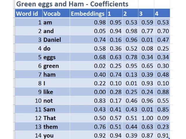
So you can see here that it's got the RMSE down to 0.4, so for example the first one predicted 3, it's actually 2, 4.5, 4.6, 5 and so forth, so you get the idea of how it works. Word embeddings work exactly the same way. So inspired by one of the students who talked about this during the week, I grabbed the text of Green Eggs and Ham.

And so here is the text of Green Eggs and Ham. I am Daniel, I am Sam, Sam I am, that's Sam I am, etc. And I've turned this poem into a matrix. And the way I did that was to take every unique word in that poem. Here is the ID of each of those words, just index from 1.

And so then I just randomly generated an embedding matrix, I equally well could have used the downloaded glove embeddings instead. And so then just for each word, I just look up in the list to find that word and find out what number it is, so I is number 8, and so here is the 8th row of the embedding matrix.

So you can see here that we've started with a poem and we've turned it into a matrix of floats. And so the reason we do this is because our machine learning tools want a matrix of floats, not a poem. So all of the questions about does it matter what the word IDs are, you can see it doesn't matter at all.

All we're doing is we're looking them up in this matrix and returning the floats. And once we've done that, we never use them again, we just use this matrix of floats. So that's what embeddings are. So I hope that's helpful. Feel free to ask if you have any questions either now or at any other time because we're going to be using embeddings throughout this class.

So hopefully that helped a few people clarify what's going on. So let's get back to recurrent neural networks. So to remind you, we talked about the purpose of recurrent neural networks as being really all about memory. So it's really all about this idea of memory. If we're going to handle something like recognizing a comment start and a comment end, and being able to keep track of the fact that we're in a comment for all of this time so that we can do modeling on this kind of structured language data, we're really going to need memory.

That allows us to handle long-term dependencies and it provides this stateful representation. So in general, the stuff we're talking about, we're going to be looking at things that kind of particularly need these three things. And it's also somewhat helpful just for when you have a variable length sequence. Questions about embeddings?

One is how does the size of my embedding depend on the number of unique words? So mapping green eggs and ham to five real numbers seems sufficient but wouldn't be for all of JRR Tolkien. So your choice of how big to make your embedding matrix, as in how many latent factors to create, is one of these architectural decisions which we don't really have an answer to.

My best suggestion is to read the Word2Vec paper which introduced a lot of this and look at the difference between a 50 dimensional, 100 dimensional, 200, 300, 600 dimensional and see what are the different levels of accuracy that those different size embedding matrices created when the authors of that paper provided this information.

So that's a quick shortcut because other people have already experimented and provided those results for you. The other is to do your own experiments, try a few different sizes. It's not really about the length of the word list, it's really about the complexity of the language or other problem that you're trying to solve.

That's really problem dependent and will require both your intuition developed from reading and experimenting and also your own experiments. And what would be the range of root mean squared error value to say that a model is good? To say that a model is good is another model specific issue.

So a root mean squared error is very interpretable, it's basically how far out is it on average. So we were finding that we were getting ratings within about 0.4, this mini Excel dataset is too small to really make intelligent comments, but let's say it was bigger. If we're getting within 0.4 on average, that sounds like it's probably good enough to be useful for helping people find movies that they might like.

But there's really no one solution, I actually wrote a whole paper about this. If you look up "Designing Great Data Products" and look at my name, this is based on really mainly 10 years of work I did at a company I created called Optimal Decision Group. And Optimal Decision Group was all about how to use predictive modeling not just to make predictions but to optimize actions, and this whole paper is about that.

In the end, it's really about coming up with a way to measure the benefit to your organization or to your project of getting that extra 0.1% accuracy, and there are some suggestions on how to do that in this paper. So we looked at a kind of a visual vocabulary that we developed for writing down neural nets where any colored box represents a matrix of activations, that's a really important point to remember.

A colored box represents a matrix of activations, so it could either be the input matrix, it could be the output matrix, or it could be the matrix that comes from taking an input and putting it through like a matrix product. The rectangle boxes represent inputs, the circular ones represent hidden, so intermediate activations, and the triangles represent outputs.

Arrows, very importantly, represent what we'll call layer operations. And a layer operation is anything that you do to one colored box to create another colored box. In general, it's almost always going to involve some kind of linear function like a matrix product or convolution, and it will probably also include some kind of activation function like ReLU or softmax.

Because the activation functions are pretty unimportant in terms of detail, I started removing those from the pictures as we started to look at more complex models. And then in fact, because the layer operations actually are pretty consistent, we probably know what they are, I started removing those as well, just to keep these simple.

And so we're simplifying these diagrams to try and just keep the main pieces. And as we did so, we could start to create more complex diagrams. And so we talked about a kind of language model where we would take inputs of a character, character number 1 and character number 2, and we would try and predict character number 3.

And so we thought one way to do that would be to create a deep neural network with two layers. The character 1 input would go through a layer operation to create our first fully connected layer. That would go through another layer operation to create a second fully connected layer.

And we would also add our second character input going through its own fully connected layer at this point. And to recall, the last important thing we have to learn is that two arrows going into a single shape means that we are adding the results of those two layer operations together.

So two arrows going into a shape represents summing up, element-wise, the results of these two layer operations. So this was the kind of little visual vocabulary that we set up last week. And I've kept track of it down here as to what the things are in case you forget.

So now I wanted to point out something really interesting, which is that there's three kinds of layer operations going on. Here I'm expanding this now. We've got predicting a fourth character of a sequence using characters 1, 2 and 3. It's exactly the same method as on the previous slide.

There are layer operations that turn a character input into a hidden activation matrix. There's one here, here's one here. There are layer operations that turn one hidden layer activation into a new hidden layer activation. And then there's an operation that takes hidden activations and turns it into output activations.

And so you can see here, I've colored them in. And here I've got a little legend of these different colors. Green are the input to hidden, blue is the output, and orange is the hidden to hidden. So my claim is that the dimensions of the weight matrices for each of these different colored arrows, all of the green ones have the same dimensions because they're taking an input of vocab size and turning it into an output hidden activation of size number of activations.

So all of these arrows represent weight matrices which are of the same dimensionality. Ditto, the orange arrows represent weight matrices with the same dimensionality. I would go further than that though and say the green arrows represent semantically the same thing. They're all saying how do you take a character and convert it into a hidden state.

And the orange arrows are all saying how do you take a hidden state from a previous character and turn it into a hidden state for a new character. And then the blue one is saying how do you take a hidden state and turn it into an output. When you look at it that way, all of these circles are basically the same thing, they're just representing this hidden state at a different point in time.

And I'm going to use this word 'time' in a fairly general way, I'm not really talking about time, I'm just talking about the sequence in which we're presenting additional pieces of information to this model. We first of all present the first character, the second character and the third character.

So we could redraw this whole thing in a simpler way and a more general way. Before we do, I'm actually going to show you in Keras how to build this model. And in doing so, we're going to learn a bit more about the functional API which hopefully you'll find pretty interesting and useful.

To do that, we are going to use this corpus of all of the collected works of niche shape. So we load in those works, we find all of the unique characters of which there are 86. Here they are, joined up together, and then we create a mapping from the character to the index at which it appears in this list and a mapping from the index to the character.

So this is basically creating the equivalent of these tables, or more specifically I guess this table. But rather than using words, we're looking at characters. So that allows us to take the text of Nietzsche and convert it into a list of numbers where the numbers represent the number at which the character appears in this list.

So here are the first 10. So at any point we can turn this, that's called IDX, so we've converted our whole text into the equivalent indices. At any point we can turn it back into text by simply taking those indexes and looking them up in our index to character mapping.

So here you can see we turn it back into the start of the text again. So that's the data we're working with. The data we're working with is a list of character IDs at this point where those character IDs represent the collected works of Nietzsche. So we're going to build a model which attempts to predict the fourth character from the previous three.

So to do that, we're going to go through our whole list of indexes from 0 up to the end minus 3. And we're going to create a whole list of the 0th, 4th, 8th, 12th etc characters and a list of the 1st, 5th, 9th etc and the 2nd, 6th, 10th and so forth.

So this is going to represent the first character of each sequence, the second character of each sequence, the third character of each sequence and this is the one we want to predict, the fourth character of each sequence. So we can now turn these into NumPy arrays just by stacking them up together.

And so now we've got our input for our first characters, second characters and third characters of every four character piece of this collected works. And then our y's, our labels, will simply be the fourth characters of each sequence. So here you can see them. So for example, if we took x1, x2 and x3 and took the first element of each, this is the first character of the text, the second character of the text, the third character of the text and the fourth character of the text.

So we'll be trying to predict this based on these three. And then we'll try to predict this based on these three. So that's our data format. So you can see we've got about 200,000 of these inputs for each of x1 through x3 and for y. And so as per usual, we're going to first of all turn them into embeddings by creating an embedding matrix.

I will mention this is not normal. I haven't actually seen anybody else do this. Most people just treat them as one-hot encodings. So for example, the most widely used blog post about car RNNs, which really made them popular, was Andre Kepathys, and it's quite fantastic. And you can see that in his version, he shows them as being one-hot encoder.

We're not going to do that, we're going to turn them into embeddings. I think it makes a lot of sense. Capital A and lowercase a have some similarities that an embedding can understand. Different types of things that have to be opened and closed, like different types of parentheses and quotes, have certain characteristics that can be constructed in embedding.

There's all kinds of things that we would expect an embedding to capture. So my hypothesis was that an embedding is going to do a better job than just a one-hot encoding. In my experiments over the last couple of weeks, that generally seems to be true. So we're going to take each character, 1-3, and turn them into embeddings by first creating an input layer for them and then creating an embedding layer for that input.

And then we can return the input layer and the flattened version of the embedding layer. So this is the input to an output of each of our three embedding layers for our three input characters. So that's basically our inputs. So we now have to decide how many activations do we want.

And so that's something we can just pick. So I've decided to go with 256. That's something that seems reasonable, seems to have worked okay. So we now have to somehow construct something where each of our green arrows ends up with the same weight matrix. And it turns out Keras makes this really easy with the Keras Functional API.

When you call dense like this, what it's actually doing is it's creating a layer with a specific weight matrix. Notice that I haven't passed in anything here to say what it's connected to, so it's not part of a model yet. This is just saying, I'm going to have something which is a dense layer which creates 256 activations and I'm going to call it dense_in.

So it doesn't actually do anything until I then do this, so I connect it to something. So here I'm going to say character1's hidden state comes from taking character1, which was the output of our first embedding, and putting it through this dense_in layer. So this is the thing which creates our first circle.

So the embedding is the thing that creates the output of our first rectangle, this creates our first circle. And so dense_in is the green arrow. So what that means is that in order to create the next set of activations, we need to create the orange arrow. So since the orange arrow is different weight matrix to the green arrow, we have to create a new dense layer.

So here it is. I've got a new dense layer, and again, with n hidden outputs. So by creating a new dense layer, this is a whole separate weight matrix, this is going to keep track of. So now that I've done that, I can create my character2 hidden state, which is here, and I'm going to have to sum up two separate things.

I'm going to take my character2 embedding, put it through my green arrow, dense_in, that's going to be there. I'm going to take the output of my character1's hidden state and run it through my orange arrow, which we call dense_hidden, and then we're going to merge the two together. And merge by default does a sum.

So this is adding together these two outputs. In other words, it's adding together these two layer operation outputs. And that gives us this circle. So the third character output is done in exactly the same way. We take the third character's embedding, run it through our green arrow, take the result of our previous hidden activations and run it through our orange arrow, and then merge the two together.

Question- Is the first output the size of the latent fields in the embedding? Answer- The size of the latent embeddings we defined when we created the embeddings up here, and we defined them as having nFAT size, and nFAT we defined as 42. So C1, C2 and C3 represent the result of putting each character through this embedding and getting out 42 latent factors.

Those are then the things that we put into our green arrow. So after doing this three times, we now have C3 hidden, which is 1, 2, 3 here. So we now need a new set of weights, we need another dense layer, the blue arrow. So we'll call that "dense out".

And this needs to create an output of size 86, vocab size, we need to create something which can match to the one-hot encoded list of possible characters, which is 86 long. So now that we've got this orange arrow, we can apply that to our final hidden state to get our output.

So in Keras, all we need to do now is call model "passing in" the three inputs, and so the three inputs were returned to us way back here. Each time we created an embedding, we returned the input layer, so C1 in C2 in C3 input. So passing in the three inputs, and passing in our output.

So that's our model. And so we can now compile it, set a learning rate, fit it, and as you can see, its loss is gradually decreasing. And we can then test that out very easily by creating a little function that we're going to pass three letters. We're going to take those three letters and turn them into character indices, just look them up to find the indexes, turn each of those into a numpy array, call model.predict on those three arrays.

That gives us 86 outputs, which we then do argmax to find which index into those 86 is the highest, and that's the character number that we want to return. So if we pass in PHI, it thinks that L is most likely next, space th is most likely next, space an, it thinks that d is most likely next.

So you can see that it seems to be doing a pretty reasonable job of taking three characters and returning a fourth character that seems pretty sensible, not the world's most powerful model, but a good example of how we can construct pretty arbitrary architectures using Keras and then letting SGD do the work.

This model, how would it consider the context in which we are trying to predict the next context, it knows nothing about the context, all it has at any point in time is the previous three characters. So it's not a great model. We're going to improve it though, we've got to start somewhere.

In order to answer your question, let's build this up a little further, and rather than trying to predict character 4 from the previous three characters, let's try and predict character n from the previous n-1 characters. And since all of these circles basically mean the same thing, which is the hidden state at this point, and since all of these orange arrows are literally the same thing, it's a dense layer with exactly the same weight matrix, let's take all of the circles on top of each other, which means that these orange arrows then can just become one arrow pointing into itself.

And this is the definition of a recurrent neural network. When we see it in this form, we say that we're looking at it in its recurrent form. When we see it in this form, we can say that we're looking at it in its unrolled form, or unfolded form. They're both very common.

This is obviously neater. And so for quickly sketching out an RNN architecture, this is much more convenient. But actually, this unrolled form is really important. For example, when Keras uses TensorFlow as a backend, it actually always unrolls it in this way in order to compute it. That obviously takes up a lot more memory.

And so it's quite nice being able to use the Theano backend with Keras which can actually directly implement it as this kind of loop, and that's what we'll be doing today shortly. But in general, we've got the same idea. We're going to have character 1 input come in, go through the first green arrow, go through the first orange arrow, and from then on, we can just say take the second character, repeat the third character, repeat, and at each time period, we're getting a new character going through a layer operation, as well as taking the previous hidden state and putting it through its layer operation.

And then at the very end, we will put it through a different layer operation, the blue arrow, to get our output. So I'm going to show you this in Keras now. Does every fully connected layer have to have the same activation function? In general, no, in all of the models we've seen so far, we have constructed them in a way where you can write anything you like as the activation function.

In general though, I haven't seen any examples of successful architectures which mix activation functions other than at the output layer would pretty much always be a softmax for classification. I'm not sure it's not something that might become a good idea, it's just not something that anybody has done very successfully with so far.

I will mention something important about activation functions though, which is that you can use pretty much almost any nonlinear function as an activation function and get pretty reasonable results. There are actually some pretty cool papers that people have written where they've tried all kinds of weird activation functions and they pretty much all work.

So it's not something to get hung up about. It's more just certain activation functions will train more quickly and more resiliently. In particular, ReLU and ReLU variations tend to work particularly well. So let's implement this. So we're going to use a very similar approach to what we used before.

And we're going to create our first RNN and we're going to create it from scratch using nothing but standard Keras dense layers. In this case, we can't create C1, C2 and C3, we're going to have to create an array of our inputs. We're going to have to decide what N we're going to use, and so for this one I've decided to use 8, so CS is characters, so I'm going to use 8 characters to predict the 9th character.

So I'm going to create an array with 8 elements in it, and each element will contain a list of the 0, 8, 16, 24th character, the 1, 9, 17, etc. character, the 2, 10, 18, etc. character, just like before. So we're going to have a sequence of inputs where each one is offset by 1 from the previous one, and then our output will be exactly the same thing, except we're going to look at the index to cross by CS, so 8.

So this will be the 8th thing in each sequence and we're going to predict it with the previous ones. So now we can go through every one of those input data items, lists, and turn them into a NumPy array, and so here you can see that we have 8 inputs, and each one is at length 75,000 or so.

Do the same thing for our y, get a NumPy array out of it, and here we can visualize it. So here are the first 8 elements of x, so in looking at the first 8 elements of x, let's look at the very first element of each one, 40, 42, 29.

So this column is the first 8 characters of our text, and here is the 9th character. So the first thing that the model will try to do is to look at these 8 to predict this, and then look at these 8 to predict this, and look at these 8 and predict this and so forth.

And indeed you can see that this list here is exactly the same as this list here. The final character of each sequence is the same as the first character of the next sequence. So it's almost exactly the same as our previous data, we've just done it in a more flexible way.

We'll create 43 latent factors as before, where we use exactly the same embedding input function as before. And again, we're just going to have to use lists to store everything. So in this case, all of our embeddings are going to be in a list, so we'll go through each of our characters and create an embedding input and output for each one, store it here.

And here we're going to define them all at once, our green arrow, orange arrow, and blue arrow. So here we're basically saying we've got 3 different weight matrices that we want Keras to keep track of for us. So the very first hidden state here is going to take the list of all of our inputs, the first one of those, and then that's a tuple of two things.

The first is the input to it, and the second is the output of the embedding. So we're going to take the output of the embedding for the very first character, pass that into our green arrow, and that's going to give us our initial hidden state. And then this looks exactly the same as we saw before, but rather than doing it listing separately, we're just going to loop through all of our remaining 1 through 8 characters and go ahead and create the green arrow, orange arrow, and add the two together.

So finally we can take that final hidden state, put it through our blue arrow to create our final output. So we can then tell Keras that our model is all of the embedding inputs for that list we created together, that's our inputs, and then our output that we just created is the output.

And we can go ahead and fit that model. So we would expect this to be more accurate because it's now got 8 pieces of context in order to predict. So previously we were getting this time we get down to 1.8. So it's still not great, but it's an improvement and we can create exactly the same kind of tests as before, so now we can pass in 8 characters and get a prediction of the ninth.

And these all look pretty reasonable. So that is our first RNN that we've now built from scratch. This kind of RNN where we're taking a list and predicting a single thing is most likely to be useful for things like sentiment analysis. Remember our sentiment analysis example using IMDB? So in this case we were taking a sequence, being a list of words in a sentence, and predicting whether or not something is positive sentiment or negative sentiment.

So that would seem like an appropriate kind of use case for this style of RNN. So at that moment my computer crashed and we lost a little bit of the class's video. So I'm just going to fill in the bit that we missed here. So I wanted to show you something kind of interesting, which you may have noticed, which is when we created our hidden dense layer, that is our orange arrow, I did not initialize it in the default way which is the GLORO initialization, but instead I said "init = identity".

You may also have noticed that the equivalent thing was shown in our Keras RNN. This here where it says "inner init = identity" was referring to the same thing. It's referring to what is the initialization that is used for this orange arrow, how are those weights originally initialized. So rather than initializing them randomly, we're going to initialize them with an identity matrix.

An identity matrix, you may recall from your linear algebra at school, is a matrix which is all zeros, except it is just ones down the diagonal. So if you multiply any matrix by the identity matrix, it doesn't change the original matrix at all. You can write back exactly what you started with.

So in other words, we're going to start off by initializing our orange arrow, not with a random matrix, but with a matrix that causes the hidden state to not change at all. That makes some intuitive sense. It seems reasonable to say "well in the absence of other knowledge to the country, why don't we start off by having the hidden state stay the same until the SGD has a chance to update that." But it actually turns out that it also makes sense based on an empirical analysis.

So since we always only do things that Jeffrey Hinton tells us to do, that's good news because this is a paper by Jeff Hinton in which he points out this rather neat trick which is if you initialize an RNN with the hidden weight matrix initialized to an identity matrix and use rectified linear units as we are here, you actually get an architecture which can get fantastic results on some reasonably significant problems including speech recognition and language modeling.

I don't see this paper referred to or discussed very often, even though it is well over a year old now. So I'm not sure if people forgot about it or haven't noticed it or what, but this is actually a good trick to remember is that you can often get quite a long way doing nothing but an identity matrix initialization and rectified linear units in just as we have done here to set up our architecture.

Okay, so that's a nice little trick to remember. And so the next thing we're going to do is to make a couple of minor changes to this diagram. So the first change we're going to make is we're going to take this rectangle here, so this rectangle is referring to what is it that we repeat and so since in this case we're predicting character n from characters 1 through n minus 1, then this whole area here we're looping from 2 to n minus 1 before we generate our output once again.

So what we're going to do is we're going to take this triangle and we're going to put it inside the loop, put it inside the rectangle. And so what that means is that every time we loop through this, we're going to generate another output. So rather than generating one output at the end, this is going to predict characters 2 through n using characters n1 through n minus 1.

So it's going to predict character 2 using character 1 and character 3 using characters 1 and 2 and character 4 using characters 1, 2 and 3 and so forth. And so that's what this model would do. It's nearly exactly the same as the previous model, except after every single step after creating the hidden state on every step, we're going to create an output every time.

So this is not going to create a single output like this does, which predicted a single character, the last character, in fact, the next after the last character of the sequence, character n using characters 1 through n minus 1. This is going to predict a whole sequence of characters 2 through n using characters 1 through n minus 1.

OK, so that was all the stuff that we'd lost when we had our computer crash. So let's now go back to the lesson. Let's now talk about how we would implement this sequence, where we're going to predict characters 2 through n using characters 1 through n minus 1. Now why would this be a good idea?

There's a few reasons, but one obvious reason why this would be a good idea is that if we're only predicting one output for every n inputs, then the number of times that our model has the opportunity to back-propagate those in gradients and improve those weights is just once for each sequence of characters.

Whereas if we predict characters 2 through n using characters 1 through n minus 1, we're actually getting a whole lot of feedback about how our model is going. So we can back-propagate n times, or actually n minus 1 times every time we do another sequence. So there's a lot more learning going on for nearly the same amount of computation.

The other reason this is handy is that as you'll see in a moment, it's very helpful for creating RNNs which can do truly long-term dependencies or context, as one of the people asking a question earlier described it. So we're going to start here before we look at how to do context.

And so really anytime you're doing a kind of sequence-to-sequence exercise, you probably want to construct something of this format where your triangle is inside the square rather than outside the square. It's going to look very similar, and so I'm calling this returning sequences, rather than returning a single character, we're going to return a sequence.

And really, most things are the same. Our character_in data is identical to before, so I've just commented it out. And now our character_out output isn't just a single character, but it's actually a list of 8 sequences again. In fact, it's exactly the same as the input, except that I have removed the -1, so it's just shifted over by 1.

In each sequence, the first character will be used to predict the second, the first and second will predict the third, the first, second and third will predict the fourth and so forth. So we've got a lot more predictions going on, and therefore a lot more opportunity for the model to learn.

So then we will create our y's just as before with our x's. And so now our y dataset looks exactly like our x dataset did, but everything's just shifted across by one character. And the model's going to look almost identical as well. We've got our three dense layers as before, but we're going to do one other thing different to before.

Rather than treating the first character as special, I won't treat it as special. I'm going to move the character into here, so rather than repeating from 2 to n-1, I'm going to repeat from 1 to n-1. So I've moved my first character into here. So the only thing I have to be careful of is that we have to somehow initialize our hidden state to something.

So we're going to initialize our hidden state to a vector of zeros. So here we do that, we say we're going to have something to initialize our hidden state, which we're going to feed it with a vector of zeros shortly. So our initial hidden state is just going to be the result of that.

And then our loop is identical to before, but at the end of every loop, we're going to append this output. So we're now going to have 8 outputs for every sequence rather than 1. And so now our model has two changes. The first is it's got an array of outputs, and the second is that we have to add the thing that we're going to use to store our vector of zeros somewhere, so we're going to put this into our input as well.

The box refers to the area that we're looping. So initially we repeated the character n input coming into here, and then the hidden state coming into itself from 2 to n-1. So the box is the thing which I'm looping through all those times. This time I'm looping through this whole thing.

So a character input coming in, generating the hidden state, and creating an output, repeating that whole thing every time. And so now you can see creating the output is inside the loop rather than outside the loop. So therefore we end up with an array of outputs. So our model's nearly exactly the same as before, it's just got these two changes.

So now when we fit our model, we're going to add an array of zeros to the start of our inputs. Our outputs are going to be those lists of 8 that have been offset by 1, and we can go ahead and train this. And you can see that as we train it, now we don't just have one loss, we have 8 losses.

And that's because every one of those 8 outputs has its own loss. How are we going at predicting character 1 in each sequence? 2, 3, 4. And as you would expect, our ability to predict the first character using nothing but a vector of zeros is pretty limited. So that very quickly flattens out.

Whereas our ability to predict the 8th character, it has a lot more context. It has 7 characters of context. And so you can see that the 8th character's loss keeps on improving. And indeed, by a few epochs, we have a significantly better loss than we did before. So this is what a sequence model looks like.

And so you can see a sequence model when we test it. We pass in a sequence like this, space this is, and after every character, it returns its guess. So after seeing a space, it guesses the next will be a t. After seeing a space t, it guesses the next will be an h.

After seeing a space th, it guesses the next will be an e and so forth. And so you can see that it's predicting some pretty reasonable things here, and indeed quite often there, what actually happened. So after seeing space par t, it expects that will be the end of the word, and indeed it was.

So after seeing par t, it's guessing that the next word is going to be of, and indeed it was. So it's able to use sequences of 8 to create a context, which isn't brilliant, but it's an improvement. So how do we do that same thing with Keras? With Keras, it's identical to our previous model, except that we have to use the different input and output arrays, just like I just showed you, so the whole sequence of labels and the whole sequence of inputs.

And then the second thing we have to do is add one parameter, which is return_sequences_equals_true. return_sequences_equals_true simply says rather than putting the triangle outside the loop, put the triangle inside the loop. And so return an output from every time you go to another time step rather than just returning a single output at the end.

So it's that easy in Keras. I add this return_sequences_equals_true, I don't have to change my data at all other than some very minor dimensionality changes, and then I can just go ahead and fit it. As you can see, I get a pretty similar loss function to what I did before, and I can build something that looks very much like we had before and generate some pretty similar results.

So that's how we create a sequence model with Keras. So then the question of how do you create more state, how do you generate a model which is able to handle long-term dependencies. To generate a model that understands long-term dependencies, we can't anymore present our pieces of data at random.

So so far, we've always been using the default model, which is shuffle=true. So it's passing across these sequences of 8 in a random order. If we're going to do something which understands long-term dependencies, the first thing we are going to have to do is we're going to have to use shuffle=false.

The second thing we're going to have to do is we're going to have to stop passing in an array of zeros as my starting point every time around. So effectively what I want to do is I want to pass in my array of zeros right at the very start when I first start training, but then at the end of my sequence of 8, rather than going back to initialize to zeros, I actually want to keep this hidden state.

So then I'd start my next sequence of 8 with this hidden state exactly where it was before, and that's going to allow it to basically build up arbitrarily long dependencies. So in Keras, that's actually as simple as adding one additional parameter, and the additional parameter is called stateful. And so when you say stateful=true, what that tells Keras is at the end of each sequence, don't reset the hidden activations to zero, but leave them as they are.

And that means that we have to make sure we pass shuffle=false when we train it, so it's now going to pass the first 8 characters of the book and then the second 8 characters of the book and then the third 8 characters of the book, leaving the hidden state untouched between each one, and therefore it's allowing it to continue to build up as much state as it wants to.

Training these stateful models is a lot harder than training the models we've seen so far. And the reason is this. In these stateful models, this orange arrow, this single weight matrix, it's being applied to this hidden matrix not 8 times, but 100,000 times or more, depending on how big your text is.

And just imagine if this weight matrix was even slightly poorly scaled, so if there was like one number in it which was just a bit too high, then effectively that number is going to be to the power of 100,000, it's being multiplied again and again and again. So what can happen is you get this problem they call exploding gradients, or really in some ways it's better described as exploding activations.

Because we're multiplying this by this almost the same weight matrix each time, if that weight matrix is anything less than perfectly scaled, then it's going to make our hidden matrix disappear off into infinity. And so we have to be very careful of how to train these, and indeed these kinds of long-term dependency models were thought of as impossible to train for a while, until some folks in the mid-90s came up with a model called the LSTM, or Long Short-Term Memory.

And in the Long Short-Term Memory, and we'll learn more about it next week, and we're actually going to implement it ourselves from scratch, we replace this loop here with a loop where there is actually a neural network inside the loop that decides how much of this state matrix to keep and how much to use at each activation.

And so by having a neural network which actually controls how much state is kept and how much is used, it can actually learn how to avoid those gradient explosions, it can actually learn how to create an effective sequence. So we're going to look at that a lot more next week, but for now I will tell you that when I tried to run this using a simple RNN, even with an identity matrix, initialization and reuse, I had no luck at all.

So I had to replace it with an LSTM. Even that wasn't enough, I had to have well-scaled inputs, so I added a batch normalization layer after my embeddings. And after I did those things, then I could fit it. It still ran pretty slowly, so before I was getting 4 seconds per epoch, now it's 13 seconds per epoch, and the reason here is it's much harder to parallelize this.

It has to do each sequence in order, so it's going to be slower. But over time, it does eventually get substantially better loss than I had before, and that's because it's able to keep track of and use this state. That's a good question. Definitely maybe. There's been a lot of discussion and papers about this recently.

There's something called layer normalization, which is a method which is explicitly designed to work well with RNNs. Standard batch norm doesn't. It turns out it's actually very easy to do layer normalization with Keras using a couple of simple parameters you can provide for the normal batch norm constructor. In my experiments, that hasn't worked so well, and I will show you a lot more about that in just a few minutes.

Stateful models are great. We're going to look at some very successful stateful models in just a moment, but just be aware that they are more challenging to train. You'll see another thing I had to do here is I had to reduce the learning rate in the middle, again because you just have to be so careful of these exploding gradient problems.

Let me show you what I did with this, which is I tried to create a stateful model which worked as well as I could. I took the same Nietzsche data as before, and I tried splitting it into chunks of 40 rather than 8, so each one could do more work.

Here are some examples of those chunks of 40. I built a model that was slightly more sophisticated than the previous one in two ways. The first is it has an RNN feeding into an RNN. That's kind of a crazy idea, so I've drawn a picture. An RNN feeding into an RNN means that the output is no longer going to an output, it's actually the output of the first RNN is becoming the input to the second RNN.

So the character input goes into our first RNN and has the state updates as per usual, and then each time we go through the sequence, it feeds the result to the state of the second RNN. Why is this useful? Well, because it means that this output is now coming from not just a single dense matrix and then a single dense matrix here, it's actually going through one, two, three dense matrices and activation functions.

So I now have a deep neural network, assuming that two layers get to count as deep, between my first character and my first output. And then indeed, between every hidden state and every output, I now have multiple hidden layers. So effectively, what this is allowing us to do is to create a little deep neural net for all of our activations.

That turns out to work really well because the structure of language is pretty complex and so it's nice to be able to give it a more flexible function that it can learn. That's the first thing I do. It's this easy to create that. You just copy and paste whatever your RNN line is twice.

You can see I've now added dropout inside my RNN. And as I talked about before, adding dropout inside your RNN turns out to be a really good idea. There's a really great paper about that quite recently showing that this is a great way to regularize an RNN. And then the second change I made is rather than going straight from the RNN to our output, I went through a dense layer.

Now there's something that you might have noticed here is that our dense layers have this extra word at the front. Why do they have this extra word at the front? Time distributed. It might be easier to understand why by looking at this earlier sequence model with Keras. And note that the output of our RNN is not just a vector of length 256, but 8 vectors of length 256 because it's actually predicting 8 outputs.

So we can't just have a normal dense layer because a normal dense layer needs a single dimension that it can squish down. So in this case, what we actually want to do is create 8 separate dense layers at the output, one for every one of the outputs. And so what time distributed does is it says whatever the layer is in the middle, I want you to create 8 copies of them, or however long this dimension is.

And every one of those copies is going to share the same weight matrix, which is exactly what we want. So the short version here is in Keras, anytime you say return_sequences=true, any dense layers you have after that will always have to have time distributed wrapped around them because we want to create not just one dense layer, but 8 dense layers.

So in this case, since we're saying return_sequences=true, we then have a time distributed dense layer, some dropout, and another time distributed dense layer. I have a few questions. Does the first RNN complete before it passes to the second or is it layer by layer? No, it's operating exactly like this.

So my initialization starts, my first character comes in, and at the output of that comes two things, the hidden state for my next hidden state and the output that goes into my second LSTM. The best way to think of this is to draw it in the unrolled form, and then you'll realize there's nothing magical about this at all.

In an unrolled form, it just looks like a pretty standard deep neural net. What's dropout_u and dropout_w? We'll talk about that more next week. In an LSTM, I mentioned that there's kind of like little neural nets that control how the state updates work, and so this is talking about how the dropout works inside these little neural nets.

And when stateful is false, can you explain again what is reset after each training example? The best way to describe that is to show us doing it. Remember that the RNNs that we built are identical to what Keras does, or close enough to identical. Let's go and have a look at our version of return sequences.

You can see that what we did was we created a matrix of zeros that we stuck onto the front of our inputs. Every set of 8 characters now starts with a vector of zeros. In other words, this initialize to zeros happens every time we finish a sequence. In other words, this hidden state gets initialized to 0 at the end of every sequence.

It's this hidden state which is where all of these dependencies and state is kept. So doing that is resetting the state every time we look at a new sequence. So when we say stateful = false, it only does this initialize to 0 once at the very start, or when we explicitly ask it to.

So when I actually run this model, the way I do it is I wrote a little thing called run epochs that goes model.resetStates and then does a fit on one epoch, which is what you really want at the end of your entire works of Nietzsche. You want to reset the state because you're about to go back to the very start and start again.

So with this multilayer LSTM going into a multilayer neural net, I then tried seeing how that goes. And remember that with our simpler versions, we were getting 1.6 loss was the best we could do. After one epoch, it's awful. And now rather than just printing out one letter, I'm starting with a whole sequence of letters, which is that, and asking it to generate a sequence.

You can see it starts out by generating a pretty rubbishy sequence. One more question. In the double LSTM layer model, what is the input to the second LSTM in addition to the output of the first LSTM? In addition to the output of the first LSTM is the previous output of its own hidden state.

Okay, so after a few more epochs, it's starting to create some actual proper English words, although the English words aren't necessarily making a lot of sense. So I keep running epochs. At this point, it's learned how to start chapters. This is actually how in this book the chapters always start with a number and then an equal sign.

It hasn't learned how to close quotes apparently, it's not really saying anything useful. So anyway, I kind of ran this overnight, and I then seeded it with a large amount of data, so I seeded it with all this data, and I started getting some pretty reasonable results. Shreds into one's own suffering sounds exactly like the kind of thing that you might see.

Religions have acts done by man. It's not all perfect, but it's not bad. Interestingly, this sequence here, when I looked it up, it actually appears in his book. This makes sense, right? It's kind of overfitting in a sense. He loves talking in all caps, but he only does it from time to time.

So once it so happened to start writing something in all caps that looked like this phrase that only appeared once and is very unique, there was kind of no other way that it could have finished it. So sometimes you get these little rare phrases that basically it's plagiarized directly from each of them.

Now I didn't stop there because I thought, how can we improve this? And it was at this point that I started thinking about batch normalization. And I started fiddling around with a lot of different types of batch normalization and layer normalization and discovered this interesting insight, which is that at least in this case, the very best approach was when I simply applied batch normalization to the embedding layer.

When I applied batch normalization to the embedding layer, this is the training curve that I got. So over epochs, this is my loss. With no batch normalization on the embedding layer, this was my loss. And so you can see this was actually starting to flatten out. This one really wasn't, and this one was training a lot quicker.

So then I tried training it with batch norm on the embedding layer overnight, and I was pretty stunned by the results. This was my seeding text, and after 1000 epochs, this is what it came up with. And it's got all kinds of pretty interesting little things. Perhaps some morality equals self-glorification.

This is really cool. For there are holy eyes to Schopenhauer's blind. This is interesting. In reality, we must step above it. You can see that it's learnt to close quotes even when those quotes were opened a long time ago. So if we weren't using stateful, it would never have learnt how to do this.

I've looked up these words in the original text and pretty much none of these phrases appear. This is actually a genuinely, novelly produced piece of text. It's not perfect by any means, but considering that this is only doing it character by character, using nothing but a 42 long embedding matrix for each character and nothing but there's no pre-trained vectors, there's just a pretty short 600,000 character epoch, I think it's done a pretty amazing job of creating a pretty good model.

And so there's all kinds of things you could do with a model like this. The most obvious one would be if you were producing a software keyboard for a mobile phone, for example. You could use this to have a pretty accurate guess as to what they were going to type next and correct it for them.

You could do something similar on a word basis. But more generally, you could do something like anomaly detection with this. You could generate a sequence that is predicting what the rest of the sequence is going to look like for the next hour and then recognize if something falls outside of what your prediction was and you know there's been some kind of anomaly.

There's all kinds of things you can do with these kinds of models. I think that's pretty fun, but I want to show you something else which is pretty fun, which is to build an RNN from scratch in Theano. And what we're going to do is we're going to try and work up to next week where we're going to build an RNN from scratch in NumPy.

And we're also going to build an LSTM from scratch in Theano. And the reason we're doing this is because next week's our last class in this part of the course, I want us to leave with kind of feeling like we really understand the details of what's going on behind the scenes.

The main thing I wanted to teach in this class is the applied stuff, these kind of practical tips about how you build a sequence model. Use return equals true, put batch null in the embedding layer, add time distributed to the dense layer. But I also know that to really debug your models and to build your architectures and stuff, it really helps to understand what's going on.

Particularly in the current situation where the tools and libraries available are not that mature, they still require a whole lot of manual stuff. So I do want to try and explain a bit more about what's going on behind the scenes. In order to build an RNN in Theano, first of all make a small change to our Keras model, which is that I'm going to use One Hot encoding.

I don't know if you noticed this, but we did something pretty cool in all of our models so far, which is that we never actually One Hot encoded our output. Question 3. Will time distributed dense take longer to train than dense? And is it really that important to use time distributed dense?

So if you don't add time distributed dense to a model where return sequence equals true, it literally won't work. It won't compile. Because you're trying to predict eight things and the dense layer is going to stick that all into one thing. So it's going to say there's a mismatch in your dimensions.

But no, it doesn't really add much time because that's something that can be very easily paralyzed. And since a lot of things in RNNs can't be easily paralyzed, there generally is plenty of room in your GPU to do more work. So that should be fun. The short answer is you have to use it, otherwise it won't work.

I wanted to point out something which is that in all of our models so far, we did not One Hot encode our outputs. So our outputs, remember, looked like this. They were sequences of numbers. And so always before, we've had to One Hot encode our outputs to use them.

It turns out that Keras has a very cool loss function called sparse-categorical-cross-entropy. This is identical to categorical-cross-entropy, but rather than taking a One Hot encoded target, it takes an integer target, and basically it acts as if you had One Hot encoded it. So it basically does the indexing into it directly.

So this is a really helpful thing to know about because when you have a lot of output categories like, for example, if you're doing a word model, you could have 100,000 output categories. There's no way you want to create a matrix that is 100,000 long, nearly all zeros for every single word in your output.

So by using sparse-categorical-cross-entropy, you can just forget the whole One Hot encode. You don't have to do it. Keras implicitly does it for you, but without ever actually explicitly doing it, it just does a direct look up into the matrix. However, because I want to make things simpler for us to understand, I'm going to go ahead and recreate our Keras model using One Hot encoding.

So I'm going to take exactly the same model that we had before with return_sequences=true, but this time I'm going to use normal-categorical-cross-entropy, which means that -- and the other thing I'm doing is I don't have an embedding layer. So since I don't have an embedding layer, I also have to One Hot encode my inputs.

So you can see I'm calling 2-categorical on all my inputs and 2-categorical on all my outputs. So now the shape is 75,000 x 8, as before, by 86. So this is the One Hot encoding dimension with which there are 85 zeros and 1 1. So we fit this in exactly the same way, we get exactly the same answer.

So the only reason I was doing that was because I want to use One Hot encoding for the version that we're going to create ourselves from scratch. So we haven't really looked at Theano before, but particularly if you come back next year, as we start to try to add more and more stuff on top of Keras or into Keras, increasingly you'll find yourself wanting to use Theano, because Theano is the language, if you like, that Keras is using behind the scenes, and therefore it's the language which you can use to extend it.

Of course you can use TensorFlow as well, but we're using Theano in this course because I think it's much easier for this kind of application. So let's learn to use Theano. In the process of doing it in Theano, we're going to have to force ourselves to think through a lot more of the details than we have before, because Theano doesn't have any of the conveniences that Keras has.

There's no such thing as a variable. We have to think about all of the weight matrices and activation functions and everything else. So let me show you how it works. In Theano, there's this concept of a variable, and a variable is something which we basically define like so. We can say there is a variable which is a matrix which I will call T_input, and there is a variable which is a matrix that we'll call T_output, and there is a variable that is a vector that we will call H0.

What these are all saying is that these are things that we will give values to later. Programming in Theano is very different to programming in normal Python, and the reason for this is Theano's job in life is to provide a way for you to describe a computation that you want to do, and then it's going to compile it for the GPU, and then it's going to run it on the GPU.

So it's going to be a little more complex to work in Theano, because Theano isn't going to be something where we immediately say do this, and then do this, and then do this. Instead we're going to build up what's called a computation graph. It's going to be a series of steps.

We're going to say in the future, I'm going to give you some data, and when I do, I want you to do these steps. So rather than actually starting off by giving it data, we start off by just describing the types of data that when we do give it data, we're going to give it.

So eventually we're going to give it some input data, we're going to give it some output data, and we're going to give it some way of initializing the first hidden state. And also we'll give it a learning rate, because we might want to change it later. So that's all these things do.

They create Theano variables. So then we can create a list of those, and so this is all of the arguments that we're going to have to provide to Theano later on. So there's no data here, nothing's being computed, we're just telling Theano that these things are going to be used in the future.

The next thing that we need to do, because we're going to try to build this, is we're going to have to build all of the pieces in all of these layer operations. So specifically we're going to have to create the weight vector and bias matrix for the orange arrow, the weight vector and the bias matrix for the green arrow, the weight matrix and the bias vector for the orange arrow, the weight matrix and the bias vector for the green arrow, and the weight matrix and the bias vector for the blue arrow, because that's what these layer operations are.

They're a matrix multiplier followed by a non-linear activation function. So I've created some functions to do that. WH is what I'm going to call the weights and bias to my hidden layer, Wx will be my weights and bias to my input, and Wy will be my weights and bias to my output.

So to create them, I've created this little function called weights and bias in which I tell it the size of the matrix that I want to create. So the matrix that goes from input to hidden therefore has n input rows and n hidden columns. So weights and bias is here, and it's going to return a tuple, it's going to return our weights, and it's going to return our bias.

So how do we create the weights? To create the weights, we first of all calculate the magic Glorow number, the square root of 2 over fan n, so that's the scale of the random numbers that we're going to use. We then create those random numbers using the numpy_normal_random_number function, and then we use a special Theano keyword called 'shared'.

What shared does is it says to Theano, this data is something that I'm going to want you to pass off to the GPU later and keep track of. So as soon as you wrap something in shared, it kind of belongs to Theano now. So here is a weight matrix that belongs to Theano, here is a vector of zeros that belongs to Theano and that's our initial bias.

So we've initialized our weights and our bias, so we can do that for our inputs and we can do that for our outputs. And then for our hidden, which is the orange error, we're going to do something slightly different which is we will initialize it using an identity matrix.

And rather amusingly in numpy, it is 'i' for identity. So this is an identity matrix, believe it or not, of size n by n. And so that's our initial weights and our initial bias is exactly as before. It's a vector of zeros. So you can see we've had to manually construct each of these 3 weight matrices and bias vectors.

It's nice to now stick them all into a single list. And Python has this thing called chain from iterable, which basically takes all of these tuples and dumps them all together into a single list. And so this now has all 6 weight matrices and bias vectors in a single list.

We have defined the initial contents of each of these arrows. And we've also defined kind of symbolically the concept that we're going to have something to initialize it with here, something to initialize it with here and some time to initialize it with here. So the next thing we have to do is to tell Theano what happens each time we take a single step of this RNN.

On the GPU, you can't use a for loop. The reason you can't use a for loop is because a GPU wants to be able to parallelize things and wants to do things at the same time. And a for loop by definition can't do the second part of the loop until it's done the first part of the loop.

I don't know if we'll get time to do it in this course or not, but there's a very neat result which shows that there's something very similar to a for loop that you can parallelize, and it's called a scan operation. A scan operation is something that's defined in a very particular way.

A scan operation is something where you call some function for every element of some sequence. And at every point, the function returns some output, and the next time through that function is called, it's going to get the output of the previous time you called it, along with the next element of the sequence.

So in fact, I've got an example of it. I actually wrote a very simple example of it in Python. Here is the definition of scan, and here is an example of scan. Let's start with the example. I want to do a scan, and the function I'm going to use is to add two things together.

And I'm going to start off with the number 0, and then I'm going to pass in a range of numbers from 0 to 4. So what scan does is it starts out by taking the first time through, it's going to call this function with that argument and the first element of this.

So it's going to be 0 plus 0 equals 0. The second time, it's going to call this function with the second element of this, along with the result of the previous call. So it will be 0 plus 1 equals 1. The next time through, it's going to call this function with the result of the previous call plus the next element of this range, so it will be 1 plus 2 equals 3.

So you can see here, this scan operation defines a cumulative sum. And so you can see the definition of scan here. We're going to be returning an array of results. Initially, we take our starting point, 0, and that's our initial value for the previous answer from scan. And then we're going to go through everything in the sequence, which is 0 through 4.

We're going to apply this function, which in this case was AddThingsUp, and we're going to apply it to the previous result along with the next element of the sequence. Stick the result at the end of our list, set the previous result to whatever we just got, and then go back to the next element of the sequence.

So it may be very surprising, I mean hopefully it is very surprising because it's an extraordinary result, but it is possible to write a parallel version of this. So if you can turn your algorithm into a scan, you can run it quickly on GPU. So what we're going to do is our job is to turn this RNN into something that we can put into this kind of format, into a scan.

So let's do that. So the function that we're going to call on each step through is the function called Step. And the function called Step is going to be something which hopefully will not be very surprising to you. It's going to be something which takes our input, x, it does a dot product by that weight matrix we created earlier, wx, and adds on that bias vector we created earlier.

And then we do the same thing, taking our previous hidden state, multiplying it by the weight matrix for the hidden state, and adding the biases for the hidden state, and then puts the whole thing through an activation function, relu. So in other words, let's go back to the unrolled version.

So we had one bit which was calculating our previous hidden state and putting it through the hidden state weight matrix. It was taking our next input and putting it through the input one and then adding the two together. So that's what we have here, the x by wx and the h by wh, and then adding the two together along with the biases, and then put that through an activation function.

So once we've done that, we now want to create an output every single time, and so our output is going to be exactly the same thing. It's going to take the result of that, which we called h, our hidden state, multiply it by the output's weight vector, adding on the bias, and this time we're going to use softmax.

So you can see that this sequence here is describing how to do one of these things. And so this therefore defines what we want to do each step through. And at the end of that, we're going to return the hidden state we have so far and our output. So that's what's going to happen each step.

So the sequence that we're going to pass into it is, well, we're not going to give it any data yet because remember, all we're doing is we're describing a computation. So for now, we're just telling it that it's going to be, it will be a matrix. So we're saying it will be a matrix, we're going to pass you a matrix.

It also needs a starting point, and so the starting point is, again, we are going to provide to you an initial value for our hidden state, but we haven't done it yet. And then finally in Theano, you have to tell it what are all of the other things that are passed to the function, and we're going to pass it that whole list of weights.

That's why we have here the x, the hidden, and then all of the weights and biases. So that's now described how to execute a whole sequence of steps for an RNN. So we've now described how to do this to Theano. We haven't given it any data to do it, we've just set up the computation.

And so when that computation is run, it's going to return two things because step returns two things. It's going to return the hidden state and it's going to return our output activations. So now we need to calculate our error. Our error will be the categorical cross-entropy, and so these things are all part of Theano.

You can see I'm using some Theano functions here. And so we're going to compare the output that came out of our scan, and we're going to compare it to what we don't know yet, but it will be a matrix. And then once you do that, add it all together.

Now here's the amazing thing. Every step we're going to want to apply SGD, which means every step we're going to want to take the derivative of this whole thing with respect to all of the weights and use that, along with the learning rate, to update all of the weights.

In Theano, that's how you do it. You just say, "Please tell me the gradient of this function with respect to these inputs." And Theano will symbolically, automatically calculate all of the derivatives for you. So that's very nearly magic, but we don't have to worry about derivatives because it's going to calculate them all for us.

So at this point, I now have a function that calculates our loss, and I have a function that calculates all of the gradients that we need with respect to all of the different weights and parameters that we have. So we're now ready to build our final function. Our final function, as input, takes all of our arguments, that is, these four things, which is the things we told it we're going to need later.

The thing that's going to create an output is the error, which was this output. And then at each step, it's going to do some updates. What are the updates going to do? The updates it's going to do is the result of this little function. And this little function is something that creates a dictionary that is going to map every one of our weights to that weight minus each one of our gradients times the learning rate.

So it's going to update every weight to itself minus its gradient times the learning rate. So basically what Theano does is it says, it's got this little thing called updates, it says every time you calculate the next step, I want you to change your shared variables as follows. So there's our list of changes to make.

And so that's it. So we use our one hot encoded x's and our one hot encoded y's, and we have to now manually create our own loop. Theano doesn't have any built-in stuff for us, so we're going to go through every element of our input and we're going to say let's call that function, so that function is the function that we just created, and now we have to pass in all of these inputs.

So we have to finally pass in a value for the initial hidden state, the input, the target, and the learning rate. So this is where we get to do it is when we finally call it here. So here's our initial hidden state, it's just a bunch of zeros, our input, our output, and our learning rate, which we set to 0.01.

And then I've just set it to something here that says every thousand times, print out the error. And so as you can see, over time, it learns. And so at the end of learning, I get a new theano function which takes some piece of input, along with some initial hidden state, and it produces not the loss, but the output.

Are we using gradient descent and not stochastic gradient descent here? We're using stochastic gradient descent with a mini-batch size of 1. So gradient descent without stochastic actually means you're using a mini-batch size of the whole data set. This is kind of the opposite of that. I think this is called online gradient descent.

So remember earlier on, we had this thing to calculate the vector of outputs. So now to do our testing, we're going to create a new function which goes from our input to our vector of outputs. And so our predictions will be to take that function, pass it in our initial hidden state, and some input, and that's going to give us some predictions.

So if we call it, we can now see, let's now grab some sequence of text, pass it to our function to get some predictions, and let's see what it does. So after t, it expected h, after th, it expected e, after th e, expected space, after th en, expected the space, after th en, question mark, it expected the space.

So you can see here that we have successfully built an RNN from scratch using Theano. That's been a very, very quick run-through. My goal really tonight is to kind of get to a point where you can start to look at this during the week and kind of see all the pieces.

Because next week, we're going to try and build an LSTM in Theano, which is going to mean that I want you by next week to start to feel like you've got a good understanding of what's going on. So please ask lots of questions on the forum, look at the documentation, and so forth.

And then the next thing we're going to do after that is we're going to build an RNN without using Theano. We're going to use pure NumPy. And that means that we're not going to be able to use t.grad, we're going to have to calculate the gradients by hand. So hopefully that will be a useful exercise in really understanding what's going on in that propagation.

So I kind of want to make sure you feel like you've got enough information to get started with looking at Theano this week. So did anybody want to ask any questions about this piece so far? So this is maybe a bit too far away from what we did today, but how would you apply an RNN to say something other than text?

So that's something that's worth doing, and if so, what would change it about it? Yeah, sure. So the main way in which an RNN is applied to images is what we looked at last week, which is these things called attentional models, which is where you basically say, given which part of the image you're currently looking at, which part would make sense to look at next.

This is most useful on really big images where you can't really look at the whole thing at once because it would just eat up all your GPU's RAM, so you can only look at it a little bit at a time. Another way that RNNs are very useful for images is for captioning images.

We'll talk a lot more about this in the next year's course, but have a think about this in the meantime. If we've got an image, then a CNN can turn that into a vector representation of that image. For example, we could chuck it through VGG and take the penultimate layers activations.

There's all kinds of things we could do, but in some way we can turn an image and turn it into some vector representation of that. We could do the same thing to a sentence. We can take a sentence consisting of a number of words and we can stick that through RNN, and at the end of it we will get some state.

And that state is also just a vector. What we could then do is learn a neural network which maps the picture to the text, assuming that this sentence was originally a caption that had been created for this image. In that way, if we can learn a mapping from some representation of the image that came out of a CNN to some representation of a sentence that came out of an RNN, then we could basically reverse that in order to generate captions for an image.

So basically what we could then do is we could take some new image that we've never seen before, chuck it through the CNN to get our state out, and then we could figure out what RNN state we would expect would be attached to that based on this neural net that we had learned, and then we can basically do a sequence generation just like we have been today and generate a sequence of words.

And this is roughly how these image captioning systems that I'm sure you've seen this work. So RNNs, I guess finally the only other way in which I've seen RNNs applied to images is for really big 3D images, for example, like in medical imaging. So if you've got something like MRI that's basically a series of bladers, it's too big to look at the whole thing.

Instead you can use an RNN to start in the top corner and then look one pixel to the left, then one pixel across, then one pixel back, and then it can go down into the next layer and it can gradually look one pixel at a time. And it can do that and gradually cover the whole thing.

And in that way, it's gradually able to generate state about what is contained in this 3D volume. And so this is not something which is very widely used, at least at this point, but I think it's worth thinking about. Because again, you could combine this with a CNN. Maybe you could have a CNN that looks at large chunks of this MRI at a time and generates state for each of these chunks, and then maybe you could use an RNN to go through the chunks.

There's all kinds of ways that you can combine CNNs and RNNs together. So can you build a custom layer in Theano and then mix it with Keras? There's lots of examples of them that you'll generally find in the GitHub issues where people will show like I was trying to build this layer and I had this problem.

But it's kind of a good way to see how to build them. The other thing I find really useful to do is to actually look at the definition of the layers in Keras. One of the things I actually did was I created this little thing called PyPath which allows me to put in any Python module and it returns the directory that that module is defined in, so I can go, let's have a look at how any particular layer is defined.

So let's say I want to look at pooling. Here is a max_pooling1d layer and you can see it's defined in nine lines of code. Generally speaking, you can kind of see that layers don't take very much code at all. Could we, given a caption, create an image? You can absolutely create an image from a caption.

There's a lot of image generation stuff going on at the moment. It's not at a point that's probably useful for anything in practice. It's more like an interesting research journey I guess. So generally speaking, this is in the area called generative models. We'll be looking at generative models next year because they're very important for unsupervised and semi-supervised learning.

What could get the best performance on a document classification task? Is CNN, RNN, or both? That's a great question. So let's go back to sentiment analysis. To remind ourselves, when we looked at sentiment analysis for IMDB, the best result we got came from a multi-size convolutional neural network where we basically took a bunch of convolutional neural networks of varying sizes.

A simple convolutional network was nearly as good. I actually tried an LSTM for this and I found the accuracy that I got was less good than the accuracy of the CNN. I think the reason for this is that when you have a whole movie review, which is a few paragraphs, the information you can get just by looking at a few words at a time is enough to tell you whether this is a positive review or a negative review.

If you see a sequence of five words like this is totally shit, you can probably learn that's not a good thing, or else if this is totally awesome, you can probably learn that is a good thing. The amount of nuance built into reading word-by-word an entire review just doesn't seem like there's any need for that in practice.

In general, once you get to a certain sized piece of text, like a paragraph or two, there doesn't seem to be any sign that RNNs are helpful at least at this stage. Before I close off, I wanted to show you two little tricks because I don't spend enough time showing you cool little tricks.

When I was working with Brad today, there were two little tricks that we realized that other people might like to learn about. The first trick I wanted to point out to you is, if you want to learn about how a function works, what would be a quick way to find out?

If you've got a function there on your screen and you hit Shift + Tab, all of the parameters to it will pop up. If you hit Shift + Tab twice, the documentation will pop up. So that was one little tip that I wanted you guys to know about because I think it's pretty handy.

The second little tip that you may not have been aware of is that you can actually run the Python debugger inside Jupyter Notebook. So today we were trying to do that when we were trying to debug our pure Python RNN. So we can see an example of that. So let's say we were having some problem inside our loop here.

You can go import pdb, that's the Python debugger, and then you can set a breakpoint anywhere. So now if I run this as soon as it gets to here, it pops up a little dialog box and at this point I can look at anything. For example, I can say what's the value of 'er' at this point?

And I can say what are the lines I'm about to execute? And I can say execute the next one line and it shows me what line is coming next. If you want to learn about the Python debugger, just Google for a Python debugger, but learning to use the debugger is one of the most helpful things because it lets you step through each step of what's going on and see the values of all of your variables and do all kinds of cool stuff like that.

So those were two little tips I thought I would leave you with so we can finish on a high note. And that's 9 o'clock. Thanks very much everybody. (audience applauds)