Hello guys, welcome to my new video about the new model from Meta called Segment Anything. As you have heard from the internet, Segment Anything is a model that allows you to segment an image into masks and without caring about what kind of image are we talking about. So before, for example, we had segmentation models for medical applications or for pedestrian detection or for some other objects.

But Segment Anything can work with any kind of image. And the second novelty is that it allows you to work with prompts. So just like you work in NLP. So given a prompt, like a list of points or a bounding box or a text, it can segment the image given your input.

And this makes it a powerful foundation model just like BERT, just like GPT for NLP applications. So it means that it can be later fine-tuned by working on the prompt and not only on the data to apply to specific tasks. In this video, we will watch what is the model, how does it work, what is its composition, the data set it was trained upon, and also I will create a parallel with the code.

So I will also show you the code of this model along with an explanation of how it works so that you can see things from a higher level to the bottom level. Let's start. So first of all, what is image segmentation? Image segmentation is the process of partitioning a digital image into multiple regions such that pixels that belong to the same region share some characteristics.

For example, if we are given this image, I think it was a painting from Van Gogh, and if we partition it using segmentation, it will be partitioned into these masks, in which for example, we have one mask for the grass, one for this house, one for this tree, one for this other tree, etc.

And before we had segment anything, we had many models, one specifically tuned for each application. For example, for medical imaging, we may want to locate, given an image of cells, which one are the tumor cells and which one are not tumor cells. Or in object detection, we may want to know where are the pedestrians in our image in self-driving cars, or for example, in satellite images, we want to segment, for example, rivers and the mountains and urban areas, etc.

But it also had many challenges, this task, because, first of all, to create a dataset for image segmentation was very expensive. I mean, imagine you need an operator who, pixel by pixel, has to define what this pixel belongs to, or what this pixel belongs to, or what this pixel belongs to.

So it takes a lot of time to annotate images for image segmentation. Just as I said before, the models usually were application-specific, and also the previous models were not promptable. That is, we could not tell the model, ah, please just select all the masks for cats or for dogs or for trees or for houses.

So we could not build a prompt. If the model was trained to detect that kind of mask, it detected it. Otherwise it didn't. So it was all or nothing. But now we can actually ask the model which kind of object we want to build the mask for. And we can do that by using points, by using bounding box, by using text also.

And let's have a look on the website from Meta. So if we go to segmentanything.com, we have this page called demo, in which, okay, we accept the conditions. And we can select any image, let's say one of these bears. And the model can work with clicks, as I said before.

So if we click here, it tells the model that we want something from here. But imagine the model selected too much. Maybe the model selected we wanted only the face of the bear. So we can remove some area by clicking on something that we want to remove. So if we click the belly of this bear, it will remove the bottom part of the body.

The second thing we can do is by using a box. For example, we may say, okay, select all the animals in this case. But now it only selected the box. Then we can guide the model by adding some points. For example, this point was not included even if we wanted all the animals in this box.

So we can tell him to add this animal. But suppose that the model included the ears, or we also wanted to exclude something from here. For example, we want to exclude, let's say, this paw here. So we can add another point with remove area and put it here. And hopefully it will remove the paw.

So of course, the model is not perfect, because the prompt is kind of, can be ambiguous in some case, even for us humans. And so of course, the model is not perfect. But it's, I mean, it looks very good. And the second thing to notice is that the model is running in my browser.

There is no back processing on a server. It's happening in real time in my browser. So it's quite fast. And let's go back to our slides. So segment anything introduces three innovations. The first is the task itself. It's called a promptable segmentation task, which can work with points, with boxes, with text, or a combination of the above, for example, a box and a few points.

Which introduces a model that is a fast model. It's an encoder decoder model that takes around 50 milliseconds in the web browser to generate a mask given a prompt. And it's also ambiguity aware. For example, given a point, that point may correspond to multiple objects. For example, if we click here, for example, in this area, it may indicate this vegetable, or all this vegetable, or only the white part of this vegetable.

And this means that the model cannot know, of course, what is our intent. So the model will return the three most likely masks, indicating the part, the sub part and the whole. Then of course, the model was trained on data. And this data was a lot of was a big data set composed of 1.1 billion masks.

And the interesting thing is that these masks were actually generated by the model itself. So they started the model with a very small data set. Then they use this data model, which was created on a small data set to create an even bigger data set with the help of operators, of course, manual operators.

And then after a while, they ask the model to generate all the masks automatically without any human help, and then train the model on this automatically generated masks. And the result is the one you just saw on the browser. It's a model that can segment anything with a very high precision.

The authors took inspiration from NLP. As you remember, in NLP, we have the next token prediction task, which is used by most language models. And so basically, we give a prompt to a model and the model has to come up with to complete the sentence with something meaningful. This is what happens with GPT.

This is what happens with BERT and all the other language models. And this is exactly what they wanted to do here. They wanted to use a prompt to build a foundation model. So a foundation model is a model that is trained on a lot of data and that can be fine-tuned, let's say, for a specific task by working on the prompt.

And this prompt was made so that it can handle ambiguity. For example, if the single click that we make is referring to multiple objects, the model must return at least one mask that is reasonable for that click. So this is the requirements that the author set for their model.

And we saw one ambiguous mask before, but for example, here we can see another case. For example, if we click on the Z here, this point could refer to the Z itself or to the entire text here or to the entire wall. So the model has to return at least one of these three.

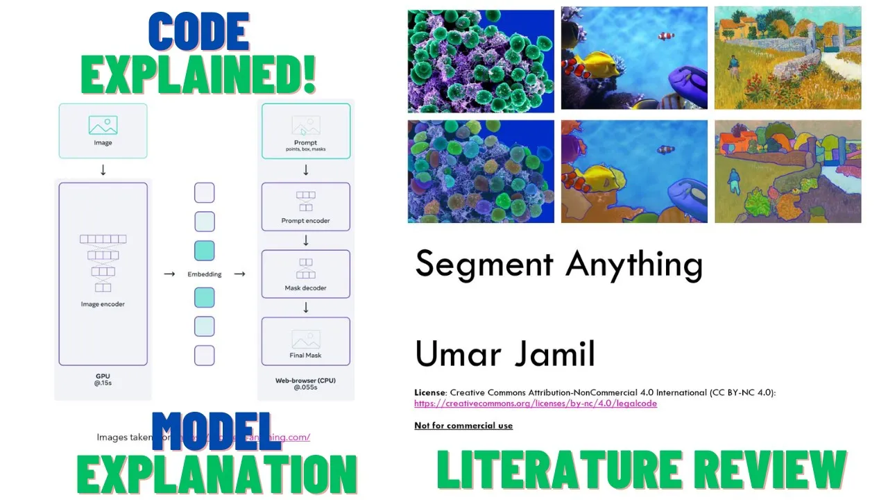
And in the best case, of course, all of them. Now let's overview the model. What is the model architecture? The model, as we saw before, is an encoder-decoder model. And it's composed of these parts. There is an image encoder that creates an embedding, given an image creates an embedding.

Then we have a prompt encoder that can encode the prompts given by the user, which can be points, boxes, text, or a combination. Then we will see later what is this mask here, but basically it means that if we run the model with an initial prompt, for example, a single point, the model will build an initial mask.

Then if we want to modify our prompt by adding another point, we can, instead of letting the model guess what we want, we can reuse the previous output to guide the model into telling the model that, okay, the previous mask was good, but not perfect. So I am giving you, again, the previous mask as a hint, as a starting point, plus some few points to guide you into telling you what I want you to remove or add to the mask.

This is the whole idea of this mask we can see here. So it's a mask, is the result of a previous prompting of this model. And then the model has a decoder that is given the prompt, the previous mask, and the embedding of the image, it has to predict the mask along with the scores of confidence score.

Now let's go and watch what is the image encoder and how does it work? In the paper, they say that they use the MAE pre-trained vision transformer. So MAE means that it's a masked autoencoder and a vision transformer. So let's review these two terms, what they mean and how they work.

Let's first review the vision transformer. The vision transformer was introduced in a very famous paper, I think a few years ago. The paper name is "An image is worth 16 by 16 words" and it's from Google Research, Google Brain. Basically what they did is, they take a picture, in this case, this one, they divide it into patches of 16 by 16, and then they flatten these patches, so create a sequence of these patches.

For example, this is the first patch, this is the second one, this is the third one, the fourth, etc. And then they created embedding by using a linear projection. So the embedding that captures somehow the information from each of this patch. They feed all this sequence of patches and actually the embedding of these patches along with the position encoding to the transformer.

But they not only feed the list of patches, but also another token here that is prepended to this sequence of patches. And this token is called the class embedding, the class token. And the idea comes from the BERT paper. Basically if you remember the transformer, when we have a sequence in the transformer encoder, the transformer basically allows, with its self-attention mechanism, to relate the tokens to each other.

So in the output we will have again a sequence of tokens, but the embedding of each token will somehow capture the interaction of that token with all the other tokens. And this is the idea behind adding this class token we have here. So we send it to the transformer, and at the output of the transformer, as soon as we will get another sequence in the output of the transformer encoder, we just take the first token here, and we ask this token to map this token to a multilayer perceptron that has to predict the class.

Why do we use this token? Because this token, because of the self-attention mechanism, has interacted with all of the other patches. So this token somehow captures the information of the other patches, and then we force the model to convey all this information to this single token. So this is the idea of the vision transformer and of the class token.

They took the vision transformer and they transformed it into a masked autoencoder vision transformer. And this happened in another paper called Masked Autoencoders are Scalable Vision Learners from Facebook, from Meta. Now in this case they still have an input image, in this case this one, but what they did is they split it into patches, but then they masked it out, they deleted some patches and replaced it with zeros, so they hide some patches here, and if I remember correctly it's 75% of the patches are masked out.

Then they only take the visible patches, create a sequence, a linear sequence here, they give it to the encoder of a transformer, which still produces as output a sequence as we saw before. Then what they do, they take this sequence that is the output of the encoder of the transformer, they again recreate the original image sequence, so if we knew that the first patch was empty, then they put an empty space here, then an empty, then the third one was visible, so they used the first embedding.

Then the fourth, the fifth and the sixth were deleted, so four, five and six were deleted, then they take the next one visible and they put it here. So basically to the decoder they give the visible patches and the non-visible patches along with the geometric information of the visibility.

So they are added in the same sequence in which they were cancelled out in the original image, and then they ask the decoder to predict the original image, only being able to visualize the embedding of the visible patches. So basically the decoder has to come up with a full image, being only able to access 25% of the image.

And what they saw is that the decoder was actually able to rebuild the original image, maybe not with the perfect quality, but a reasonable quality. And what the authors of the segment editing paper did, they took this part of the masked autoencoder of the vision transformer, because they are interested in this, the embedding learned by the encoder, so the output of the encoder.

Because if the model is able to predict the original image, given only this embedding of the visible patches, it means that these embeddings capture most of the information of the image, which can be then reused to rebuild the original image. So this is what they want, but this is what we want from an encoder.

We want the encoder to create a representation of something that captures most of its salient information without caring about the extra information that is not necessary. So this allows you to reduce the dimensionality of the original image while preserving the information. And this is why they use the encoder of the masked autoencoder vision transformer.

Now that we have seen what is the image encoder, which is basically creating an embedding, this one here, now we go to the next part, which is the prompt encoder. So the job of the prompt encoder is also to encode the prompt, which is the list of points chosen by the user, the boxes selected by the user and the text.

We will not visualize what is the text encoder, which is basically just the encoder of the clip model. So if you are not familiar with the clip model, I suggest you watch my previous video about the clip model, and it's quite interesting, actually, it's per se, so it deserves its own video.

But basically the idea is the same as with the image encoder. So we have a text and we want some representation that captures most of the information about this text. And this is done by the encoder of the clip text encoder. Let's have a look at the prompt encoder now.

Now in the prompt in their paper, segment anything, they say that they consider two type of prompts, the sparse prompts, which is the points, boxes and text, and the dense prompts, which is the mask we saw before. For the text encoder, they just use the text encoder from clip, we can see here, while the other two prompts, so the points and the boxes are basically they take the points, they create a representation of this point.

So an embedding that tells the model what is this point referring to inside of the image using the positional encoding. Let's see how does it work on a code level. Here we can see that basically, they take the sparse prompts, and they are mapped to 256 dimensional vector embeddings.

So 256 dimensional vector embeddings. Basically here is how we encode the points. We have the points, and then we have labels. The points are a sequence of X and Ys, while the labels indicate if the point is additive, so we want the model to add something to our mask, or subtractive, we want the model to remove something.

Here they are called foreground or background. Foreground means that we want the model to add something, background we want the model to remove something, just like we did with the example on the website before. So the first thing they do is they create the positional encoding of these points.

So they convert the X and the Y into positional encodings, exactly like we do in the transformer model. As you remember in the transformer model we have positional encodings. They are special vectors that tell the model, that are combined with the embedding of each token to tell the model what is the position of the token inside of the sentence.

And here the idea is the same, even if the positional encodings are different. I mean the idea is the same, so that it's a vector with the dimension 256, but they are built in a different way, and we will see why. But we have to think that they transform the X and the Y into vectors, each of them representing the position of the point inside of the image using the positional encoding.

Then they need to tell the model what is this point. The model cannot know if that point is foreground or background. So how do we do that? Basically all the foreground points are summed to another embedding here. That indicates it's an embedding that indicates that that is a foreground point.

And all the background points are summed to another embedding that indicates to the model that that point is a background point. And if the point is a padding, because we don't have enough points, then they use another special embedding here. And this is how they build the embedding for the points.

While for the boxes, the boxes are defined using the top left corner, so X and Y of the top left corner, and the bottom right corner. And they do the same with the boxes. So basically they transform these two points, so the top left and the bottom right, using the positional encodings to tell the model what is that X and Y corresponding to inside of the image.

And then they sum one embedding to indicate that it's a top left point and another embedding to indicate that it's a bottom right point. And this is how they build the encoding for the prompt. Why do we want to create 256 dimensional vector embeddings? Because the 266 dimension is also the one used for the image embedding.

Because then we can combine them using a transformer. So the mask we saw before, what is the role of the mask? Now let's go into the detail of how it's combined with the image. So basically, the masks are called a dense prompt in the segment editing model. And what they do is, if the mask is specified, so here, okay, if the mask is specified, basically they run it through a sequence of layers of convolutions to downscale this mask.

And then if no mask is specified, they create a special embedding called no mask. And it's defined here. So as you can see, it's just an embedding with a given dimension. How they combine this mask with the image, they just use a pointwise sum, as you can see here.

So they take the image and they just add the dense prompt embeddings, which is the mask embeddings. Now, as we saw before, we have to use the positional encoding to tell the model what are the points that we are feeding to the model itself. So the model cannot know X and Y, the model has need to know some other information.

We cannot just feed a list of X and Y to the model. We need to tell the model something more, something that can be learned by the model. And since the transformer models were very good at detecting the position using the sinusoidal positional encoding using the vanilla transformer. So if you remember in the vanilla transformer, so the transformer that was introduced in the paper, attention is all you need, if you remember, the positional encodings were built using sinusoidal functions.

So sines and cosines combined together. And these vectors told the model what is the position of the token inside of the sentence. Now, this was fine as long as we worked with text, because text only move along one dimension, that is, we have the token number zero, the token number one, the token number two, etc.

But pixels don't move in one direction, they move into two directions. So one person, of course, one could think, why not use the one positional encoding for the X coordinate to convert the X coordinate into a vector and another to map the Y coordinate into a vector? Yeah, we could do this.

But the problem is, if we do in this way, suppose we convert the center position of the image into two vectors, one encoded using the X coordinate and one encoded using the Y coordinate. What we do if we check the similarity with the other position in the image is we get some hitmap like this, in which the zero, this position here is very similar to this position here.

But it's not similar to this position here, which is not good, because in the in an image, we have the Euclidean distance. So pixel at the same Euclidean distance should have similarity with another point at the same distance. So basically, this point and this point should have a similarity that is the same as this point and this point.

Because we have a spatial representation, so pixels that are close to each other should be very similar, pixels that are far from each other should not be very similar. But this is not what happens in this hitmap. What we want is something like this, that is, if we have a point here, all the points in the radius of, let's say, 10 pixels are very similar.

All the points in the radius of 20, so distance 20, are less similar, but still, depending on the radius, they are similar in the same way as the other points with the same radius. And the more we go far from the center, the more we become distant, the more we become different.

And this is what we want from positional encodings for an image. And this idea was introduced in this paper. You can see learnable Fourier features from multidimensional spatial positional encoding. And however, this is not the paper used by Segment Anything. For Segment Anything, they use this paper here, but you understood why we needed a new kind of positional encoding.

Basically because we need to map two-dimensional mapping of X and Y to... we need to give an X and Y mapping to the model. We cannot just give them independent. And now let's look at the most important part of the model, which is the decoder. Now before we look at the decoder, I want to remind you that in the model that we saw before on the web browser, we could add the points on the real time in the browser.

That is, we loaded the image, and then I clicked on the model, and basically after a few milliseconds, let's say 100 milliseconds or half a second, I saw the output of the model. This could happen because the decoder is very fast, and the prompt encoder is very fast. But the image encoder doesn't have to be very fast, because we only encode the image once when we load the image.

Then we can do multiple prompts, so we can save the image embeddings, and then we just change the prompt embeddings and run them through the decoder to get the new masks. Which means basically that the image encoder can be powerful, even if it's slow, but the mask decoder has to be lightweight and fast.

And the same goes for the prompt encoder, and this is actually the case, because that's why we could use it on my browser in a reasonable time. So the mask decoder is made in this way. It's made of two layers, so we have to think that there is this block here, is repeated again with another block that is after this one, where the output of this big block is fed to the other block, and the output of that block is actually sent to the model here.

Let me delete that. Okay. Now let's look at the input of this decoder. First of all, we have the prompts here. So the prompts sent by the user, so the clicks, the boxes, and then we have the image embedding plus the mask we can see in the picture here.

So the image has already been combined with the mask through this layer here, through this addition, element-wise addition. The first thing the model, the decoder does is the self-attention. So the self-attention between the prompt tokens and with the prompt tokens. But here we can also see that there are these output tokens.

So before we proceed to see these steps, let's watch what are the output tokens. The output tokens take the idea also from BERT. So as you remember before, we saw the vision transformer, right? In the vision transformer, when they fed the patches to the transformer encoder, they also prepended another token called the class.

And the same idea is reused by segment anything, in which they append some tokens before the promptable tokens, so the boxes, the clicks made by the user. And then at the output of this decoder, they check again only these tokens and force the model to put all the information into these tokens.

So in this case, we have one token that tells the IOU, so the intersection over union scores of the predicted masks. And we will see later what is the IOU, if you're not familiar with it. And then there are three mask tokens, so one token for each mask. And basically, we feed these four tokens, so one IOU and three masks to the model.

We take them here at the output. And then we use the first token, so the IOU token, before we map it to a multi-layer perceptron, to force the model to learn the IOU score into these tokens. And then the other three are used to predict the three masks as output.

And we can see that here, they use the idea just like in the BERT paper. And this is the reference to the BERT paper in which they introduced the CLS token, in which in BERT was used for classification tasks. So basically, also in BERT, they prepended this token called the CLS.

And then, at the output of the transformer, they just took the token corresponding to this CLS, which was the first one, and they forced the model to learn all the information it needed to classify into this CLS token. Why this works? Because the CLS token could interact with all the other tokens through the self-attention mechanism.

And the same idea is reused here. So we feed the model with output tokens combined with the PROM tokens. And you can see here, they just concatenate the two. They take the IOU token and the mask token, they concatenate together. And then they concatenate these output tokens with the PROM tokens you can see here.

Now the second part, they run attention. So first, they run the self-attention with the tokens, which are the output tokens plus the PROM tokens. And this part is here. You can see that the query, the key, and the values are the same. And they are the PROM tokens. The comments have been added by me, they are not present in the original code to make your life easier.

Even if I found it really hard to follow this nomenclature, because sometimes they use the name is called Q, but then they pass it as K or P, etc. But hopefully it's clear enough. What we want to get from this code is actually not the single instructions, but the overall concepts.

So the output of this self-attention is then fed to a cross-attention. What is a cross-attention? Basically, a cross-attention is an attention in which the query comes from one side, and the key and the value come from another side. If you remember my video about the transformer model, in a translation task usually, imagine we are translating from English to Italian, or English to French, or English to Chinese.

Basically, we first run in the encoder a self-attention between all the input sentence, so all the tokens of the input sentence related to all the other tokens of the input sentence. And then in the decoder, we have this cross-attention in which we take the queries coming from one language and the key and the values coming from another language.

And this is usually done to combine two different sequences, to relate two different sequences with each other. In this case, what we want is to relate the tokens, so our prompt, with the image embeddings. This is why we do a cross-attention. So the first cross-attention is the tokens used as queries, while the image embeddings are used as keys and values.

And this is the first cross-attention. Then there is a multilayer perceptron, so it's just linear layers. And finally, we have another cross-attention, but this time the opposite. So in this case, the queries are the image embeddings and the keys and the values are the prompt tokens. Why do we want two cross-attentions?

Because we want two outputs from this transformer. One will be the sequence of tokens of the prompt, from which we will extract the output tokens, one indicating the IOU score and three indicating the mask. And one is the image embedding that we will then combine with the output tokens of the mask to build the mask.

But we will see this later. Another thing here highlighted in the paper is that to ensure that the coder has critical geometric information, the positional encodings are added to the image embedding whenever they participate in an attention layer. And as you can see, this is done not only for the image, but also for the prompt.

So every time to the prompt, they add the positional encoding, and every time to the image embedding, they also add the positional encoding. Why do we keep adding them? Because we don't want to lose this information after all these layers. And this is usually done with a skip connection.

And in this case, they just add them back. And now let's have a look at the output. As we saw before, we have a special layer of tokens added to the input of the transformer. One is for the IOU prediction and three are for the mask prediction. And you can see them here.

Because our transformer model has two cross-attentions, we have two outputs, two sequences outputs. One is the output sequence of the tokens, and one is the output sequence of the embeddings of the image. And they extract the IOU token, which is the first token added to the sequence, and then they extract the mask tokens, which are the first three, skipping the first one, the next three tokens.

Then what they do? They give the IOU tokens, they just give it to a prediction head to predict the IOU scores, and we can see that here. And then they take the output tokens for the masks, we can see them here, and they combine them with the upscaled embedding of the image.

So they take the output of the transformer for the image, so SRC in this case, the variable name is SRC, they upscale it here, and then they run each of the mask output tokens through its own MLP layer. So here you can see we have multiple MLP blocks here.

Each of the tokens have its own MLP block. They run each of them through its own, they get the output, and then they combine this output of this MLP, one for each token, one for each mask, with the upscale embedding of the image to produce the output mask here.

Another interesting part of the paper is this section here, making the model ambiguity aware. So as I was saying before, we not only predict one mask, but we predict three masks. And this happens when we do not have more than one prompt. So if we only click one, for example, once, the model will produce three masks.

But if we have more than one prompt, because the ambiguity becomes less, at least theoretically, the authors decided to add a fourth token that predicts another mask that is used only when we have more than one prompt. And this mask is never returned for the single prompt. Now let's have a look at what is intersection over union.

Intersection over union allows us to understand how good is our prediction given the ground truth, especially in segmentation models or object detection models. So for example, imagine we are using object detection and our ground truth box is this green box here, but our object, our model produced this red prediction as output.

So because you can see that even if there is some overlapping, but it doesn't cover the entire image, the prediction is quite poor. But this improves when the box becomes bigger. So the red box becomes bigger. So there is more intersection, but also more union. And finally, it becomes excellent when the intersection is covering all the box and it's covering all the union.

So the union of the two, basically the same box and they cover as most as possible. This area here, so the area that is predicted, but was not asked in the ground truth is called false. This one here is called false positive, while the area that should have been predicted, but was not predicted is called false negative.

This is a commonly used term also in this kind of scenarios. Now let's have a look at the loss. The loss of the model is a combination of two loss. One is called the focal loss and one is the dice loss, and they are used in a ratio of 20 to one.

Let's have a look at the focal loss. The focal loss takes his idea from the cross entropy, but with a modification that is the focal loss is adjusted for class imbalance. So why do we have a class imbalance in this case? Because imagine we are using a segmentation. We are trying to predict the map, the mask for a particular object in our image.

But of course, usually the mask is not covering the entire image, but it's only very few pixels compared to the total image are actually participating in this mask. And the instances of big mask are actually not so many. So we have a class imbalance here because most of our pixel will be non mask and only a small percentage of our pixel will be mask.

So we cannot use cross entropy in this case because the cross entropy doesn't pay attention to this class imbalance. So this is why they use focal loss to pay attention to this class imbalance. But the focal loss derives from the cross entropy and it was introduced in this paper by Facebook research, you can see here focal loss for dense object detection.

The next loss is the dice loss. The dice loss comes from the Soren dice coefficient and it's also called the F1 score. And it's calculated as the total to twice the intersection. So twice the area of overlap divided by the total area. And this is the actually a measure of similarity of between two sets of data.

To get the loss, we just do one minus the dice score. If you want more information about this dice score, which is very commonly used, I suggest you click on this link. It's on Medium. It's a nice article on how it works. And the dice loss was introduced in this paper VNet, I think it's from 2015.

Another interesting thing is that a segment anything built its own data set. And this is remarkable because we saw before that the segment anything has been trained on 1.1 billion masks using millions of images. And the data engine that was used to build this data set of 1.1 billion mask is composed of three stages.

The first one was a manual stage, then a semi automatic stage and then a fully automatic stage. Let's review them. In the assisted manual stage, so the manual stage, basically they hired a team of professional annotators that manually labeled the images using only the brush and the eraser tool.

So basically you have to think that there are many people who are using only pixel by pixel mapping this pixel to masks. So this is what we would do to create a data set from zero. Then they train this model on this manually created masks. And then they went to the semi automatic stage, that is, some of the masks were already generated by our model, which was trained on the manually generated mask.

And then the operators only had to adjust this mask to annotate any additional annotated objects that were missed from the model. And finally, this create even more samples and they train the model on this sample. And finally, they created the fully automatic stage. In this fully automatic stage, the model, there is no operator.

The model is building the data set by itself. How does it do? They take an image, they create a grid of 32 by 32 points. And then for each of these points, they ask the model to predict the masks. Of course, this will produce a lot, a large number of masks.

So they only take the one with the highest confidence score and also the only one that are stable. And by stable, they mean that if they threshold the probability map at 0.5 minus delta and 0.5 plus delta, they result in similar masks. Next, because we have a lot of masks and some of them may be overlapping with each other, some of them may be duplicate, actually, we need to remove some of them.

So we use an algorithm called the non-maximal suppression. This is very famous also in object detection. Let's review how it works. So non-maximal suppression usually works like this. Imagine we have an object detection model. Usually when we detect a bounding box for an object, we get a lot of bounding boxes.

And how do we only select one? Well, basically, we take the one with the highest confidence score, and then we delete all the other bounding boxes that have an IOU threshold with the one that we selected higher than one threshold that is given as parameter. This allow us to eliminate all the bounding boxes that are similar to the one we have selected.

And which one did we select? The one with the highest score. And then we do this for all the remaining boxes. And the algorithm is very simple, and it's also very effective. Thank you guys for watching my video about the segment anything. I hope that most of the information was clear.

If not, please let me know in the comments. I will try to complement my errors or some misunderstanding or something that I should have said better. I please subscribe to my channel because I will be uploading more videos in the future. And hopefully see you again.