So one of the things I wanted to talk about and it really came up when I was looking at the survey responses is what is different about how we're trying to teach this course and how will it impact you as participants in this course. And really we're trying to teach this course in a very different way to the way most teaching is done, or at least most teaching in the United States.

Rachel and I are both very keen fans of this guy called David Perkins who has this wonderful book called Making Learning Whole, How Seven Principles of Teaching Can Transform Education. We are trying to put these principles in practice in this course. I'll give you a little anecdote to give you a sense of how this works.

It's an anecdote from the book. If you were to learn baseball, if you were to learn baseball the way that math is taught, you would first of all learn about the shape of a parabola, and then you would learn about the material science design behind stitching baseballs and so forth.

And 20 years later after you had completed your PhD in postdoc, you would be taken to your first baseball game and you would be introduced to the rules of baseball, and then 10 years later you might get to here. The way that in practice baseball is taught is we take a kid down to the baseball diamond and we say these people are playing baseball.

Would you like to play it? And they say, "Yeah, sure I would." You say, "Okay, stand here, I'm going to throw this, hit it." Okay, great. Now run. Good. You're playing baseball. So that's why we started our first class with here are 7 lines of code you can run to do deep learning.

Not just to do deep learning, but to do image classification on any data set as long as you structure it in the right way. So this means you will very often be in a situation, and we've heard a lot of your questions about this during the week, of gosh there's a whole lot of details I don't understand.

Like this fine-tuning thing, what is fine-tuning? And the answer is we haven't told you yet. It's a thing you do in order to do effective image classification with deep learning. We're going to start at the top and gradually working our way down and down and down. The reason that you are going to want to learn the additional levels of detail is so that when you get to the point where you want to do something that no one's done before, you'll know how to go into that detail and create something that does what you want.

So we're going to keep going down a level and down a level and down a level and down a level, but through the hierarchy of software libraries, through the hierarchy of the way computers work, through the hierarchy of the algorithms and the math. But only at the speed that's necessary to get to the next level of let's make a better model or let's make a model that can do something we couldn't do before.

Those will always be our goals. So it's very different to, I don't know if anybody has been reading the Yoshua Bengio and Ian Goodfellow deep learning book, which is a great mathematical deep learning book, but it literally starts with 5 chapters of everything you need to know about probability, everything you need to know about calculus, everything you need to know about linear algebra, everything you need to know about optimization and so forth.

And in fact, I don't know that in the whole book there's ever actually a point where it says here is how you do deep learning, even if you read the whole thing. I've read 2/3 of it before, it's a really good math book. And anybody who's interested in understanding the math of deep learning I would strongly recommend but it's kind of the opposite of how we're teaching this course.

So if you often find yourself thinking, "I don't really know what's going on," that's fine. But I also want you to always be thinking about, "Well how can I figure out a bit more about what's going on?" So we're trying to let you experiment. So generally speaking, the assignments during the week are trying to give you enough room to find a way to dig into what you've learned and learn a little bit more.

Make sure you can do what you've seen and also that you can learn a little bit more about it. So you are all coders, and therefore you are all expected to look at that first notebook and look at what are the inputs to every one of those cells? What are the outputs from every one of those cells?

How is it that the output of this cell can be used as the input of that cell? Why is this transformation going on? This is why we did not tell you how do you use Kaggle CLI? How do you prepare a submission in the correct format? Because we wanted you to see if you can figure it out and also to leverage the community that we have to ask questions when you're stuck.

Being stuck and failing is terrific because it means you have found some limit of your knowledge or your current expertise. You can then think really hard, read lots of documentation, and ask the rest of the community until you are no longer stuck, at which point you now know something that you didn't know before.

So that's the goal. Asking for help is a key part of this, and so there is a whole wiki page called How to Ask for Help. It's really important, and so far I would say about half the times I've seen people ask for help, there is not enough information for your colleagues to actually help you effectively.

So when people point you at this page, it's not because they're trying to be a pain, it's because they're saying, "I want to help you, but you haven't given me enough information." So in particular, what have you tried so far? What did you expect to happen? What actually happened?

What do you think might be going wrong? What if you tried to test this out? And tell us everything you can about your computer and your software. Yes, Rachel? Where you've looked so far? Show us screenshots, error messages, show us your code. So the better you get at asking for help, the more enjoyable experience you're going to have because continually you'll find your problems will be solved very quickly and you can move on.

There was a terrific recommendation from the head of Google Brain, Vincent van Hooke, on a Reddit AMA a few weeks ago where he said he tells everybody in his team, "If you're stuck, work at it yourself for half an hour. You have to work at it yourself for half an hour.

If you're still stuck, you have to ask for help from somebody else." The idea being that you are always making sure that you try everything you can, but you're also never wasting your time when somebody else can help you. I think that's a really good suggestion. So maybe you can think about this half an hour rule yourself.

I wanted to highlight a great example of a really successful how to ask for help. Who asked this particular question? This is really well done. So that was really nice. What's your background before being here at this class? You could introduce yourself real quick, please. Hey, I actually graduated from U.S.S.

two years ago with the Master of U.S.S. later in elements. So that's why it was taught us as a team back to this class. Well, hopefully you've heard some of these fantastic approaches to asking for help. You can see here that he explained what he's going to do, what happened last time, what error message you got.

We've got a screenshot showing what he typed and what came back. He showed us what resources he's currently used, what these resources say, and so forth. Do you get your own question answered? Yes. Okay, great. Thanks very much. Sorry. Good for you. Thank you for coming in. I'm so happy when I saw this question because it's just so clear.

I was like, this is easy to answer because it's a well-asked question. So as you might have noticed, the wiki is rapidly filling out with lots of great information. So please start exploring it. You'll see on the left-hand side there is a recent changes section. You can see every day, lots of people have been contributing to lots of things, so it's continually improving.

There's some great diagnostic sections. If you are trying to diagnose something which is not covered and you solve it, please add your solution to these diagnostic sections. One of the things I love seeing today was Tom, where's Tom? Maybe his remote. Actually I think he was remote, I think he joined his remote yesterday.

So he was asking a question about how fine-tuning works, and we talked a bit about the answers, and then he went ahead and created a very small little wiki page. There's not much information there, but there's more than there used to be. And this is exactly what we want.

And you can even see in the places where he wasn't quite sure, he put some question marks. So now somebody else can go back, edit his wiki page, and Tom's going to come back tomorrow and say "Oh, now I've got even more questions answered." So this is the kind of approach where you're going to learn a lot.

We've already spoken to Melissa, so this is good. This is another great example of something which I think is very helpful, which is Melissa, who we heard from earlier, went ahead and told us all, "Here are my understanding of the 17 steps necessary to complete the things that we were asked to do this week." So this is great not only for Melissa to make sure she understands it correctly, but then everybody else can say "Oh, that's a really handy resource that we can draw on as well." There are 718 messages in Slack in a single channel.

That's way too much for you to expect to use this as a learning resource, so this is kind of my suggestion as to where you might want to be careful of how you use Slack. So I wanted to spend maybe quite a lot of time, as you can see, talking about the resources that are available.

I feel like if we get that sorted out now, then we're all going to speed along a lot more quickly. Thanks for your patience as we talk about some non-deep learning stuff. We expect the vast majority of learning to have an outside of class, and in fact if we go back and finish off our survey, I know that one of the questions asked about that.

How much time are you prepared to commit most weeks to this class? And the majority are 8-15, some are 15-30, and a small number are less than 8. Now if you're in the less than 8 group, I understand that's not something you can probably change. If you had more time, you'd put in more time.

So if you're in the less than 8 group, I guess just think about how you want to prioritize what you're getting out of this course, and be aware it's not really designed that you're going to be able to do everything in less than 8 hours a week. So maybe make more use of the forums and the wiki and kind of focus your assignments during the week on the stuff that you're most interested in.

And don't worry too much if you don't feel like you're getting everything, because you have less time available. For those of you in the 15-30 group, I really hope that you'll find that you're getting a huge amount of that time that you're putting in. Something I'm really glad I asked, because I found this very helpful, was how much was new to you?

And for half of you, the answer is most of it. And for well over half of you, most of it or nearly all of it from Lesson 1 is new. So if you're one of the many people I've spoken to during the week who are saying "holy shit, that was a fire hose of information, I feel kind of overwhelmed, but kind of excited.

You are amongst friends." Remember during the week, there are about 100 of you going through this same journey. So if you want to catch up with some people during the week and have a coffee to talk more about the class, or join a study group here at USF, or if you're from the South Bay, find some people from the South Bay, I would strongly suggest doing that.

So for example, if you're in Menlo Park, you could create a Menlo Park Slack channel and put out a message saying "Hey, anybody else in Menlo Park available on Wednesday night, I'd love to get together and maybe do some pair programming." For some of you, not very much of it was new.

And so for those of you, I do want to make sure that you feel comfortable pushing ahead, trying out your own projects and so forth. Basically in the last lesson, what we learned was a pretty standard data science computing stack. So AWS, Jupyter Notebook, bit of NumPy, Bash, this is all stuff that regardless of what kind of data science you do, you're going to be seeing a lot more of if you stick in this area.

They're all very, very useful things, and those of you who have maybe spent some time in this field, you'll have seen most of it before. So that's to be expected. So hopefully that is some useful background. So last week we were really looking at the basic foundations, computing foundations necessary for data science more generally, and for deep learning more particularly.

This week we're going to do something very similar, but we're going to be looking at the key algorithmic pieces. So in particular, we're going to go back and say "Hey, what did we actually do last week? And why did that work? And how did that work?" For those of you who don't have much algorithmic background around machine learning, this is going to be the same fire hose of information as last week was for those of you who don't have so much software and Bash and AWS background.

So again, if there's a lot of information, don't worry, this is being recorded. There are all the resources during the week. And so the key thing is to come away with an understanding of what are the pieces being discussed. Why are those pieces important? What are they kind of doing, even if you don't understand the details?

So if at any point you're thinking "Okay, Jeremy's talking about activation functions, I have no idea what he just said about what an activation function is, or why I should care, please go on to the in-class Slack channel and probably @Rachel, @Rachel, I don't know what Jeremy's talking about at all, and then Rachel's got a microphone and she can let me know, or else put up your hand and I will give you the microphone and you can ask.

So I do want to make sure you guys feel very comfortable asking questions. I have done this class now once before because I did it for the Skype students last night. So I've heard a few of the questions already, so hopefully I can cover some things that are likely to come up.

Before we look at these kind of digging into what's going on, the first thing we're going to do is see how do we do the basic homework assignment from last week. So the basic homework assignment from last week was "Can you enter the Kaggle Dogs and Cats Redux Competition?" So how many of you managed to submit something to that competition and get some kind of result?

Okay, that's not bad, so maybe a third. So for those of you who haven't yet, keep trying during this week and use all of those resources I showed you to help you because now quite a few of your colleagues have done it successfully and therefore we can all help you.

And I will show you how I did it. Here is Redux. So the basic idea here is we had to download the data to a directory. So to do that, I just typed "kg download" after using the "kg config" command. Kg is part of the Kaggle CLI thing, and Kaggle CLI can be installed by typing "p install Kaggle CLI".

This works fine without any changes if you're using our AWS instances and setup scripts. In fact it works fine if you're using Anaconda pretty much anywhere. If you're not doing either of those two things, you may have found this step more challenging. But once it's installed, it's as simple as saying "kg config" with your username, password and competition name.

When you put in the competition name, you can find that out by just going to the Kaggle website and you'll see that when you go to the competition in the URL, it has here a name. Just copy and paste that, that's the competition then. Kaggle CLI is a script that somebody created in their spare time and didn't spend a lot of time on it.

There's no error handling, there's no checking, there's nothing. So for example, if you haven't gone to Kaggle and accepted the competition rules, then attempting to run Kg download will not give you an error. It will create a zip file that actually contains the contents of the Kaggle webpage saying please accept the competition rules.

So those of you that tried to unzip that and that said it's not a zip file, if you go ahead and cat that, you'll see it's not a zip file, it's an HTML file. This is pretty common with recent-ish data science tools and particularly with cutting HTML learning stuff.

A lot of it's pretty new, it's pretty rough, and you really have to expect to do a lot of debugging. It's very different to using Excel or Photoshop. When I said Kg download, I created a test.zip and a train.zip, so I went ahead and I unzipped both of those things, that created a test and a train, and they contained a whole bunch of files called cat.one.jpg and so forth.

So the next thing I did to make my life easier was I made a list of what I believed I had to do. I find life much easier with a to-do list. I thought I need to create a validation set, I need to create a sample, I need to move my cats into a cats directory and dogs into a docs directory, I then need to run the fine tune and train, I then need to submit.

So I just went ahead then and created markdown headings for each of those things and started filling them out. Create validation set and sample. A very handy thing in Jupyter, Jupyter Notebook, is that you can create a cell that starts with a % sign and that allows you to type what they call magic commands.

There are lots of magic commands that do all kinds of useful things, but they do include things like cd and makedir and so forth. Another cool thing you can do is you can use an explanation mark and then type any bash command. So the nice thing about doing this stuff in the notebook rather than in bash is you've got a record of everything you did.

So if you need to go back and do it again, you can. If you make a mistake, you can go back and figure it out. So this kind of reproducible research, very highly recommended. So I try to do everything in a single notebook so I can go back and fix the problems that I always make.

So here you can see I've gone into the directory, I've created my validation set, I then used three lines of Python to go ahead and grab all of the JPEG file names, create a random permutation of them, and so then the first 2000 of that random permutation are 2000 random files, and then I moved them into my validation directory, that gave them my valid.

I did exactly the same thing for my sample, but rather than moving them, I copied them. And then I did that for both my sample training and my sample validation, and that was enough to create my validation set and sample. The next thing I had to do was to move all my cats into a cats directory and dogs into a dogs directory, which was as complex as typing move cat.star cats and dogs.star dogs.

And so the cool thing is, now that I've done that, I can then just copy and paste the seven lines of code from our previous lesson. So these lines of code are totally unchanged. I added one more line of code which was save weights. Once you've trained something, it's a great idea to save the weights so you don't have to train it again, you can always go back later and say load weights.

So I now had a model which predicted cats and dogs through my Redux competition. My final step was to submit it to Kaggle. So Kaggle tells us exactly what they expect, and the way they do that is by showing us a sample of the submission file. And basically the sample shows us that they expect an ID column and a label column.

The ID is the file number, so if you have a look at the test set, you'll see everyone's got a number. So it's expecting to get the number of the file along with your probability. So you have to figure out how to take your model and create something of that form.

This is clearly something that you're going to be doing a lot. So once I figured out how to do it, I actually created a method to do it in one step. So I'm going to go and show you the method that I wrote. So I just added this utils module that I kind of chucked everything in.

Actually that's not true, I'll put it in my VGG module because I added it to the VGG class. So there's a few ways you could possibly do this. Basically you know that you've got a way of grabbing a mini-batch of data at a time, or a mini-batch of predictions at a time.

So one thing you could do would be to grab your mini-batch size 64, you could grab your 64 predictions and just keep appending them 64 at a time to an array until eventually you have your 12,500 test images all with a prediction in an array. That is actually a perfectly valid way to do it.

How many people solved it using that kind of approach? Not many of you, that's interesting, but it works perfectly well. Those of you who didn't, I guess either asked on the forum or read the documentation and discovered that there's a very handy thing in Keras called Predict Generator. And what Predict Generator does is it lets you send it in a bunch of batches, so something that we created with get_batches, and it will run the predictions on every one of those batches and return them all in a single array.

So that's what we wanted to do. If you read the Keras documentation, which you should do very often, you will find out that Predict Generator generally will give you the labels. So not the probabilities, but the labels, so cat1, dog0, something like that. In this case, for this competition, they told us they want probabilities, not labels.

So instead of calling the get_batches, which we wrote, here is the get_batches that we wrote, you can see all it's doing is calling something else, which is flow from directory. To get Predict Generator to give you probabilities instead of classes, you have to pass in an extra argument, which is plus mode equals, and rather than categorical, you have to say none.

So in my case, when I went ahead and actually modified get_batches to take an extra argument, which was plus mode, and then in my test method I created, I then added plus mode equals none. So then I could call model.PredictGenerator, passing in my batches, and that is going to give me everything I need.

So I will show you what that looks like. So once I do, I basically say vgg.test, this is the thing I created, pass in my test directory, pass in my batch size, that returns two things, it returns the predictions, and it returns the batches. I can then use batches.filenames to grab the filenames, because I need the filenames in order to grab the IDs.

And so that looks like this, let's take a look at them, so there's a few predictions, and let's look at a few filenames. Now one thing interesting is that at least for the first five, the probabilities are all 1's and 0's, rather than 0.6, 0.8, and so forth. We're going to talk about why that is in just a moment.

For now, it is what it is. It's not doing anything wrong, it really thinks that the answer. So all we need to do is grab, because Kaggle wants something which is is_dog, we just need to grab the second column of this, and the numbers from this, place them together as columns, and send them across.

So here is grabbing the first column from the predictions, and I call it is_dog. Here is grabbing from the 8th character until the dot in filenames, turning that into an integer, get my IDs. NumPy has something called stack, which lets you put two columns next to each other, and so here is my IDs and my probabilities.

And then NumPy lets you save that as a CSV file using save text. You can now either SSH to your AWS instance and use KgSubmit, or my preferred technique is to use a handy little IPython thing called FileLink. If you type FileLink and then pass in a file that is on your server, it gives you a little URL like this, which I can click on, and it downloads it to my computer.

And so now on my computer I can go to Kaggle and I can just submit it in the usual way. I prefer that because it lets me find out exactly if there's any error messages or anything going wrong on Kaggle, I can see what's happening. So as you can see, rerunning what we learned last time to submit something to Kaggle really just requires a little bit of coding to just create the submission file, a little bit of bash scripting to move things into the right place, and then rerunning the 7 lines of code, the actual deep learning itself is incredibly straightforward.

Now here's where it gets interesting. When I submitted my 1s and 0s to Kaggle, I was put in -- let's have a look at the leaderboard. The first thing I did was I accidentally put in "iscat" rather than "isdog", and that made me last place. So I had 38 was my loss.

Then when I was putting in 1s and 0s, I was in 110th place, which is still not that great. Now the funny thing was I was pretty confident that my model was doing well because the validation set for my model told me that my accuracy was 97.5%. I'm pretty confident that people on Kaggle are not all of them doing better than that.

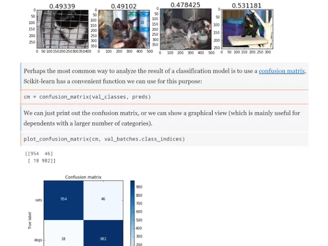
So I thought something weird is going on. So that's a good time to figure out what does this number mean? What is 12? What is 17? So let's go and find out. It says here that it is a log loss, so if we go to Evaluation, we can find out what log loss is.

And here is the definition of log loss. Log loss is known in Keras as binary entropy or categorical entropy, and you will actually find it very familiar because every single time we've been creating a model, we have been using -- let's go and find out when we compile it.

When we compile a model, we've always been using categorical cross-entropy. So it's probably a good time for us to find out what the hell this means. So the short answer is it is this mathematical function. But let's dig into this a little bit more and find out what's going on.

I would strongly recommend that when you want to understand how something works, you whip out a spreadsheet. Spreadsheets are like my favorite tool for doing small-scale data analysis. They are perhaps the least well-utilized tools among professional data scientists, which I find really surprising. Because back when I was in consulting, everybody used them for everything, and they were the most overused tools.

So what I've done here is I've gone ahead and created a little column of his cats and his dogs. So this is the correct answer, and I've created a little column of some possible predictions. And then I've just gone in and I've typed in the formula from that cattle page.

And so here it is. Basically it's the truth label times log of the prediction minus 1 minus the truth label times log of 1 minus the prediction. Now if you think about it, the truth label is always 1 or 0. So this is actually probably more easily understood using an if function.

It's exactly the same thing. Rather than multiplying by 1 and 0, let's just use the if function. Because if it's a cat, then take log of the prediction, otherwise take log of 1 minus the prediction. Now this is hopefully pretty intuitive. If it's a cat and your prediction is really high, then we're taking the log of that and getting a small number.

If it's not a cat and then our prediction is really low, then we want to take the log of 1 minus that. And so you can get a sense of it by looking here, here's like a non-cat, which we thought is a non-cat, and therefore we end up with log of 1 minus that, which is a low number.

Here's a cat, which we're pretty confident isn't a cat, so here is log of that. Notice this is all being a negative sign at the front just to make it so that smaller numbers are better. So this is log loss, or binary, or categorical cross-entropy. And this is where we find out what's going on.

Because I'm now going to go and try and say, well, what did I submit? And I've submitted predictions that were all 1s and 0s. So what if I submit 1s and 0s? Ouch. Okay, why is that happening? Because we're taking logs of 1s and 0s. That's no good. So actually, Kaggle has been pretty nice not to return just an error.

And I actually know why this happens because I wrote this functionality on Kaggle. Kaggle modifies it by a tiny 0.0001, just to make sure it doesn't die. So if you say 1, it actually treats it as 0.9999, if you say 0 it treats it as 0.0001. So our incredibly overconfident model is getting massively penalized for that overconfidence.

So what would be better to do would be instead of sending across 1s and 0s, why not send across actual probabilities you think are reasonable? So in my case, what I did was I added a line which was, I said numpy.clip, my first column of my predictions, and clip it to 0.05 and 0.95.

So anything less than 0.05 becomes 0.05 and anything greater than 0.95 becomes 0.95. And then I tried submitting that. And that moved me from 110th place to 40th place. And suddenly, I was in the top half. So the goal of this week was really try and get in the top half of this competition.

And that's all you had to do, was run a single epoch, and then realize that with this evaluation function, you need to be submitting things that aren't 1s and 0s. Let's take that one offline and talk about it in the forum because I actually need to think about that properly.

So probably I should have used, and I'll be interested in trying this tomorrow and maybe in a resubmission, I probably should have done 0.025 and 0.975 because I actually know that my accuracy on the validation set was 0.975. So that's probably the probability that I should have used. I would need to think about it more though to think like, because it's like a nonlinear loss function, is it better to underestimate how confident you are or overestimate how confident you are?

So I would need to think about it a little bit. In the end, I said it's about 97.5, I have a feeling that being overconfident might be a bad thing because of the shape of the function, so I'll just be a little bit on the tame side. I then later on tried 0.02 and 0.98, and I did actually get a slightly better answer.

I actually got a little bit better than that. I think in the end this afternoon I ran a couple more epochs just to see what would happen, and that got me to 24th. So I'll show you how you can get to 24th position, and it's incredibly simple. You take these two lines here, fit and save weights, and copy and paste them a bunch of times.

You can see I saved the weights under a different file name each time just so that I can always go back and use a model that I created earlier. Something we'll talk about more in the class later is this idea that halfway through after two epochs I changed my learning rate from 0.1 to 0.01 just because I happen to know this is often a good idea.

I haven't actually tried it without doing that. I suspect it might be just as good or even better, but that was just something I tried. So interestingly, by the time I run four epochs, my accuracy is 98.3%. That would have been second place in the original Cats and Dogs competition.

So you can see it doesn't take much to get really good results. And each one of these took, as you can see, 10 minutes to run on my AWS P2 instance. The original Cats and Dogs used a different evaluation function, which was just accuracy. So they changed it for the Redux one to use block loss, which makes it a bit more interesting.

The reason I didn't just say nb_epoch=4 is that I really wanted to save the result after each epoch under a different weights file name just in case at some point it overfit. I could always go back and use one that I got in the middle. We're going to learn a lot about that in the next couple of weeks.

In this case, we have added a single linear layer to the end. We're about to learn a lot about this. And so we actually are not training very many parameters. So my guess would be that in this case, we could probably run as many epochs as we like and it would probably keep getting better and better until it eventually levels off.

That would be my guess. So I wanted to talk about what are these probabilities. One way to do that, and also to talk about how can you make this model better, is any time I build a model and I think about how to make it better, my first step is to draw a picture.

Let's take that one offline onto the forum because we don't need to cover it today. Data scientists don't draw enough pictures. Now when I say draw pictures, I mean everything from printing out the first five lines of your array to see what it looks like to drawing complex plots.

For a computer vision, you can draw lots of pictures because we're classifying pictures. I've given you some tips here about what I think are super useful things to visualize. So when I wanted to find out how come my Kaggle submission is 110th place, I ran my kind of standard five steps.

The standard five steps are let's look at a few examples of images we got right, let's look at a few examples of images we got wrong. Let's look at some of the cats that we felt were the most cat-like, some of the dogs that we felt were the most dog-like, vice versa.

Some of the cats that we were the most wrong about, some of the dogs we were the most wrong about, and then finally some of the cats and dogs that our model is the most unsure about. This little bit of code I suggest you keep around somewhere because this is a super useful thing to do anytime you do image recognition.

So the first thing I did was I loaded my weights back up just to make sure that they were there and I took them from my very first epoch, and I used that vgg.test method that I just showed you that I created. This time I passed in the validation set, not the test set because the validation set I know the correct answer.

So then from the batches I could get the correct labels and I could get the file names. I then grabbed the probabilities and the class predictions, and that then allowed me to do the 5 things I just mentioned. So here's number 1, a few correct labels at random. So numpy.where, the prediction is equal to the label.

Let's then get a random permutation and grab the first 4 and plot them by index. So here are 4 examples of things that we got right. And not surprisingly, this cat looks like a cat and this dog looks like a dog. Here are 4 things we got wrong. And so that's interesting.

You can kind of see here's a very black underexposed thing on a bright background. Here is something that is on a totally unusual angle. And here is something that's so curled up you can't see its face. And this one you can't see its face either. So this gives me a sense of like, okay, the things that's getting wrong, it's reasonable to get those things wrong.

If you looked at this and they were really obvious, cats and dogs, you would think there's something wrong with your model. But in this case, no, the things that it's finding hard are genuinely hard. Here are some cats that we felt very sure were cats. Here are some dogs we felt very sure were dogs.

So these weights, this one here results ft1.h5, this ft stands for fine-tune, and you can see here I saved my weights after I did my fine-tuning. So these are the cats and dogs. So these I think are the most interesting, which is here are the images we were very confident were cats, but they're actually dogs.

Here's one that is only 50x60 pixels, that's very difficult. Here's one that's almost totally in front of a person and is also standing upright. That's difficult because it's unusual. This one is very white and is totally from the front, that's quite difficult. And this one I'm guessing the color of the floor and the color of the fur are nearly identical.

So again, this makes sense, these do look genuinely difficult. So if we want to do really well in this competition, we might start to think about should we start building some models of very very small images because we now know that sometimes cable gives us 50x50 images, which are going to be very difficult for us to deal with.

Here are some pictures that we were very confident are dogs, but they're actually cats. Again, not being able to see the face seems like a common problem. And then finally, here are some examples that we were most uncertain about. Now notice that the most uncertain are still not very uncertain, like they're still nearly one or nearly zero.

So why is that? Well, we will learn in a moment about exactly what is going on from a mathematical point of view when we calculate these things, but the short answer is the probabilities that come out of a deep learning network are not probabilities in any statistical sense of the term.

So this is not actually saying that there is one chance that I had of 100,000, that this is a dog. It's only a probability from the mathematical point of view, and in math the probability means it's between 0 and 1, and all of the possibilities add up to 1.

It's not a probability in the sense that this is actually something that tells you how often this is going to be right versus this is going to be wrong. So for now, just be aware of that. When we talk about these probabilities that come out of neural network training, you can't interpret them in any kind of intuitive way.

We will learn about how to create better probabilities down the track. Every time you do another epoch, your network is going to get more and more confident. This is why when I loaded the weights, I loaded the weights from the very first epoch. If I had loaded the weights from the last epoch, they all would have been 1 and 0.

So this is just something to be aware of. So hopefully you can all go back and get great results on the Kaggle competition. Even though I'm going to share all this, you will learn a lot more by trying to do it yourself, and only referring to this when and if you're stuck.

And if you do get stuck, rather than copying and pasting my code, find out what I used and then go to the Keras documentation and read about it and then try and write that line of code without looking at mine. So the more you can do that, the more you'll think, "Okay, I can do this.

I understand how to do this myself." Just some suggestions, it's entirely up to you. So let's move on. So now that we know how to do this, I wanted to show you one other thing, which is the last part of the homework was redo this on a different dataset.

And so I decided to grab the State Farm Distracted Driver Competition. The Kaggle State Farm Distracted Driver Competition has pictures of people in 10 different types of distracted driving, ranging from drinking coffee to changing the radio station. I wanted to show you how I entered this competition. It took me a quarter of an hour to enter the competition, and all I did was I duplicated my Cats and Dogs Redux notebook, and then I started basically rerunning everything.

But in this case, it was even easier because when you download the State Farm Competition data, they had already put it into directories, one for each type of distracted driving. So I was delighted to discover, let's go to it, so if I type "tree-d", that shows you my directory structure, you can see in "train", it already had 10 directories, it actually didn't have valid, so in "train", it already had the 10 directories.

So I could skip that whole section. So I only had to create the validation and sample set. If all I wanted to do was enter the competition, I wouldn't even have had to have done that. So I won't go through, but it's basically exactly the same code as I had before to create my validation set and sample.

I deleted all of the bits which moved things into separate subfolders, I then used exactly the same 7 lines of code as before, and that was basically done. I'm not getting good accuracy yet, I don't know why, so I'm going to have to figure out what's going on with this.

But as you can see, this general approach works for any kind of image classification. There's nothing specific about cats and dogs, so you now have a very general tool in your toolbox. And all of the stuff I showed you about visualizing the errors and stuff, you can use all that as well.

So maybe when you're done, you could try this as well. Yes, you know, can I grab one of these please? So the question is, would this work for CT scans and cancer? And I can tell you that the answer is yes, because I've done it. So my previous company I created was something called Enlidic, which was the first deep learning for medical diagnostics company.

And the first thing I did with four of my staff was we downloaded the National Lung Screening Trial data, which is a thousand examples of people with cancer, it's a CT scan of their lungs and 5,000 examples of people without cancer, CT scans of their lungs. We did the same thing.

We took ImageNet, we fine-tuned ImageNet, but in this case instead of cats and dogs, we had malignant tumor versus non-malignant tumor. We then took the result of that and saw how accurate it was, and we discovered that it was more accurate than a panel of four of the world's best radiologists.

And that ended up getting covered on TV on CNN. So making major breakthroughs in domains is not necessarily technically that challenging. The technical challenges in this case were really about dealing with the fact that CT scans are pretty big, so we had to just think about some resource issues.

Also they're black and white, so we had to think about how do we change our ImageNet pre-training to black and white, and stuff like that. But the basic example was really not much more of a different code to what you see here. The State Farm data is 4GB, and I only downloaded it like half an hour before class started.

So I only ran a small fraction of an epoch just to make sure that it works. I'm running a whole epoch, probably would have taken overnight. So let's go back to lesson 1, and there was a little bit at the end that we didn't look at. Actually before we do, now's a good time for a break.

So let's have a 12 minute break, let's come back at 8pm, and one thing that you may consider doing during those 12 minutes if you haven't done it already is to fill out the survey. I will place the survey URL back onto the in class page. See you in 12 minutes.

Okay thanks everybody. How many of you have watched this video? Okay, some of you haven't. You need to, because as I've mentioned a couple of times in our emails, the last two thirds of it was actually a surprise lesson 0 of this class, and it's where I teach about what convolutions are.

So if you haven't watched it, please do. The first 20 minutes or so is more of a general background, but the rest is a discussion of exactly what convolutions are. For now, I'll try not to assume too much that you know what they are, the rest of it hopefully will be stand-alone anyway.

But I want to talk about fine-tuning, and I want to talk about why we do fine-tuning. Why do we start with an image network and then fine-tune it rather than just train our own network? And the reason why is that an image network has learned a hell of a lot of stuff about what the world looks like.

A guy called Matt Zeiler wrote this fantastic paper a few years ago in which he showed us what these networks learn. And in fact, the year after he wrote this paper, he went on to win ImageNet. So this is a powerful example of why spending time thinking about visualizations is so helpful.

By spending time thinking about visualizing networks, he then realized what was wrong with the networks at the time, made them better and won the next year's ImageNet. We're not going to talk about that, we're going to talk about some of these pictures here, Drew. Here are 9 examples of what the very first layer of an ImageNet convolutional neural network looks like, what the filters look like.

And you can see here that, for example, here is a filter that learns to find a diagonal edge or a diagonal line. So you can see it's saying look for something where there's no pixels and then there's bright pixels and then there's no pixels, so that's finding a diagonal line.

Here's something that finds a diagonal line in the up direction. Here's something that finds a gradient horizontal from orange to blue. Here's one diagonal from orange to blue. As I said, these are just 9 of these filters in layer 1 of this ImageNet trained network. So what happens, those of you who have watched the video I just mentioned will be aware of this, is that each of these filters gets placed pixel by pixel or group of pixels by group of pixels over a photo, over an image, to find which parts of an image it matches.

So which parts have a diagonal line. And over here it shows 9 examples of little bits of actual ImageNet images which match this first filter. So here are, as you can see, they all are little diagonal lines. So here are 9 examples which match the next filter, the diagonal lines in the opposite direction and so forth.

The filters in the very first layer of a deep learning network are very easy to visualize. This has happened for a long time, and we've always really known for a long time that this is what they look like. We also know, incidentally, that the human vision system is very similar.

The human vision system has filters that look much the same. To really answer the question of what are we talking about here, I would say watch the video. But the short answer is this is a 7x7 pixel patch which is slid over the image, one group of 7 pixels at a time, to find which 7x7 patches look like that.

And here is one example of a 7x7 patch that looks like that. So for example, this gradient, here are some examples of 7x7 patches that look like that. So we know the human vision system actually looks for very similar kinds of things. These kinds of things that they look for are called Gabor filters.

If you want to Google for Gabor filters, you can see some examples. It's a little bit harder to visualize what the second layer of a neural net looks like, but Zyla figured out a way to do it. In his paper, he shows us a number of examples of the second layer of his ImageNet trained neural network.

Suppose we can't directly visualize them, instead we have to show examples of what the filter can look like. So here is an example of a filter which clearly tends to pick up corners. So in other words, it's taking the straight lines from the previous layer and combining them to find corners.

There's another one which is learning to find circles, and another one which is learning to find curves. So you can see here are 9 examples from actual pictures on ImageNet, which actually did get heavily activated by this corner filter. And here are some that got heavily activated by this circle filter.

The third layer then can take these filters and combine them, and remember this is just 16 out of 100 which are actually in the ImageNet architecture. So in layer 3, we can combine all of those to create even more sophisticated filters. In layer 3, there's a filter which can find repeating geometrical patterns.

Here's a filter, let's go look at the examples. That's interesting, it's finding pieces of text. And here's something which is finding edges of natural things like fur and plants. Layer 4 is finding certain kinds of dog face. Layer 5 is finding the eyeballs of birds and reptiles and so forth.

So there are 16 layers in our VGG network. What we do when we fine-tune is we say let's keep all of these learnt filters and use them and then just learn how to combine the most complex subtle nuanced filters to find cats versus dogs rather than combine them to learn a thousand categories of ImageNet.

This is why we do fine-tuning. So when I asked Yannette's earlier question about does this work for CT scans and lung cancer, and the answer was yes. These kinds of filters that find dog faces are not very helpful for looking at a CT scan and looking for cancer, but these earlier ones that can recognize repeating images or corners or curves certainly are.

So really regardless of what computer vision work you're doing, starting with some kind of pre-trained network is almost certainly a good idea because at some level that pre-trained network has learnt to find some kinds of features that are going to be useful to you. And so if you start from scratch you have to learn them from scratch.

In cats versus dogs we only had 25,000 pictures. And so from 25,000 pictures to learn this whole hierarchy of geometric and semantic structures would have been very difficult. So let's not learn it, let's use one that's already been learned on ImageNet which is one and a half million pictures.

So that's the short answer to the question "Why do fine-tuning?" To the longer answer really requires answering the question "What exactly is fine-tuning?" And to answer the question "What exactly is fine-tuning?" we have to answer the question "What exactly is a neural network?" So a neural network, we'll learn more about this shortly, but the short answer is if you're not sure, try all of it.

Generally speaking, if you're doing something with natural images, the second to last layer is very likely to be the best, but I just tend to try a few. And we're going to see today or next week some ways that we can actually experiment with that question. So as per usual, in order to learn about something we will use Excel.

And here is a deep neural network in Excel. Rather than having a picture with lots of pixels, I just have three inputs, a single row with three inputs which are x1, x2 and x3, and the numbers are 2, 3 and 1. And rather than trying to pick out whether it's a dog or a cat, we're going to assume there are two outputs, 5 and 6.

So here's like a single row that we're feeding into a deep neural network. So what is a deep neural network? A deep neural network basically is a bunch of matrix products. So what I've done here is I've created a bunch of random numbers. They are normally distributed random numbers, and this is the standard deviation that I'm using for my normal distribution, and I'm using 0 as the mean.

So here's a bunch of random numbers. What if I then take my input vector and matrix multiply them by my random weights? And here it is. So here's matrix multiply, that by that. And here's the answer I get. So for example, 24.03 = 2 x 11.07 + 3 x -2.81 + 1 x 10.31 and so forth.

Any of you who are either not familiar with or are a little shaky on your matrix vector products, tomorrow please go to the Khan Academy website and look for Linear Algebra and watch the videos about matrix vector products. They are very, very, very simple, but you also need to understand them very, very, very intuitively, comfortably, just like you understand plus and times in regular algebra.

I really want you to get to that level of comfort with linear algebra because this is the basic operation we're doing again and again. So if that is a single layer, how do we turn that into multi-layers? Well, not surprisingly, we create another bunch of weights. And now we take those weights, the new bunch of weights, times the previous activations with our matrix multiply, and we get a new set of activations.

And then we do it again. Let's create another bunch of weights and multiply them by our previous set of activations. Note that the number of columns in your weight matrix is, you can make it as big or as small as you like, as long as the last one has the same number of columns as your output.

So we have 2 outputs, 5 and 6. So our final weight matrix had to have 2 columns so that our final activations has 2 things. So with our random numbers, our activations are not very close to what we hope they would be, not surprisingly. So the basic idea here is that we now have to use some kind of optimization algorithm to repeatably make the weights a little bit better and a little bit better, and we will see how to do that in a moment.

But for now, hopefully you're all familiar with the idea that there is such a thing as an optimization algorithm. An optimization algorithm is something that takes some kind of output to some kind of mathematical function and finds the inputs to that function that makes the outputs as low as possible.

And in this case, the thing we would want to make as low as possible would be something like the sum of squared errors between the activations and the outputs. I want to point out something here, which is that when we stuck in these random numbers, the activations that came out, not only are they wrong, they're not even in the same general scale as the activations that we wanted.

So that's a bad problem. The reason it's a bad problem is because they're so much bigger than the scale that we were looking for. As we change these weights just a little bit, it's going to change the activations by a lot. And this makes it very hard to train.

In general, you want your neural network to start off even with random weights, to start off with activations which are all of similar scale to each other, and the output activations to be of similar scale to the output. For a very long time, nobody really knew how to do this.

And so for a very long time, people could not really train deep neural networks. It turns out that it is incredibly easy to do. And there is a whole body of work talking about neural network initializations. It turns out that a really simple and really effective neural network initialization is called Xavier initialization, named after its founder, Xavier Glauro.

And it is 2 divided by n+l. Like many things in deep learning, you will find this complex-looking thing like Xavier weight initialization scheme, and when you look into it, you will find it is something about this easy. This is about as complex as deep learning gets. So I am now going to go ahead and implement Xavier deep learning weight initialization schemes in Excel.

So I'm going to go up here and type =2 divided by 3in + 4out, and put that in brackets because we're complex and sophisticated mathematicians, and press enter. There we go. So now my first set of weights have that as its standard deviation. My second set of weights I actually have pointing at the same place, because they also have 4in and 3out.

And then my third I need to have =2 divided by 3in + 2out. Done! So I have now implemented it in Excel, and you can see that my activations are indeed of the right general scale. So generally speaking, you would normalize your inputs and outputs to be mean 0 and standard deviation 1.

And if you use these, we want them to be of the same kind of scale. Obviously they're not going to be in 5 and 6 because we haven't done any optimization yet, but we don't want them to be like 100,000. We want them to be somewhere around 5 and 6.

Eventually we want them to be close to 5 and 6. And so if we start off with them really high or really low, then optimization is going to be really finicky and really hard to do. And so for decades when people tried to train deep learning neural networks, the training that took forever or was so incredibly unresilient, it was useless, and this one thing, better weight initialization, was a huge step.

We're talking maybe 3 years ago that this was invented, so this is not like we're going back a long time, this is relatively recent. Now the good news is that Keras and pretty much any decent neural network library will handle your weight initialization for you. Until very recently they pretty much all used this.

There are some even more recent slightly better approaches, but they'll give you a set of weights where your outputs will generally have a reasonable scale. So what's not arbitrary is that you are given your input dimensionality. So in our case, for example, it would be 224x224 pixels, in this case I'm saying it's 3 things.

You are given your output dimensionality. So for example in our case, for cats and dogs it's 2, for this I'm saying it's 2. The thing in the middle about how many columns does each of your weight matrices have is entirely up to you. The more columns you add, the more complex your model, and we're going to learn a lot about that.

As Rachel said, this is all about your choice of architecture. So in my first one here I had 4 columns, and therefore I had 4 outputs. In my next one I had 3 columns, and therefore I had 3 outputs. In my final one I had 2 columns, and therefore I had 2 outputs, and that is the number of outputs that I wanted.

So this thing of like how many columns do you have in your weight matrix is where you get to decide how complex your model is, so we're going to see that. So let's go ahead and create a linear model. Alright, so we're going to learn how to create a linear model.

Let's first of all learn how to create a linear model from scratch, and this is something which we did in that original USF Data Institute launch video, but I'll just remind you. Without using Keras at all, I can define a line as being ax + b, I can then create some synthetic data.

So let's say I'm going to assume a is 3 and b is 8, create some random x's, and my y will then be my ax + b. So here are some x's and some y's that I've created, not surprisingly, this kind of plot looks like so. The job of somebody creating a linear model is to say I don't know what a and b is, how can we calculate them?

So let's forget that we know that they're 3 and 8, and say let's guess that they're -1 and 1, how can we make our guess better? And to make our guess better, we need a loss function. So the loss function is something which is a mathematical function that will be high if your guess is bad, and is low if it's good.

The loss function I'm using here is sum of squared errors, which is just my actual minus my prediction squared, and add it up. So if I define my loss function like that, and then I say my guesses are -1 and 1, I can then calculate my average loss and it's 9.

So my average loss with my random guesses is not very good. In order to create an optimizer, I need something that can make my weights a little bit better. If I have something that can make my weights a little bit better, I can just call it again and again and again.

That's actually very easy to do. If you know the derivative of your loss function with respect to your weights, then all you need to do is update your weights by the opposite of that. So remember, the derivative is the thing that says, as your weight changes, your output changes by this amount.

That's what the derivative is. In this case, we have y = ax + b, and then we have our loss function is actual minus predicted squared, then add it up. So we're now going to create a function called update, which is going to take our a guess and our b guess and make them a little bit better.

And to make them a little bit better, we calculate the derivative of our loss function with respect to b, and the derivative of our loss function with respect to a. How do we calculate those? We go to Wolfram Alpha and we enter in d along with our formula, and the thing we want to get the derivative of, and it tells us the answer.

So that's all I did, I went to Wolfram Alpha, found the correct derivative, pasted them in here. And so what this means is that this formula here tells me as I increase b by 1, my sum of squared errors will change by this amount. And this says as I change a by 1, my sum of squared errors will change by this amount.

So if I know that my loss function gets higher by 3 if I increase a by 1, then clearly I need to make a a little bit smaller, because if I make it a little bit smaller, my loss function will go down. So that's why our final step is to say take our guess and subtract from it our derivative times a little bit.

LR stands for learning rate, and as you can see I'm setting it to 0.01. How much is a little bit is something which people spend a lot of time thinking about and studying, and we will spend time talking about, but you can always trial and error to find a good learning rate.

When you use Keras, you will always need to tell it what learning rate you want to use, and that's something that you want the highest number you can get away with. We'll see more of this next week. But the important thing to realize here is that if we update our guess, minus equals our derivative times a little bit, our guess is going to be a little bit better because we know that going in the opposite direction makes the loss function a little bit lower.

So let's run those two things, where we've now got a function called update, which every time we run it makes our predictions a little bit better. So finally now, I'm basically doing a little animation here that says every time you calculate an animation, call my animate function, which 10 times will call my update function.

So let's see what happens when I animate that. There it is. So it starts with a really bad line, which is my -11, and it gets better and better. So this is how stochastic gradient descent works. Stochastic gradient descent is the most important algorithm in deep learning. Stochastic gradient descent is the thing that starts with random weights like this and ends with weights that do what you want to do.

So as you can see, stochastic gradient descent is incredibly simple and yet incredibly powerful because it can take any function and find the set of parameters that does exactly what we want to do with that function. And when that function is a deep learning neural network that becomes particularly powerful.

It has nothing to do with neural nets except - so just to remind ourselves about the setup for this, we started out by saying this spreadsheet is showing us a deep neural network with a bunch of random parameters. Can we come up with a way to replace the random parameters with parameters that actually give us the right answer?

So we need to come up with a way to do mathematical optimization. So rather than showing how to do that with a deep neural network, let's see how to do it with a line. So we started out by saying let's have a line Ax + b where A is 3 and B is 8, and pretend we didn't know that A was 3 and B is 8.

Make a wild guess as to what A and B might be, come up with an update function that every time we call it makes A and B a little bit better, and then call that update function lots of times and confirm that eventually our line fits our data. Conceptually take that exact same idea and apply it to these weight matrices.

Question is, is there a problem here that as we run this update function, might we get to a point where, let's say the function looks like this. So currently we're trying to optimize sum of squared errors and the sum of squared errors looks like this, which is fine, but let's say the more complex function that kind of look like this.

So if we started here and kind of gradually tried to make it better and better and better, we might get to a point where the derivative is zero and we then can't get any better. This would be called a local minimum. So the question was suggesting a particular approach to avoiding that.

Here's the good news, in deep learning you don't have local minimum. Why not? Well the reason is that in an actual deep learning neural network, you don't have one or two parameters, you have hundreds of millions of parameters. So rather than looking like this, or even like a 3D version where it's like something like this, it's a 600 million dimensional space.

And so for something to be a local minimum, it means that the stochastic gradient descent has wandered around and got to a point where in every one of those 600 million directions, it can't do any better. The probability of that happening is 2 to the power of 600 million.

So for actual deep learning in practice, there's always enough parameters that it's basically unheard of to get to a point where there's no direction you can go to get better. So the answer is no, for deep learning, stochastic gradient descent is just as simple as this. We will learn some tweaks to allow us to make it faster, but this basic approach works just fine.

Yes? [The question is, "If you had known the derivative of sum of squared errors, would you have been able to define the same function in a different way?"] That's a great question. So what if you don't know the derivative? And so for a long time, this was a royal goddamn pain in the ass.

Anybody who wanted to create stochastic gradient descent for their neural network had to go through and calculate all of their derivatives. And if you've got 600 million parameters, that's a lot of trips to Wolfram Alpha. So nowadays, we don't have to worry about that because all of the modern neural network libraries do symbolic differentiation.

In other words, it's like they have their own little copy of Wolfram Alpha inside them and they calculate the derivatives for you. So you don't ever be in a situation where you don't know the derivatives. You just tell it your architecture and it will automatically calculate the derivatives. So let's take a look.

Let's take this linear example and see what it looks like in Keras. In Keras, we can do exactly the same thing. So let's start by creating some random numbers, but this time let's make it a bit more complex. We're going to have a random matrix with two columns. And so to calculate our y value, we'll do a little matrix multiply here with our x with a vector of 2, 3 and then we'll add in a constant of 1.

So here's our x's, the first 5 out of 30 of them, and here's the first few y's. So here 3.2 equals 0.56 times 2 plus 0.37 times 3 plus 1. Hopefully this looks very familiar because it's exactly what we did in Excel in the very first level. How do we create a linear model in Keras?

And the answer is Keras calls a linear model dense. It's also known in other libraries as fully connected. So when we go dense with an input of two columns and an output of one column, we have to find a linear model that can go from this two column array to this one column output.

The second thing we have in Keras is we have some way to build multiple layer networks, and Keras calls this sequential. Sequential takes an array that contains all of the layers that you have in your neural network. So for example in Excel here, I would have had 1, 2, 3 layers.

In a linear model, we just have one layer. So to create a linear model in Keras, you say sequential, fasten an array with a single layer and that is a dense layer. A dense layer is just a simple linear layer. We tell it that there are two inputs and one output.

And then we tell it, and this will automatically initialize the weights in a sensible way. It will automatically calculate the derivatives. So all we have to tell it is how do we want to optimize the weights, and we will say please use stochastic gradient descent with a learning rate of 0.1.

And we're attempting to minimize our loss of a mean squared error. So if I do that, that does everything except the very last solving step that we saw in the previous notebook. To do the solving, we just type fit. And as you can see, when we fit, before we start, we can say evaluate to basically find out our loss function with random weights, which is pretty crappy.

And then we run 5 epochs, and the loss function gets better and better and better using the stochastic gradient descent update rule we just learned. And so at the end, we can evaluate and it's better. And then let's take a look at the weights. They should be equal to 231, they're actually 1.8, 2.7, 1.2.

That's not bad. So why don't we run another 5 epochs. Loss function keeps getting better, we evaluate it now, it's better and the weights are now closer again to 2, 3, 1. So we now know everything that Keras is doing behind the scenes. Exactly. I'm not hand-waving over details here, that is it.

So we now know what it's doing. If we now say that Keras don't just create a single layer, but create multiple layers by passing it multiple layers to this sequential, we can start to build and optimize deep neural networks. But before we do that, we can actually use this to create a pretty decent entry to our cats and dogs competition.

So forget all the fine-tuning stuff, because I haven't told you how fine-tuning works yet. How do we take the output of an ImageNet network and as simply as possible create an entry to our cats and dogs competition? So the basic problem here is that our current ImageNet network returns a thousand probabilities in a lot of detail.

So it returns not just cat vs dog, but animals, domestic animals, and then ideally it would best be cat and dog here, but it's not, it keeps going, Egyptian cats, Persian cats, and so forth. So one thing we could do is we could write code to take this hierarchy and roll it up into cats vs dogs.

So I've got a couple of ideas here for how we could do that. For instance, we could find the largest probability that's either a cat or a dog with a thousand, and use that. Or we could average all of the cat categories, all of the dog categories, and use that.

But the downsides here are that would require manual coding for something that should be learning from data, and more importantly it's ignoring information. So let's say out of those thousand categories, the category for a bone was very high. It's more likely a dog is with a bone than a cat is with a bone, so therefore it ought to actually take advantage, it should learn to recognize environments that cats are in vs environments that dogs are in, or even recognize things that look like cats from things that look like dogs.

So what we could do is learn a linear model that takes the output of the ImageNet model, the thousand predictions, and that uses that as the input, and uses the dog cat label as the target, and that linear model would solve our problem. We have everything we need to know to create this model now.

So let me show you how that works. Let's again import our VGG model, and we're going to try and do three things. For every image we'll get the true labels, is it cat or is it dog. We're going to get the 1000 ImageNet category predictions, so that will be 1000 floats for every image, and then we're going to use the output of 2 as the input to our linear model, and we're going to use the output 1 as the target for our linear model, and create this linear model and build some predictions.

So as per usual, we start by creating our validation batches and our batches, just like before. And I'll show you a trick. Because one of the steps here is get the 1000 ImageNet category predictions to every image, that takes a few minutes. There's no need to do that again and again.

Once we've done it once, let's save the result. So I want to show you how you can save NumPy arrays. Unfortunately, most of the stuff you'll find online about saving NumPy arrays takes a very, very, very long time to run, and it takes a shitload of space. There's a really cool library called bcols that almost nobody knows about that can save NumPy arrays very, very quickly and in very little space.

So I've created these two little things here called save array and load array, which you should definitely add to your toolbox. They're actually in the utils.py, so you can use them in the future. And once you've grabbed the predictions, you can use these to just save the predictions and load them back later, rather than recalculating them each time.

I'll show you something else we've got. Before we even worry about calculating the predictions, we just need to load up the images. When we load the images, there's a few things we have to do. We have to decode the jpeg images, and we have to convert them into 224x224 pixel images because that's what VGG expects.

That's kind of slow, too. So let's also save the result of that. So I've created this little function called getData, which basically grabs all of the validation images and all of the training images and sticks them in a NumPy array. Here's a cool trick. If you put question mark before something, it shows you the source code.

So if you want to know what is getData doing, go question mark, question mark, getData, and you can see exactly what it's doing. It's just concatenating all of the different batches together. Any time you're using one of my little convenience functions, I strongly suggest you look at the source code and make sure you see what it's doing.

Because they're all super, super small. So I can grab the data for the validation data, I can grab it for the training data, and then I just saved it so that in the future, I can. So now rather than having to watch and wait for that to pre-process, I'll just go load array and that goes ahead and loads it off disk.

It still takes a few seconds, but this will be way faster than having to calculate it directly. So what that does is it creates a NumPy array with my 23,000 images, each of which has three colors and is 224x224 in size. If you remember from lesson 1, the labels that Keras expects are in a very particular format.

Let's look at the format to see what they look like. The format of the labels is each one has two things. It has the probability that it's a cat and the probability that it's a dog, and they're always just 0's and 1's. So here is 0, 1 is a dog, 1, 0 is a cat, 1, 0 is a cat, 0, 1 is a dog.

This approach where you have a vector where every element of it is a zero except for a single one, for the class that you want, is called one-hot encoding. And this is used for nearly all deep learning. So that's why I created a little function called one-hot that makes it very easy for you to one-hot encode your data.

So for example, if your data was just like 0, 1, 2, 1, 0, one-hot encoding that would look like this. So that would be the kind of raw form, and that is the one-hot encoded form. The reason that we use one-hot encoding a lot is that if you take this and you do a matrix multiply by a bunch of weights, W_1, W_2, W_3, you can calculate a matrix multiply, you see these two compatible.

So this is what lets you do deep learning really easily with categorical variables. So the next thing I want to do is I want to grab my labels and I want to one-hot encode them by using this one-hot function. And so you can take a look at that. So you can see here that the first few classes look like so, but the first few labels are one-hot encoded like so.

So we're now at a point where we can finally do step number 1, get the 1000 image net category predictions for every image. So Keras makes that really easy for us. We can just say model.predict and pass in our data. So model.predict with train data is going to give us the 1000 predictions from image net for our train data, and this will give it for our validation data.

And again, running this takes a few minutes, so I save it, and then instead of waiting for you to wait, I will load it, and so you can see that we now have the 23,000 images are now no longer 23,000 by 3 by 244 by 244, it's now 23,000 by 1,000, so for every image we have the 1,000 probabilities.

So let's look at one of them, train_features 0. Not surprisingly, if we look at just one of these, nearly all of them are 0. So for these 1000 categories, only one of these numbers should be big, it can't be lots of different things, it's not a cat and a dog and a jet airplane.

So not surprisingly, nearly all of these things are very close to 0, and hopefully just one of them is very close to 1. So that's exactly what we'd expect. So now that we've got our 1000 features for each of our training images and for each of our validation images, we can go ahead and create our linear model.

So here it is, here's our linear model. The input is 1000 columns, it's every one of those image net predictions. The output is 2 columns, it's a dog or it's a cat. We will optimize it with, I'm actually not going to use SGD, I'm going to use a slightly better thing called rmsprop which I will teach you about next week, it's a very minor tweak on SGD that tends to be a lot faster.

So I suggest in practice you use rmsprop, not SGD, but it's almost the same thing. And now that we know how to fit the model, once it's defined, we can just go model.fit, and it runs basically instantly because all it has to do is, let's have a look at our model, lm.summary.

We have just one layer with just 2000 weights, so running 3 epochs took 0 seconds. And we've got an accuracy of 0.9734, let's run another 3 epochs, 0.9770, even better. So you can see this is like the simplest possible model. I haven't done any fine-tuning, all I've done is I've just taken the image net predictions for every image and built a linear model that maps from those predictions to cat or dog.

A lot of the amateur deep learning papers that you see, like I showed you a couple last week, one was like classifying leaves by whether they're sick, one was like classifying skin lesions by type of lesion. Often this is all people do, they take a pre-entrain model, they grab the outputs and they stick it into a linear model and then they use it.

And as you can see, it actually works pretty well. So I just wanted to point out here that in getting this 0.9770 result, we have not used any magic libraries at all. All we've done is we have more code than it looks like, just because we've done some saving and stuff as we go.

We grabbed our batches, just to grab the data. We turned the images into a numpy array. We took the numpy array and ran bottle.predict on them. We grabbed our labels and we one-hot encoded them. And then finally we took the one-hot encoded labels and the thousand probabilities and we fed them to a linear model with 1000 inputs and 2 outputs.

And then we trained it and we ended up with a validation accuracy of 0.977. So what we're really doing here is we're digging right deep into the details. We know exactly how SGD works. We know exactly how the layers are being calculated, and we know exactly what Keras is doing behind the scenes.

So we started way up high with something that was totally obscure as to what was going on. We were just using it like you might use Excel, and we've gone all the way down to see exactly what's going on, and we've got the pretty good result. The last thing we're going to do is take this and turn it into a fine-tuning model to get a slightly better result.

And so what is fine-tuning? In order to understand fine-tuning, we're going to have to understand one more piece of a deep learning model. And this is activation functions, this is our last major piece. I want to point something out to you. In this view of a deep learning model, we went matrix-multiply, matrix-multiply, matrix-multiply.

Who wants to tell me how can you simplify a matrix-multiply on top of a matrix-multiply on top of a matrix-multiply? What's that actually doing? A linear model and a linear model and a linear model is itself a linear model. So in fact, this whole thing could be turned into a single matrix-multiply because it's just doing linear on top of linear on top of linear.

So this clearly cannot be what deep learning is really doing because deep learning is doing something a lot more than a linear model. So what is deep learning actually doing? What deep learning is actually doing is at every one of these points where it says activations, with deep learning we do one more thing which is we put each of these activations through a non-linearity of some sort.

There are various things that people use, sometimes people use fan, sometimes people use sigmoid, but most commonly nowadays people use max(0,x) which is called ReLU, or rectified linear. When you see rectified linear activation function, people actually mean max(0,x). So if we took this excel spreadsheet and added equals max(x), equals max(0,x) and we made this count.

So if we replace the activation with this and did that at each layer, we now have a genuine modern deep learning neural network. Interestingly it turns out that this kind of neural network is capable of approximating any given function, of arbitrarily complexity. In the lesson you'll see that there is a link to a fantastic tutorial by Michael Nielsen on this topic, which is here.

And what he does is he shows you how with exactly this kind of approach where you put functions on top of functions, you can actually drag them up and down to see how you can change the parameters and see what they do. And he gradually builds up so that once you have a function of a function of a function of this type, he shows you how you can gradually create arbitrarily complex shapes.

So using this incredibly simple approach where you have a matrix multiplication followed by a rectified linear, which is max(0,x) and stick that on top of each other, on top of each other, that's actually what's going on in a deep learning neural net. And so you will see that in all of the deep neural networks we have created so far, we have always had this extra parameter activation equals something.

And generally you'll see activation equals value. And that's what it's doing. It's saying after you do the matrix product, do a max(0,x). So what we need to do is we need to take our final layer, which has both a matrix multiplication and an activation function, and what we're going to do is we're going to remove it.

So I'll show you why, if we look at our model, our VGG model, let's take a look at it. And let's see what does the end of it look like. The very last layer is a dense layer, the very last layer is a linear layer. It seems weird therefore that in that previous section where we added an extra dense layer, why would we add a dense layer on top of a dense layer given that this dense layer has been tuned to find the 1000 image net categories?

Why would we want to take that and add on top of it something that's tuned to find cats and dogs? How about we remove this and instead use the previous dense layer with its 4096 activations and use that to find our cats and dogs? So to do that, it's as simple as saying model.pop, that will remove the very last layer, and then we can go model.add and add in our new linear layer with two outputs, cat and dog.

So when we said VGG.findTune earlier, it was actually, we can have a look, VGG, VGG.findTune. Here is the source code, model.pop, model.add, a dense layer with the correct number of classes, and the input equal to the parts interesting, that's actually incorrect, I think it's being ignored. So to get this little part, I will fix that later.

So it's basically doing a model.pop and then model.add dense. So once we've done that, we will now have a new model which is designed to calculate cats versus dogs rather than designed to calculate image net categories and then calculate cats versus dogs. And so when we use that approach, everything else is exactly the same.

We then compile it, giving it an optimizer, and then we can call model.fit. Anything where we want to use batches, by the way, we have to use in Keras something_generator. This is fit_generator because we're passing in batches. And if we run it for 2 epochs, you can see we get 97.35.

If we run it for a little bit longer, eventually we will get something quite a bit better than our previous linear model on top of image net approach. In fact we know we can, we got 98.3 when we looked at this fine-tuning earlier. So that's the only difference between fine-tuning and adding an additional linear layer.

We just do a pop first before we add it. Of course once I calculate it, I would then go ahead and save the weights and then we can use that again in the future. And so from here on in, you'll often find that after I create my fine-tuned model, I will often go model.load_weights_fine_tune_1.h5 because this is now something that we can use as a pretty good starting point for all of our future dogs and cats models.

I think that's about everything that I wanted to show you for now. Anybody who is interested in going further during the week, there is one more section here in this lesson which is showing you how you can train more than just the last layer, but we'll look at that next week as well.

So during this week, the assignment is really very similar to last week's assignment, but it's just to take it further. Now that you actually know what's going on with fine-tuning and linear layers, there's a couple of things you could do. One is, for those of you who haven't yet entered the cats and dogs competition, get your entry in.

And then have a think about everything you know about the evaluation function, the categorical cross-entropy loss function, fine-tuning, and see if you can find ways to make your model better and see how high up the leaderboard you can get using this information. Maybe you can push yourself a little further, read some of the other forum threads on Kaggle and on our forums and see if you can get the best result you can.

If you want to really push yourself then, see if you can do the same thing by writing all of the code yourself, so don't use our fine-tune at all. Don't use our notebooks at all, see if you can build it from scratch just to really make sure you understand how it works.

And then of course, if you want to go further, see if you can enter not just the dogs and cats competition, but see if you can enter one of the other competitions that we talk about on our website such as Galaxy Zoo or the Plankton competition or the State Farm Driver Distraction competition or so forth.

Great! Well thanks everybody, I look forward to talking to you all during the week and hopefully see you here next Monday. Thanks very much.