So, from here, the next 2 or 3 lessons, we're going to be really diving deep into random forests. So far, all we've learned is there's a thing called random forests. For some particular datasets, they seem to work really really well without too much trouble. But we don't really know yet how do they actually work, what do we do if they don't work properly, what are their pros and cons, what can we tune, and so forth.

So we're going to look at all that, and then after that we're going to look at how do we interpret the results of random forests to get not just predictions, but to actually deeply understand our data in a model-driven way. So that's where we're going to go from here.

So let's just review where we're up to. So we learned that there's this library called FastAI, and the FastAI library is a highly opinionated library, which is to say we spend a lot of time researching what are the best techniques to get state-of-the-art results, and then we take those techniques and package them into pieces of code so that you can use the state-of-the-art results yourself.

And so where possible, we wrap or provide things on top of existing code. And so in particular for the kind of structured data analysis we're doing, scikit-learn has a lot of really great code. So most of the stuff that we're showing you from FastAI is stuff to help us get stuff into scikit-learn and then interpret stuff out from scikit-learn.

The FastAI library, the way it works in our environment here is that our notebooks are inside fastai-repo/courses and then /ml1 and dl1, and then inside there, there's a symlink to the parent of the parent FastAI. So this is a symlink to a directory containing a bunch of modules. So if you want to use the FastAI library in your own code, there's a number of things you can do.

One is to put your notebooks or scripts in the same directory as ml1 or dl1, where there's already the symlink, and just import it just like I do. You could copy this directory into somewhere else and use it, or you could symlink it just like I have from here to wherever you want to use it.

So notice it's mildly confusing. There's a github-repo called fastai, and inside the github-repo called fastai, which looks like this, there is a folder called fastai. So the fastai folder in the fastai-repo contains the fastai library. And it's that library when we go from fastai.imports import* then that's looking inside the fastai folder for a file called imports.py and importing everything from that.

And just as a clarifying question, for the symlink it's just the ln thing that you talked about last class? Yeah, so a symlink is something you can create by typing ln-s, and then the path to the source, which in this case would be dot dot dot dot fastai, could be relative or it could be absolute, and then the name of the destination.

If you just put the current directory at the destination, it'll use the same name as it comes from, like an alias on the Mac or a shortcut on Windows. I don't think I've created the symlink anywhere in the workbooks. The symlink actually lives inside the GitHub repo. I created some symlinks in the deep learning notebook to some data, that was different.

At the top of Tim Lee's workbook from the last class, there was import sys then append the fastai. Oh yeah, don't do that probably. You can, but I think this is better. This way you can go from fastai imports, and regardless of how you got it there, it's going to work.

So then we had all of our data for bluebooks to bulldozers competition in data/bulldozers, and here it is. We were able to read that CSV file, the only thing we really had to do was say which columns were dates, and having done that, we were able to take a look at a few of the examples of the rows of the data.

And so we also noted that it's very important to deeply understand the evaluation metric for this project. And so for Kaggle, they tell you what the evaluation metric is, and in this case it was the root mean squared log error. So that is the sum of the actuals minus the predictions, but it's the log of the actuals minus the log of the predictions squared.

So if we replace actuals with log actuals and replace log predictions, then it's just the same as root mean squared error. So that's what we did, we replaced sale price with log of sale price, and so now if we optimize for root mean squared error, we're actually optimizing for the root mean squared error of the logs.

So then we learned that we need all of our columns to be numbers, and so the first way we did that was to take the date column and remove it, and instead replace it with a whole bunch of different columns, such as is that date the start of a quarter, is it the end of a year, how many days are elapsed since January 1st, 1970, what's the year, what's the month, what's the day of week, and so forth.

So they're all numbers. Then we learned that we can use train_cats to replace all of the strings with categories. Now when you do that, it doesn't look like you've done anything different, they still look like strings. But if you actually take a deeper look, you'll see that the data type is not string but category.

And category is a pandas class where you can then go dot cat dot and find a whole bunch of different attributes, such as cat dot categories to find a list of all of the possible categories, and this says high is going to become 0, low will become 1, medium will become 2, so we can then get codes to actually get the numbers.

So then what we need to do to actually use this data set to turn it into numbers is take every categorical column and replace it with cat dot codes, and so we did that using proc df. So how do I get the source code for proc df? If I scroll down, I go through each column and I numericalize it.

That's actually the one I want, so I'm going to now have to look up numericalize. So tab to complete it. If it's not numeric, then replace the data frames field with that columns dot cat dot codes plus 1, because otherwise unknown is -1, we want unknown to be 0.

So that's how we turn the strings into numbers. They get replaced with a unique basically arbitrary index. It's actually based on the alphabetical order of the feature names. The other thing proc df did remember was continuous columns that had missing values. The missing got replaced with the median, and we added an additional column called column name_na, which is a Boolean column, told you if that particular item was missing or not.

So once we did that, we were able to call random forest regressor dot fit and get the dot score, and it turns out we have an R^2 of 0.98. Can anybody tell me what an R^2 is? So R^2 essentially shows how much variance is explained by the model. This is the relation of SSR, which is like trying to remember the exact formula.

I mean roughly intuitively? Intuitively, it's how much the model explains how much it accounts for the variance in the data. Okay, good. So let's talk about the formula. With formulas, the idea is not to learn the formula and remember it, but to learn what the formula does and understand it.

So here's the formula. It's 1 minus something divided by something else. So what's the something else on the bottom? SS_tot. So what this is saying is we've got some actual data, some y_i's, we've got some actual data - 3, 2, 4, 1. And then we've got some average. So our top bit, this SS_tot, is the sum of h of these minus that.

So in other words, it's telling us how much does this data vary, but perhaps more interestingly is remember when we talked about last week, what's the simplest non-stupid model you could come up with? I think the simplest non-stupid model we came up with was create a column of the mean.

Just copy the mean a bunch of times and submit that to Kaggle. If you did that, then your root mean squared error would be this. So this is the root mean squared error of the most naive non-stupid model. The model is just predict the mean. On the top, we have SS_res, which is here, which is that we're now going to add a column of predictions.

And so now what we do is rather than taking the y_i minus y_mean, we're going to take y_i minus f_i. And so now instead of saying what's the root mean squared error of our naive model, we're saying what's the root mean squared error of the actual model that we're interested in.

And then we take the ratio. So in other words, if we actually were exactly as effective as just predicting the mean, then this top and bottom would be the same, that would be 1, 1 minus 1 would be 0. If we were perfect, so f_i minus y_i was always 0, then that's 0 divided by something, 1 minus that is 1.

So what is the possible range of values of R^2? Okay, I heard a lot of 0 to 1. Does anybody want to give me an alternative? Anything less than 1, there's the right answer, let's find out why. So why is any number less than 1? Because you can make a model as crap as you want, and you're just subtracting from 1 in the formula.

So interestingly, I was talking to our computer science professor, Terrence, who was talking to a statistics professor, who told him that the possible range of values of R^2 was 0 to 1. That is totally not true. If you predict every row, then you're going to have infinity for every residual, and so you're going to have 1 minus infinity.

So the possible range of values is less than 1, that's all we know. And this will happen, you will get negative values sometimes in your R^2. And when that happens, it's not a mistake, it's not like a bug, it means your model is worse than predicting the mean, which suggests it's not great.

So that's R^2. It's not necessarily what you're actually trying to optimize, but the nice thing about it is that it's a number that you can use for every model. And so you can kind of start to get a feel of what does 0.8 look like, what does 0.9 look like.

So something I find interesting is to create some different synthetic data sets, just two dimensions, with different amounts of random noise, and see what they look like on a scatter plot and see what their R^2 are, just to get a feel for what does an R^2 look like. So is an R^2 0.9 close or not?

So I think R^2 is a useful number to have a familiarity with, and you don't need to remember the formula if you remember the meaning, which is what's the ratio between how good your model is, where it means good error, versus how good is the naive mean model for its good error.

In our case, 0.98, it's saying it's a very good model, however it might be a very good model because it looks like this, and this would be called overfitting. So we may well have created a model which is very good at running through the points that we gave it, but it's not going to be very good at running through points that we didn't give it.

So that's why we always want to have a validation set. Creating your validation set is the most important thing that I think you need to do when you're doing a machine learning project, at least in the actual modeling part. Because what you need to do is come up with a dataset where the score of your model on that dataset is going to be representative of how well your model is going to do in the real world, like in Kaggle on the leaderboard or off Kaggle when you actually use it in production.

I very very very often hear people in industry say, "I don't trust machine learning, I tried modeling once, it looked great, we put it in production, it didn't work." Whose fault is that? That means their validation set was not representative. So here's a very simple thing which generally speaking Kaggle is pretty good about doing.

If your data has a time piece in it, as happens in Bluebook for bulldozers, in Bluebook for bulldozers we're talking about the sale price of a piece of industrial equipment on a particular date. So the startup doing this competition wanted to create a model that wouldn't predict last February's prices, but would predict next month's prices.

So what they did was they gave us data representing a particular date range in the training set, and then the test set represented a future set of dates that wasn't represented in the training set. So that's pretty good. That means that if we're doing well on this model, we've built something which can actually predict the future, or at least it could predict the future then, assuming things haven't changed dramatically.

So that's the test set we have. So we need to create a validation set that has the same properties. So the test set had 12,000 rows in, so let's create a validation set that has 12,000 rows, and then let's split the data set into the first n-12,000 rows for the training set and the last 12,000 rows for the validation set.

And so we've now got something which hopefully looks like Kaggle's test set, close enough that when we actually try and use this validation set, we're going to get some reasonably accurate scores. The reason we want this is because on Kaggle, you can only submit so many times, and if you submit too often, you'll end up opening to the leaderboard anyway, and in real life, you actually want to build a model that's going to work in real life.

Did you have a question? Can we help the green box? Can you explain the difference between a validation set and a test set? Absolutely. What we're going to learn today is how to set hyperparameters. Hyperparameters are like tuning parameters that are going to change how your model behaves. Now if you just have one holdout set, so one set of data that you're not using to train with, and we use that to decide which set of hyperparameters to use, if we try a thousand different sets of hyperparameters, we may end up overfitting to that holdout set.

That is to say we'll find something which only accidentally worked. So what we actually want to do is we really want to have a second holdout set where we can say, okay, I'm finished, I've done the best I can, and now just once right at the end I'm going to see whether it works.

This is something which almost nobody in industry does correctly. You really actually need to remove that holdout set, and that's called the test set. Remove it from the data, give it to somebody else, and tell them do not let me look at this data until I promise you I'm finished.

It's so hard otherwise not to look at it. For example, in the world of psychology and sociology you might have heard about this replication crisis. This is basically because people in these fields have accidentally or intentionally maybe been p-hacking, which means they've been basically trying lots of different variations until they find something that works.

And then it turns out when they try to replicate it, in other words it's like somebody creates a test set. Somebody says okay, this study which shows the impact of whether you eat marshmallows on your tenacity later in life, I'm going to rerun it, and over half the time they're finding the effect turns out not to exist.

So that's why we want to have a test set. I've seen a lot of models where we convert categorical data into different columns using one-hot encoding, so which approach to use in which model? Yeah we're going to tackle that today, it's a great question. So I'm splitting my data into validation and training sets, and so you can see now that my validation set is 12,000 by 66, whereas my training set is 389,000 by 66.

So we're going to use this set of data to train a model and this set of data to see how well it's working. So when we then tried that last week, we found out that our model, which had 0.982r^2 on the training set, only had 0.887 on the validation set, which makes us think that we're overfitting quite badly.

But it turned out it wasn't too badly because the root mean squared error on the logs of the prices actually would have put us in the top 25% of the competition anyway. So even though we're overfitting, it wasn't the end of the world. Could you pass the microphone to Marcia please?

In terms of dividing the set into training and validation, it seems like you simply take the first and train observations of the dataset and set them aside. Why don't you randomly pick up the observations? Because if I did that, I wouldn't be replicating the test set. So Kaggle has a test set that when you actually look at the dates in the test set, they are a set of dates that are more recent than any date in the training set.

So if we used a validation set that was a random sample, that is much easier because we're predicting options like what's the value of this piece of industrial equipment on this day when we actually already have some observations from that day. So in general, any time you're building a model that has a time element, you want your test set to be a separate time period, and therefore you really need your validation set to be a separate time period as well.

In this case, the data was already sorted, so that's why this works. So let's say we have the training set where we train the data and then we have the validation set against which we are trying to find the R-square. In case our R-square turns out to be really bad, we would want to tune our parameters and run it again.

So wouldn't that be eventually overfitting on the overall training set? Yeah, so actually that's the issue. So that would eventually have the possibility of overfitting on the validation set, and then when we try it on the test set or we submit it to Kaggle, it turns out not to be very good.

And this happens in Kaggle competitions all the time. Kaggle actually has a fourth dataset which is called the Private Leaderboard set. And every time you submit to Kaggle, you actually only get feedback on how well it does on something called the Public Leaderboard set, and you don't know which rows they are.

And at the end of the competition, you actually get judged on a different dataset entirely called the Private Leaderboard set. So the only way to avoid this is to actually be a good machine learning practitioner and know how to set these parameters as effectively as possible, which we're going to be doing partly today and over the next few weeks.

Can you get the -- actually, why don't you throw it to me? Is it too early or late to ask what's the difference between a hyperparameter and a parameter? Sure. Okay. Okay. So let's start tracking things on root name spread error. So here is root mean squared error in a line of code.

And you can see here, this is one of these examples where I'm not writing this the way a proper software engineer would write this, right? So a proper software engineer would be a number of things differently. They would have it on a different line. They would use longer variable names.

They would have documentation, blah, blah, blah. But I really think, for me, I really think that being able to look at something in one go with your eyes and over time learn to immediately see what's going on has a lot of value. And also to consistently use particular letters that mean particular things or abbreviations, I think works really well in data science.

If you're doing a take-home interview test or something, you should write your code according to PEP8 standards. So PEP8 is the style guide for Python code and you should know it and use it because a lot of software engineers are super anal about this kind of thing. But for your own work, I think this works well for me.

So I just wanted to make you aware, a) that you shouldn't necessarily use this as a role model for dealing with software engineers, but b) that I actually think this is a reasonable approach. So there's our root-mean-squared error, and then from time to time we're just going to print out the score which will give us the RMSE of the predictions on the training versus the actual, the predictions on the valid versus the actual RMSE, the R-squared for the training and the R-squared for the valid.

And we'll come back to OOV in a moment. So when we ran that, we found that this RMSE was in the top 25% and it's like, okay, there's a good start. Now this took 8 seconds of wall time, so 8 actual seconds. If you put %time, it'll tell you how long things took.

And luckily I've got quite a few cores, quite a few CPUs in this computer because it actually took over a minute of compute time, so it parallelized that across cores. If your dataset was bigger or you had less cores, you could well find that this took a few minutes to run or even a few hours.

My rule of thumb is that if something takes more than 10 seconds to run, it's too long for me to do interactive analysis with it. I want to be able to run something, wait a moment, and then continue. So what we do is we try to make sure that things can run in a reasonable time.

And then when we're finished at the end of the day, we can then say, okay, this feature engineering, these hyperparameters, whatever, these are all working well, and I'll now rerun it the big, slow, precise way. So one way to speed things up is to pass in the subset parameter to proc df, and that will randomly sample my data.

And so here I'm going to randomly sample 30,000 rows. Now when I do that, I still need to be careful to make sure that my validation set doesn't change and that my training set doesn't overlap with the dates, otherwise I'm cheating. So I call split_valves again to do this split_by_dates.

And you'll also see I'm using, rather than putting it into a validation set, I'm putting it into a variable called _. This is kind of a standard approach in Python is to use a variable called _ if you want to throw something away, because I don't want to change my validation set.

Like no matter what different models I build, I want to be able to compare them all to each other, so I want to keep my validation set the same all the time. So all I'm doing here is I'm resampling my training set into the first 20,000 out of a 30,000 subset.

So I now can run that, and it runs in 621 milliseconds, so I can really zip through things now, try things out. So with that, let's use this subset to build a model that is so simple that we can actually take a look at it. And so we're going to build a forest that's made of trees.

And so before we look at the forest, we'll look at the trees. In scikit-learn, they don't call them trees, they call them estimators. So we're going to pass in the parameter number of estimators equals 1 to create a forest with just one tree in. And then we're going to make a small tree, so we pass in maximum depth equals 3.

And a random forest, as we're going to learn, randomizes a whole bunch of things. We want to turn that off. So to turn that off, you say bootstrap equals false. So if I pass in these parameters, it creates a small deterministic tree. So if I fit it and say printScore, my R^2 has gone down from 0.85 to 0.4.

So this is not a good model. It's better than the mean model, this is better than 0, it's not a good model. But it's a model that we can draw. So let's learn about what it's built. So a tree consists of a sequence of binary decisions, of binary splits.

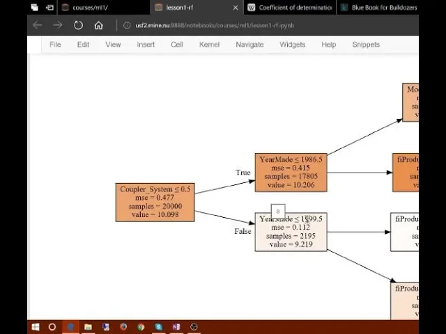
So it first of all decided to split on coupler system greater than or less than 0.5. That's a Boolean variable, so it's actually true or false. And then within the group where a coupler system was true, it decided to split into yearmade greater than or less than 0.987. And then where a coupler system was true and yearmade was less than or equal to 0.986, it used fi_product_class_desk is less than or equal to 0.75, and so forth.

So right at the top, we have 20,000 samples, 20,000 rows. And the reason for that is because that's what we asked for here when we split our data in the sample. I just want to double check that for your decision tree that you have there, that the coloration was whether it's true or false, so it gets darker, it's true for the next one, not the...

Darker is a higher value, we'll get to that in a moment. So let's look at these numbers here. So in the whole data set, our sample that we're using, there are 20,000 rows. The average of the log of price is 10.1. And if we built a model where we just used that average all the time, then the mean squared error would be 0.477.

So this is, in other words, the denominator of an R^2. This is like the most basic model is a tree with zero splits, which is just predict the average. So the best single binary split we can make turns out to be splitting by whether the coupler system is less than or equal to or greater than 0.5, in other words whether it's true or false.

And it turns out if we do that, the mean squared error of coupler system is less than 0.5, so it's false, goes down from 0.477 to 0.11. So it's really improved the error a lot. In the other group, it's only improved it a bit, it's gone from 0.47 to 0.41.

And so we can see that the coupler system equals false group has a pretty small percentage, it's only got 2200 of the 20,000, whereas this other group has a much larger percentage, but it hasn't improved it as much. So let's say you wanted to create a tree with just one split.

So you're just trying to find what is the very best single binary decision you can make for your data. How much you'd be able to do that? How could you do it? I'm going to give it to Ford. But you're writing, you don't have a random forest, right? How are you going to write, what's an algorithm, a simple algorithm which you could use?

Sure. So we want to start building a random forest from scratch. So the first step is to create a tree. The first step to create a tree is to create the first binary decision. How are you going to do it? I'm going to give it to Chris, maybe in two steps.

So isn't this simply trying to find the best predictor based on maybe linear regression? You could use a linear regression, but could you do something much simpler and more complete? We're trying not to use any statistical assumptions here. Can we just take just one variable, if it is true, give it the true thing, and if it is false?

So which variable are we going to choose? So at each binary point we have to choose a variable and something to split on. How are we going to do that? We're going to pass it over there. How do I pronounce your name? Shikhar. So the variable to choose could be like which divides the population into two groups, which are kind of heterogeneous to each other and homogeneous within themselves, like having the same quality within themselves, and they're very different.

Could you be more specific? In terms of the target variable maybe, let's say we have two groups after split, so one has a different price altogether from the second group, but internally they have similar prices. Okay, that's good. So to simplify things a little bit, we're saying find a variable that we could split into such that the two groups are as different to each other as possible.

And how would you pick which variable and which split point? That's the question. What's your first cut? Which variable and which split point? We're making a tree from scratch, we want to create our own tree. Does that make sense? We've got somebody over here, Maisley? Can we test all of the possible splits and see which one has the smallest RMSE?

That sounds good. Okay, so let's dig into this. So when you say test all of the possible splits, what does that mean? How do we enumerate all of the possible splits? For each variable, you could put one aside and then put a second aside and compare the two and if it was better.

Okay, so for each variable, for each possible value of that variable, see whether it's better. Now give it back to Maisley because I want to dig into the better. When you said see if the RMSE is better, what does that mean though? Because after a split, you've got two RMSEs, you've got two groups.

So you're just going to fit with that one variable comparing to the other's not. So what I mean here is that before we decided to split on coupler system, we had a remove the mean squared of 0.477, and after we've got two groups, one with a mean squared error of 0.1, another with a mean squared error of 0.4.

So you treat each individual model separately. So for the first split, you're just going to compare between each variable themselves. And then you move on to the next node with the remaining variable. But even the first node, so the model with zero splits has a single root mean squared error.

The model with one split, so the very first thing we tried, we've now got two groups with two mean squared errors. Do you want to give it to Daniel? Do you pick the one that gets them as different as they can be? Well, okay, that would be one idea.

Get the two mean squared errors as different as possible, but why might that not work? What might be a problem with that? Sample size. Go on. Because you could just literally leave one point out. Yeah, so we could have like year made is less than 1950, and it might have a single sample with a low price, and that's not a great split, is it?

Because the other group is actually not going to be very interesting at all. Can you improve it a bit? Can Jason improve it a bit? Could you take a weighted average? Yeah, a weighted average. So we could take 0.41 times 17,000 plus 0.1 times 2,000. That's good, right? And that would be the same as actually saying I've got a model, the model is a single binary decision, and I'm going to say for everybody with year made less than 986.5, I'm going to fill in 10.2.

For everybody else, I'm going to fill in 9.2, and then I'm going to calculate the root mean squared error of this crappy model. And that will give exactly the same as the weighted average that you're suggesting. So we now have a single number that represents how good a split is, which is the weighted average of the mean squared errors of the two groups it creates.

And thanks to Jake, we have a way to find the best split, which is to try every variable and to try every possible value of that variable and see which variable and which value gives us the split with the best score. That make sense? What's your name? Sorry? Can somebody give Natalie the box?

When you say every possible number for every possible variable, are you saying here we have 0.5 as our criteria to split the tree, are you saying we're trying out every single number for? Every possible value. So a couple of system only has two values, true and false. So there's only one way of splitting, which is trues and falses.

Year made is an integer which varies between 1960 and 2010, so we can just say what are all the possible unique values of year made, and try them all. So we're trying all the possible split points. Can you pass that back to Daniel, or pass it to me and I'll pass it to Daniel?

So I just want to clarify again for the first split. Why did we split on coupler system, true or false to start with? Because what we did was we used Jake's technique. We tried every variable, for every variable we tried every possible split. For each one, we noted down, I think it was Jason's idea, which was the weighted average mean squared error of the two groups we created.

We found which one had the best mean squared error and we picked it, and it turned out it was coupler system, true or false. Does that make sense? I guess my question is more like, so coupler system is one of the best indicators, I guess? It's the best. We tried every variable and every possible level.

So each level after that, it gets less and less? Everything else it tried wasn't as good. And then you do that each time you split? Right. So on that, we now take this group here, everybody who's got coupler system equals true, and we do it again. For every possible variable, for every possible level, for people where coupler system equals true, what's the best possible split?

And then are there circumstances when it's not just like binary? You split it into three groups, for example, year made? So I'm going to make a claim, and then I'm going to see if you can justify it. I'm going to claim that it's never necessary to do more than one split at a level.

Because you can just split it again. Because you can just split it again, exactly. So you can get exactly the same result by splitting twice. So that is the entirety of creating a decision tree. You stop either when you hit some limit that was requested, so we had a limit where we said max depth equals 3.

So that's one way to stop, would be you ask to stop at some point, and so we stop. Otherwise you stop when your leaf nodes, these things at the end are called leaf nodes, when your leaf nodes only have one thing in them. That's a decision tree. That is how we grow a decision tree.

And this decision tree is not very good because it's got a validation R squared of 0.4. So we could try to make it better by removing max depth equals 3 and creating a deeper tree. So it's going to go all the way down, it's going to keep splitting these things further until every leaf node only has one thing in it.

And if we do that, the training R squared is, of course, 1, because we can exactly predict every training element because it's in a leaf node all on its own. But the validation R squared is not one. It's actually better than a really shallow tree, but it's not as good as we'd like.

So we want to find some other way of making these trees better. And the way we're going to do it is to create a forest. So what's a forest? To create a forest, we're going to use a statistical technique called bagging. And you can bag any kind of model.

In fact, Michael Jordan, who is one of the speakers at the recent Data Institute conference here at the University of San Francisco, developed a technique called the Bag of Little Bootstraps, in which he shows how to use bagging for absolutely any kind of model to make it more robust and also to give you confidence intervals.

The random forest is simply a way of bagging trees. So what is bagging? Bagging is a really interesting idea, which is what if we created five different models, each of which was only somewhat predictive, but the models weren't at all correlated with each other. They gave predictions that weren't correlated with each other.

That would mean that the five models would have to have found different insights into the relationships in the data. And so if you took the average of those five models, then you're effectively bringing in the insights from each of them. And so this idea of averaging models is a technique for ensembling, which is really important.

Now let's come up with a more specific idea of how to do this ensembling. What if we created a whole lot of these trees, big, deep, massively overfit trees. But each one, let's say we only pick a random one-tenth of the data. So we pick one out of every ten rows at random, build a deep tree, which is perfect on that subset and kind of crappy on the rest.

Let's say we do that 100 times, a different random sample every time. So all of the trees are going to be better than nothing because they do actually have a real random subset of the data and so they found some insight, but they're also overfitting terribly. But they're all using different random samples, so they all overfit in different ways on different things.

So in other words, they all have errors, but the errors are random. What is the average of a bunch of random errors? Zero. So in other words, if we take the average of these trees, each of which have been trained on a different random subset, the errors will average out to zero, and what's left is the true relationship.

And that's the random forest. So there's the technique. We've got a whole bunch of rows of data. We grab a few at random, put them into a smaller data set, and build a tree based on that. And then we put that tree aside and do it again with a different random subset, and do it again with a different random subset.

Do it a whole bunch of times, and then for each one we can then make predictions by running our test data through the tree to get to the leaf node, take the average in that leaf node for all the trees, and average them all together. So to do that, we simply call random forest regressor, and by default it creates 10 what scikit-learn calls estimators.

An estimator is a tree. So this is going to create 10 trees. And so we go ahead and train it. So create our 10 trees, and we're just doing this on our little random subset of 20,000. And so let's take a look at one example. When you pass the box to Devin.

Just to make sure I'm understanding this, you're saying we take 10 kind of crappy models. We average 10 crappy models, and we get a good model. Exactly. Because the crappy models are based on different random subsets, and so their errors are not correlated with each other. If the errors work correlated with each other, this isn't going to work.

So the key insight here is to construct multiple models which are better than nothing, and where the errors are as much as possible, not correlated with each other. So is there like a certain number of trees that we need that in order to be valid? There's always this thing that's valid or invalid.

There's like, has a good validation set, RMSE, or not. And so that's what we're going to look at, is how to make that metric higher. And so this is the first of our hyperparameters, and we're going to learn about how to tune hyperparameters. And the first one is going to be the number of trees, and we're about to look at that now.

Yes, Maisly. The subset that you're selecting, are they exclusive? Can you have overlapping over them? Yes, so I mentioned one approach would be to pick out a 10th at random, but actually what Scikit-learn does by default is for n rows, it picks out n rows with replacement. And that's called bootstrapping.

And if memory serves me correctly, that gets you an average 63.2% of the rows will be represented, and a bunch of them will be represented multiple times. So rather than just picking out like a 10th of the rows at random, instead we're going to pick out of an n row data set, we're going to pick out n rows with replacement, which on average gets about 63, I think 63.2% of the rows will be represented, many of those rows will appear multiple times.

I think there's a question behind you. In essence, what this model is doing is, if I understand correctly, is just picking out the data points that look most similar to the one you're looking at. Yeah, that's a great insight. So what a tree is kind of doing, there would be other ways of assessing similarity.

There are other ways of assessing similarity, but what's interesting about this way is it's doing it in tree space. So we're basically saying, in this case, for this little tree, what are the 593 samples closest to this one, and what's their average closest in tree space. So other ways of doing that would be like, and we'll learn later on in this course about k nearest neighbors, you could use Euclidean distance.

But here's the thing, the whole point of machine learning is to identify which variables actually matter the most, and how do they relate to each other and your dependent variable together. So imagine a synthetic dataset where you create 5 variables that add together to create your dependent variable, and 95 variables which are entirely random and don't impact your dependent variable.

And then if you do like a k nearest neighbors in Euclidean space, you're going to get meaningless nearest neighbors because most of your columns are actually meaningless. Or imagine your actual relationship is that your dependent variable equals x_1 times x_2. And you'll actually need to find this interaction. So you don't actually care about how close it is to x_1 and how close to x_2, but how close to the product.

So the entire purpose of modeling in machine learning is to find a model which tells you which variables are important and how do they interact together to drive your dependent variable. And so you'll find in practice the difference between using tree space, or random forest space to find your nearest neighbors, versus Euclidean space is the difference between a model that makes good predictions and a model that makes meaningless predictions.

In general, a machine learning model which is effective is one which is accurate when you look at the training data, it's accurate at actually finding the relationships in that training data, and then it generalizes well to new data. And so in bagging, that means that each of your individual estimators, each of your individual trees, you want to be as predictive as possible, but the predictions of your individual trees to be as uncorrelated as possible.

And so the inventor of random forests talks about this at length in his original paper that introduced this in the late 90s, this idea of trying to come up with predictive but poorly correlated trees. The research community in recent years has generally found that the more important thing seems to be creating uncorrelated trees rather than more accurate trees.

So more recent advances tend to create trees which are less predictive on their own, but also less correlated with each other. So for example, in scikit-learn there's another class you can use called extra-trees-aggressor, or extra-trees-classifier with exactly the same API, you can try it tonight, just replace my random forest-aggressor with that, that's called an extremely randomized trees model.

And what that does is exactly the same as what we just discussed, but rather than trying every split of every variable, it randomly tries a few splits of a few variables. So it's much faster to train, it has more randomness, but then with that time you can build more trees and therefore get better generalization.

So in practice, if you've got crappy individual models you just need more trees to get a good end-up model. Okay, so could you pass that over to Devin? Could you talk a little bit more about what you mean by uncorrelated trees? If I build a thousand trees, each one on just 10 data points, then it's quite likely that the 10 data points for every tree are going to be totally different, and so it's quite likely that those 1000 trees are going to give totally different answers to each other.

So the correlation between the predictions of tree 1 and tree 2 is going to be very small, between tree 1 and tree 3 very small, and so forth. On the other hand, if I create a thousand trees where each time I use the entire data set with just one element removed, all those trees are going to be nearly identical, i.e.

their predictions will be highly correlated. And so in the latter case, it's probably not going to generalize very well. Whereas in the former case, the individual trees are not going to be very predictive. So I need to find some nice in-between. I'm just trying to understand how this random forest actually makes sense for continuous variables.

I mean, I'm assuming that you build a tree structure, and the last final nodes you'd be saying like maybe this node represents maybe a category A or a category B, but how does it make sense for a continuous target? So this is actually what we have here, and so the value here is the average.

So this is the average log of price for this subgroup, and that's all we do. The prediction is the average of the value of the dependent variable in that leaf node. So a couple of things to remember, the first is that by default, we're actually going to train the tree all the way down until the leaf nodes are size 1, which means for a data set with n rows, we're going to have n leaf nodes.

And then we're going to have multiple trees, which we averaged together. So in practice, we're going to have lots of different possible values. There's a question behind you? So for the continuous variable, how do we decide which value to split out because there can be many values? We try every possible value of that in the training set.

Won't it be computationally? Computationally expensive. This is where it's very good to remember that your CPU's performance is measured in gigahertz, which is billions of clock cycles per second, and it has multiple cores. And each core has something called SIMD, single instruction multiple data, where it can direct up to 8 computations per core at once.

And then if you do it on the GPU, the performance is measured in teraflops, so trillions of floating point operations per second. And so this is where when it comes to designing algorithms, it's very difficult for us mere humans to realize how stupid algorithms should be, given how fast today's computers are.

So yeah, it's quite a few operations, but at trillions per second, you hardly notice it. Marcia? I have a question. So essentially, at each mode, we make a decision like which category, which variable to use. And which checkpoint? Yes. Yeah, but one thing I can't understand. So we have MSE calculated for each node, right?

So this is kind of one of the decision criteria. But this MSE, it is calculated for which model? Like which model underlies the field? The model is, for the initial root mode, is what if we just predicted the average, right? Which here is 10.098, and just the average. And then the next model is what if we predicted the average of those people with Kepler system equals false, and for those people with Kepler system equals true.

And then the next is, what if we predicted the average of Kepler system equals true, EMA less than 1986? Is it always average, or we can use median, or we can even run linear regression? There's all kinds of things we could do. In practice, the average works really well.

There are types of, they're not called random forests, but there are kinds of trees where the leaf nodes are independent linear regressions. They're not terribly widely used, but there are certainly researchers who have worked on them. Pass it back over there to Ford, and then to Jacob. So this tree has a depth of 3, and then on one of the next commands we get rid of the max depth.

The tree without the max depth, does that contain the tree with the depth of 3? Yeah, except in this case we've added randomness, but if you turn bootstrapping off, the deeper tree will, the less deep tree would be how it would start, and then it just keeps spinning. So you have many trees, you're going to have different leaf nodes across trees, hopefully that's what we want.

So how do you average leaf nodes across different trees? So we just take the first row in the validation set, we run it through the first tree, we find its average, 9.28. Then do it through the next tree, find its average in the second tree, 9.95, and so forth.

And we're about to do that, so you'll see it. So let's try it. So after you've built a random forest, each tree is stored in this attribute called estimators_. So one of the things that you guys need to be very comfortable with is using list comprehensions, so I hope you've all been practicing.

So here I'm using a list comprehension to go through each tree in my model, I'm going to call predict on it with my validation set, and so that's going to give me a list of arrays of predictions. So each array will be all of the predictions for that tree, and I have 10 trees.

np.stack concatenates them together on a new axis. So after I run this and call .shape, you can see I now have the first axis 10, which means I have my 10 different sets of predictions, and for each one my validation set is a size of 12,000, so here are my 12,000 predictions for each of the 10 trees.

So let's take the first row of that and print it out, and so here are 10 predictions, one from each tree. And so then if we say take the mean of that, here is the mean of those 10 predictions, and then what was the actual? The actual was 9.1, our prediction was 9.07.

So you see how none of our individual trees had very good predictions, but the mean of them was actually pretty good. And so when I talk about experimenting, like Jupyter Notebook is great for experimenting, this is the kind of stuff I mean. Dig inside these objects and look at them, plot them, take your own averages, cross-check to make sure that they work the way you thought they did, write your own implementation of R^2, make sure it's the same as a scikit-learn version, plot it.

Here's an interesting plot I did. Let's go through each of the 10 trees and then take the mean of all of the predictions up to the i-th tree. So let's start by predicting just based on the first tree, then the first 2 trees, then the first 3 trees, and let's then plot the R^2.

So here's the R^2 of just the first tree. It's the R^2 of the first 2 trees, 3 trees, 4 trees, up to 10 trees. And so not surprisingly R^2 keeps improving because the more estimators we have, the more bagging that we're doing, the more it's going to generalize. And you should find that that number there, a bit under 0.86, should match this number here.

So again, these are all the cross checks you can do, the things you can visualize to deepen your understanding. So as we add more trees, our R^2 improves, it seems to flatten out after a while. So we might guess that if we increase the number of estimators to 20, it's maybe not going to be that much better.

So let's see, we've got 0.862 versus 0.860, so doubling the number of trees didn't help very much. But double it again, 0.867, double it again, 0.869. So you can see there's some point at which you're going to not want to add more trees, not because it's never going to get worse, because every tree is giving you more semi-random models to bag together, but it's going to stop improving things much.

So this is like the first hyperparameter you'd learn to set is number of estimators, and the method for setting is as many as you have time to fit and that actually seem to be helping. Now in practice, we're going to learn to set a few more hyperparameters, adding more trees slows it down.

But with less trees, you can still get the same insights. So I build most of my models in practice with like 20 to 30 trees, and it's only like then at the end of the project, or maybe at the end of the day's work, I'll then try doing like a thousand trees and run it overnight.

Was there a question? Yes, can we pass that to Prince? So each tree might have different estimators, different combinations of estimators. Each tree is an estimator, so this is a synonym. So in scikit-learn, when they say estimator, they mean tree. So I mean features, each tree might have different breakpoints on different columns.

But if at the end we want to look at the important features? We'll get to that. So after we finish with setting hyperparameters, the next stage of the course will be learning about what it tells us about the data. If you need to know it now, for your projects, feel free to look ahead.

There's a lesson to RF interpretation is where we can see it. So that's our first hyperparameter. I want to talk next about out-of-bag score. Sometimes your data set will be kind of small, and you want to pull out a validation set. Because doing so means you now don't have enough data to build a good model.

What do you do? There's a cool trick which is pretty much unique to random forests, and it's this. What we could do is recognize that some of our rows didn't get used. So what we could do would be to pass those rows through the first tree and treat it as a validation set.

And then for the second tree, we could pass through the rows that weren't used for the second tree through it to create a validation set for that. And so effectively, we would have a different validation set for each tree. And so now to calculate our prediction, we would average all of the trees where that row was not used for training.

So for tree number 1, we would have the ones I've marked in blue here, and then maybe for tree number 2, it turned out it was like this one, this one, this one, and this one, and so forth. So as long as you've got enough trees, every row is going to appear in the out-of-bag sample for one of them, at least.

So you'll be averaging hopefully a few trees. So if you've got 100 trees, it's very likely that all of the rows are going to appear many times in these out-of-bag samples. So what you can do is you can create an out-of-bag prediction by averaging all of the trees you didn't use to train each individual row.

And then you can calculate your root mean squared error, R squared, etc. on that. If you pass oobscore = true to scikit-learn, it will do that for you, and it will create an attribute called oobscore_ and so my little printScore function here, if that attribute exists it adds it to the print.

So if you take a look here, oobscore = true, we've now got one extra number, and it's R squared, that is the R squared for the oob sample, it's R squared is very similar, the R squared and the validation set, which is what we hoped for. Is it the case that the prediction for the oobscore must be mathematically lower than the one for our entire forest?

Certainly it's not true that the prediction is lower, it's possible that the accuracy is lower. It's not mathematically necessary that it's true, but it's going to be true on average because each row appears in less trees in the oob samples than it does in the full set of trees.

So as you see here, it's a little less good. So in general, the OOB R squared will slightly underestimate how generalizable the model is. The more trees you add, the less serious that underestimation is. And for me in practice, I find it's totally good enough in practice. So this OOB score is super handy, and one of the things it's super handy for is you're going to see there's quite a few hyperparameters that we're going to set, and we would like to find some automated way to set them.

And one way to do that is to do what's called a grid search. A grid search is where there's a scikit-learn function called grid search, and you pass in the list of all of the hyperparameters that you want to tune, you pass in for each one a list of all of the values of that hyperparameter you want to try, and it runs your model on every possible combination of all of those hyperparameters and tells you which one is the best.

And OOB score is a great choice for getting it to tell you which one is best in terms of OOB score. That's an example of something you can do with OOB which works well. If you think about it, I kind of did something pretty dumb earlier, which is I took a subset of 30,000 rows of the data and it built all my models of that, which means every tree in my random forest is a different subset of that subset of 30,000.

Why do that? Why not pick a totally different subset of 30,000 each time? So in other words, let's leave the entire 300,000 records as is, and if I want to make things faster, pick a different subset of 30,000 each time. So rather than bootstrapping the entire set of rows, let's just randomly sample a subset of the data.

And so we can do that. So let's go back and recall property F without the subset parameter to get all of our data again. So to remind you, that is 400,000 in the whole data frame of which we have 389,000 in our training set. And instead we're going to go set RF_samples 20,000.

Remember that was the site of the 30,000, we used 20,000 of them in our training set. If I do this, then now when I run a random forest, it's not going to bootstrap an entire set of 391,000 rows, it's going to just grab a subset of 20,000 rows. And so now if I run this, it will still run just as quickly as if I had originally done a random sample of 20,000, but now every tree can have access to the whole data set.

So if I do enough estimators, enough trees, eventually it's going to see everything. So in this case, with 10 trees, which is the default, I get an R^2 of 0.86, which is actually about the same as my R^2 with the 20,000 subset. And that's because I haven't used many estimators yet.

But if I increase the number of estimators, it's going to make more of a difference. So if I increase the number of estimators to 40, it's going to take a little bit longer to run, but it's going to be able to see a larger subset of the data set.

And so as you can see, the R^2 has gone up from 0.86 to 0.876. So this is actually a great approach. And for those of you who are doing the groceries competition, that's got something like 120 million rows. There's no way you would want to create a random forest using 128 million rows in every tree.

It's going to take forever. So what you could do is use this set of samples to do 100,000 or a million. We'll play around with it. So the trick here is that with a random forest using this technique, no data set is too big. I don't care if it's got 100 billion rows.

You can create a bunch of trees, each one of the different random subsets. Can somebody pass the-- actually, I can pass it. So my question was, for the OLB scores and these ones, does it take only for the ones from the sample, or does it take from all the-- That's a great question.

So unfortunately, scikit-learn does not support this functionality out of the box, so I had to write this. And it's kind of a horrible hack, because we'd much rather be passing in like a sample-sized parameter rather than doing this kind of setting up here. So what I actually do is, if you look at the source code, is I'm actually-- this is the internal function I looked at the source code that they call, and I've replaced it with a lambda function that has the behavior we want.

Unfortunately, the current version is not changing how OOB is calculated. So currently, OOB scores and setRF samples are not compatible with each other, so you need to turn OOB equals false if you use this approach. Which I hope to fix, but at this stage it's not fixed. So if you want to turn it off, you just call resetRFSamples, and that returns it back to what it was.

So in practice, when I'm doing interactive machine learning using random forests in order to explore my model, explore hyperparameters, the stuff we're going to learn in the future lesson where we actually analyze feature importance and partial dependence and so forth, I generally use subsets and reasonably small forests because all the insights that I'm going to get are exactly the same as the big ones, but I can run it in like 3 or 4 seconds rather than hours.

So this is one of the biggest tips I can give you, and very few people in industry or academia actually do this. Most people run all of their models on all of the data all of the time using their best possible parameters, which is just pointless. If you're trying to find out which features are important and how are they related to each other and so forth, having that fourth decimal place of accuracy isn't going to change any of your insights at all.

So I would say do most of your models on a large enough sample size that your accuracy is reasonable, when I say reasonable it's like within a reasonable distance of the best accuracy you can get, and it's taking a small number of seconds to train so that you can interactively do your analysis.

So there's a couple more parameters I wanted to talk about, so I'm going to call reset_rf_samples to get back to our full data set, because in this case, at least on this computer, it's actually running in less than 10 seconds. So here's our baseline, we're going to do a baseline with 40 estimators, and so each of those 40 estimators is going to train all the way down until the leaf nodes just have one sample in them.

So that's going to take a few seconds to run, here we go. So that gets us a 0.898r^2 on the validation set, or 0.908 on the OOB. In this case, the OOB is better. Why is it better? Well that's because remember our validation set is not a random sample, our validation set is a different time period, so it's actually much harder to predict a different time period than this one, which is just predicting random.

So that's why this is not the way around we expected. The first parameter we can try fiddling with is min_samples_leaf, and so min_samples_leaf says stop training the tree further when your leaf node has three or less samples in. So rather than going all the way down until there's one, we're going to go down until there's three.

So in practice, this means there's going to be like one or two less levels of decision being made, which means we've got like half the number of actual decision criteria we have to do, so it's going to train more quickly. It means that when we look at an individual tree, rather than just taking one point, we're taking the average of at least three points, that's where we'd expect the trees to generalize each one a little bit better, but each tree is probably going to be slightly less powerful on its own.

So let's try training that. Possible values of min_samples_leaf, I find ones which work well are 1, 3, 5, 10, 25. I find that kind of range seems to work well, but sometimes if you've got a really big data set and you're not using the small samples, you might need a min_samples_leaf of hundreds or thousands.

So you've kind of got to think about how big are your subsamples going through and try things out. In this case, going from the default of 1 to 3 has increased our validations at R squared from 898 to 902, so it's a slight improvement. And it's going to train a little faster as well.

Something else you can try, and since this worked, I'm going to leave that in, I'm going to add in max_features = 0.5. What does max_features do? The idea is that the less correlated your trees are with each other, the better. Now imagine you had one column that was so much better than all of the other columns of being predictive that every single tree you built, regardless of which subset of rows, always started with that column.

So the trees are all going to be pretty similar, but you can imagine there might be some interaction of variables where that interaction is more important than that individual column. So if every tree always fits on the first thing, the same thing the first time, you're not going to get much variation in those trees.

So what we do is, in addition to just taking a subset of rows, we then at every single split point take a different subset of columns. So it's slightly different to the row sampling. For the row sampling, each new tree is based on a random set of rows. For column sampling, every individual binary split we choose from a different subset of columns.

So in other words, rather than looking at every possible level of every possible column, we look at every possible level of a random subset of columns. And each time, each decision point, each binary split, we use a different random subset. How many? Well, you get to pick. Point 5 means randomly choose half of them.

The default is to use all of them. There's also a couple of special values you can use here. As you can see in max_features, you can also pass in square root to get square root of features, or log_2 to get log_2 of features. So in practice, good values I found are range from 1, 0.5, log_2, or square root.

That's going to give you a nice bit of variation. Can somebody pass it to Daniel? So just to clarify, does that just break it up smaller each time it goes through the tree, or is it just taking half of what's left over and hasn't been touched each time? There's no such thing as what's left over.

After you've split on year made less than or greater than 1984, year made is still there. So later on you might then split on year made less than or greater than 1989. So it's just each time, rather than checking every variable to see where it's best split is, you just check half of them.

And so the next time you check a different half. But I mean like in terms as you get further to the leafs, you're going to have less options, right? No, you're not. You never remove the variables. You can use them again and again and again because you've got lots of different split points.

So imagine for example that the relationship was just entirely linear between year made and price. Then in practice to actually model that, your real relationship is year made versus price. But the best we could do would be to first of all split here, and then to split here and here, right?

And like split and split and split. So even if they're binary, most random forest libraries don't do anything special about that. They just kind of go try this variable, oh it turns out there's only one level left. So yeah, definitely they don't do any clever bookkeeping. So if we add max_features=0.5, it goes up from 9.01 to 9.06.

So that's better still. And so as we've been doing this, you've also hopefully noticed that our root mean squared error of log_price has been dropping on our validation set as well. And so it's now down to 0.2286. So how good is that? So like our totally untuned random forest got us in about the top 25%.

Now remember, our validation set isn't identical to the Kaggle test set, and this competition unfortunately is old enough that you can't even put in a kind of after-the-time entry to find out how you would have gone. So we can only approximate how we could have gone, but generally speaking it's going to be a pretty good approximation.

So 2286, here is the competition, here's the public leaderboard, 2286, 14th or 15th place. So roughly speaking, it looks like we would be about in the top 20 of this competition with basically a totally brainless random forest with some totally brainless minor hyperparameter tuning. This is kind of why the random forest is such an important, not just first step, but often only step in machine learning.

Because it's kind of hard to screw it up, even when we didn't tune the hyperparameters, we still got a good result. And then a small amount of hyperparameter tuning got us a much better result. And so any kind of model, and I'm particularly thinking of linear type models, which have a whole bunch of statistical assumptions and you have to get a whole bunch of things right before they start to work at all, can really throw you off track because they give you totally wrong answers about how accurate the predictions can be.

But also the random forest, generally speaking, they tend to work on most data sets most of the time with most sets of hyperparameters. So for example, we did this thing with our categorical variables. In fact let's take a look at our tree. Look at this, f_i_product_class_desk < 7.5. What does that mean?

So f_i_product_class_desk, here are some examples of that column. So what does it mean to be less than or equal to 7? Well we'd have to look at .cat.categories to find out. And so it's 0, 1, 2, 3, 4, 5, 6, 7. So what it's done is it's created a split where all of the backhoe loaders and these three types of hydraulic excavator enter in one group and everything else is in the other group.

So that's weird, like these aren't even in order. We could have made them in order if we had bothered to say the categories have this order, but we hadn't. So how come this even works? Because when we turn it into codes, this is actually what the random forest sees.

And so imagine, to think about this, the only thing that mattered was whether it was a hydraulic excavator of 0-2 metric tons and nothing else mattered, so it has to pick out this single level. Well it can do that because first of all it could say, okay let's pick out everything less than 7 versus greater than 7 to create this as one group and this as another group.

And then within this group, it could then pick out everything less than 6 versus greater than 6, which is going to pick out this one item. So with two split points, we can pull out a single category. So this is why it works, because the tree is infinitely flexible, even with a categorical variable, if there's particular categories which have different levels of price, it can gradually zoom in on those groups by using multiple splits.

Now you can help it by telling it the order of your categorical variable, but even if you don't, it's okay, it's just going to take a few more decisions to get there. And so you can see here it's actually using this product class desk quite a few times. And as you go deeper down the tree, you'll see it used more and more.

Whereas in a linear model, or almost any kind of other model, certainly any non-tree model pretty much, encoding a categorical variable like this won't work at all because there's no linear relationship between totally arbitrary identifiers and anything. So these are the kinds of things that make random forests very easy to use and very resilient.

And so by using that, we've gotten ourselves a model which is clearly world-class at this point already. It's probably well in the top 20 of this Kaggle competition. And then in our next lesson, we're going to learn about how to analyze that model to learn more about the data to make it even better.

So this week, try and really experiment. Have a look inside, try and draw the trees, try and plot the different errors, try maybe using different data sets to see how they work, really experiment to try and get a sense and maybe try to replicate things like write your own R^2, write your own versions of some of these functions, see how much you can really learn about your data set about the random forest.

Great, see you on Thursday. Bye.