OK, hi everybody and welcome to practical deep learning for coders lesson 5. We're at a stage now where we're going to be getting deeper and deeper into the details of how these. Networks actually work last week we saw how to use a slightly lower level library than fast AI being hugging first transformers to train a pretty.

Nice NLP model and today we're going to be. Going back to tabular data and we're going to be trying to build a tabular model actually from scratch. We're going to be able to couple of different types of tabular model from scratch. So the problem that I'm going to be working through is the Titanic problem, which if you remember back a couple of weeks is the data set that we looked at on Microsoft Excel and it has each row is one passenger on the Titanic.

So this is a real world data set. Historic data set tells you both of that passengers survived. What class they were on in the ship, their sex, age, how many siblings, how many other family members, how much they spent in the fair, and whereabouts they embarked one of three different cities.

And you might remember that we built a linear model. We then did the same thing using matrix multiplication, and we also created a very very simple neural network. Um. You know, Excel can do. Nearly everything we need as you saw to build a neural network, but it starts to get unwieldy and so that's why.

People don't use Excel for neural networks in practice. Instead, we use the programming language like Python. So what we're going to do today is we're going to do the same thing. With Python. So we're going to start working through the linear model and neural net from scratch notebook. Which you can find on Kaggle.

Or on the course repository. And today what we're going to do is we're going to work through the one in the clean folder, so both for fast book the book. And course 22 these lessons the clean folder. Contains all of our notebooks, but without. Any pros or any outputs, so here's what it looks like when I open up the linear model and neural net from scratch.

In Jupiter. What I'm using here is. Paper space gradient, just I mentioned a couple of weeks ago, is what I'm going to be doing most things in. It looks a little bit different to the normal paper space gradient. Because the the default view for paper space gradient. At least as I do this course is there rather awkward.

Notebook editor. Which at first glance has the same features as the the real Jupiter notebooks and Jupiter lab environments. But in practice are actually missing lots of things, so this is the. The normal paper space. So remember you have to click this button. Right and the only reason you might keep this window running is then you might go over here to the machine to remind yourself when you close the other tab to click stop machine.

If you're using the free one, it doesn't matter too much. And also when I started, I make sure I've got something to set to shut down automatically. If case I forget. So other than that, we're going to. We can stay in this tab and because Jupiter, this is Jupiter lab that that that runs and you can always switch over.

To classic Jupiter. Notebook if you want to. So given that they're kind of got tabs inside tabs, I normally maximize it at this point. And it's really good at it. Really helpful to know the keyboard shortcuts so control shift square bracket, right and left switch between tabs. That's one of the key things to know about.

OK. So I've opened up the clean version of the. Linear model and neural net from scratch notebook. And so remember when you. Go back through the video kind of the second time or through the notebook a second time. This is generally what you want to be doing is going through the clean notebook and before you run each cell try to think about like, oh, what Jeremy say?

Why are we doing this? What output would I expect? Make sure you get the output you'd expect and if you're not sure why something is the way it is. Try changing it and see what happens and then if you're still not sure why did that thing not work the way I expect.

Search the forum. See if anybody's asked that question before and you can ask the question on the forum yourself if you're still not sure. Um. So as I think we've mentioned briefly before. I find it really nice to be able to use the same notebook both on Kaggle and off Kaggle.

So most of my notebooks start with basically the same cell, which is something that just checks whether we're on Kaggle. So Kaggle sets an environment variable. So we can just check for it in that way. We know if we're on Kaggle. And so then if we are on Kaggle.

You know a notebook that's part of a competition will already have the data downloaded and unzipped for you. Otherwise. If I haven't downloaded the data before, then I need to download it and unzip it OK so. Kaggle is a pip installable module, so you would type pip install Kaggle.

Um. If you're not sure how to do that, you should check our. Deep dive lessons to see exactly the steps, but roughly speaking. You can use your console. Pip install and whatever you want to install. Or as we've seen before, you can do it directly in a notebook. By putting an explanation mark at the start.

So that's going to run not Python, but a shell command. OK, so that's enough to ensure that we have the data downloaded and a variable called path that's pointing at it. Um, most of the time we're going to be using at least PyTorch and NumPy, so we import those so that they're available to Python, and when we're working with tabular data, as we talked about before.

We're generally also going to want to use pandas, and it's really important that you're somewhat familiar with the kind of basic API of these. Three libraries and I've recommended Wes McKinney's book before, particularly for these ones. Um, one thing just by the way is that these things tend to assume you've got a very narrow screen, which is really annoying 'cause it always wraps things.

So if you want to put these three lines as well, then it just makes sure that everything is going to use up the screen properly. OK, so as we've seen before, you can read a common separated values file with pandas. And you can take a look at the first few lines and last few lines and how big it is.

And so here's the same thing as our spreadsheet. OK, so there's our data from the spreadsheet, and here it is as a data frame. So. If we go. Data frame dot is. NA. That returns a new data frame in which every column it tells us whether or not. That particular value is.

Nan so Nan is not a number and most written norm. The most common reason you get that is because it was missing. OK, so a missing value is obviously not a number. So we in the Excel version we did something you should never usually do. We deleted all the rows with missing data.

Just because in Excel it's a little bit harder to work with in pandas, it's very easy to work with. First of all. We can just sum up what I just showed you. Now if you call some on a data frame, it sums up each column, right? So you can see that there's kind of some.

Small foundational concepts in pandas, which when you put them together, take you a long way. So one idea is this idea that you can park. You can call a method on a data frame and it calls it on every row. And then you can call a reduction on that and it reduces.

Each column and so now we've got the total and. In Python and pandas and NumPy and PyTorch, you can treat a Boolean as a number and true will be one. False will be zero. So this is the number of missing values in each column. So we can see that cabin at 891 rows.

It's nearly always empty. Age is empty a bit of the time, but it's almost never empty. So. If you remember from Excel. We need to multiply a coefficient. By each column, that's how we create a linear model. So how would you multiply a coefficient by a missing value? You can't.

There's lots of ways of it's called imputing missing values, so replacing missing value with a number. There is yes, which always works is to replace missing values with the mode of a column. The mode is the most common value that works both the categorical variables is the most common category and continuous variables.

That's the most common. Number so you can get the mode. By calling. DF dot mode, one thing that's a bit awkward is that if there's a tie for the mode, so there's more than one thing that's that's the most common, it's going to return multiple rows, so I need to return the zeroth row.

So here is the mode of every column, so we can replace the missing values for age with 24 and the missing values for cabin with. B96 be 98 and embarked with S. Um, I'll just mention in passing. I am not going to describe every single method we call in every single function we use.

And that is not because. You're an idiot if you don't already know them. Nobody knows them all right, but I don't know which particular subset of them you don't know right? So let's assume just to pick a number at random that the average fast AI student knows 80% of the functions we call.

And then. I could tell you. What every function is, in which case 80% of the time I'm wasting your time to already know. Um, or I could pick 20% of them at random, in which case I'm still not helping 'cause most of the time it's not the ones you don't know.

My approach is that for the ones that are pretty common, I'm just not going to mention it at all because I'm assuming that you'll Google it right. So it's really important to know. So for example, if you don't know what I lock is. That's not a problem. It doesn't mean you're stupid, right?

It just means you haven't used it yet. And you should Google it, right? So I mentioned in this particular case, you know, this is one of the most important pandas, methods because it gives you the row located at this index. I for index and lock for location. So this is a zero through.

But yeah, I did kind of go through things a little bit quickly. On the assumption that students fast AI students are, you know, proactive curious people. And if you're not a proactive curious person, then you could either decide to become one for the purpose of this course or maybe this course isn't for you.

Alright, so a data frame. Has a very convenient method called fill NA and that's going to replace the not a numbers with whatever I put here. And the nice thing about pandas is it kind of has this understanding that columns match to columns, it's going to take the the mode from each column.

And match it to the same column in the data frame and fill in those missing values. Normally that would return a new data frame. Many things, including this one in pandas, have an in place argument that says actually modify the original one. And so if I run that. Now if I call .isna.sum.

They're all zero, so that's like the world's simplest way. To get rid of missing values, OK, so. Why did we do it the world's simplest way? Because honestly. This doesn't make much difference most of the time, and so I'm not going to spend time the first time I go through and build a baseline model.

Doing complicated things when I don't necessarily know that we need complicated things. And so imputing missing values is an example of something that most of the time this dumb way, which always works without even thinking about it, will be quite good enough, you know, for nearly all the time.

So we keep things simple where we can. John, question. Jeremy, we've got a question on this topic. Javier is sort of commenting on the assumption involved in substituting with the mode and he's asking in your experience, what are the pros and cons of doing this versus, for example, discarding cabin or age as fields that we even train the model?

Yeah, so I would certainly never throw him out, right? That there's just no reason to throw away data, and there's lots of reasons to not throw away data. So for example. When we use the fast AI library, which we'll use later, one of the things it does, which is actually a really good idea, is it creates a new column.

For everything that's got missing values, which is Boolean, which is did that column have a missing value for this row? And so maybe it turns out that. Cabin being empty is a great predictor. So yeah, I don't throw out rows and I don't throw out columns. OK, so. It's helpful to understand a bit more about our data set and a really helpful.

I've already imported this. A really helpful, you know, quick method and again, it's kind of nice to know like a few. Quick things you can do to get a picture of what's happening in your data is described. And so describe you can say OK, describe all the numeric variables.

And that gives me a quick sense. Of what's going on here so we can see survived clearly is just zeros and ones. 'cause all of the quartiles are zeros and ones. Looks like P class is 123. What else do we see fairs and interesting one, right? Lots of smallish numbers and one really big numbers are probably long tailed.

So yeah, good to have a look at this to see what's what's going on for your numeric variables. So as I said, fair looks kind of interesting. To find out what's going on there, I would generally go with a histogram. So if you can't quite remember histogram is again, Google it, but in short it shows you for each amount of fair.

How often does that fair appear? And it shows me here that the vast majority of fairs are less than $50, but there's a few right up here to 500. So this is what we call a long tailed distribution. A small number of really big. Values and lots of small ones.

There are some types of model which do not like long tail distributions. Linear models are certainly one of them and neural nets are generally better behaved without them as well. Luckily there's a almost surefire way to turn a long tail distribution into a more reasonably centered distribution, and that is to take the log.

We use logs a lot in machine learning. For those of you that haven't touched them since year 10 math. It would be a very good time to like go to Khan Academy or something and remind yourself about what logs are and what they look like, 'cause they're actually really, really important.

But the basic shape of the log curve causes it to make you know really big numbers less really big and doesn't change really small numbers very much at all. So if we take the log now log of 0 is nan. So a useful trick is to just do log plus one.

And in fact, there is a log P1 if you want to do that does the same thing. So if we look at the histogram of that, you can see it's much more. You know. Sensible now it's kind of centered and it doesn't have this big long tail, so that's pretty good so.

We'll be using that column in the future. As a rule of thumb. Stuff like money or population things that kind of can grow exponentially, you very often want to take the log of. So if you have a column with $1 sign on it, that's a good sign. It might be something to take the log of.

So there was another one here, which is we had a numeric. Which actually doesn't look numeric at all. It looks like it's actually categories. So pandas gives us a dot unique. And so we can see, yeah, they're just one, two and three or the levels of. P class that's their first class, second class or third class.

We can also describe all the non numeric variables. And so we can see here that not surprisingly names are unique 'cause the count of names is the same as count unique is two sexes. 681 different tickets. 147 different cabins and three levels of embarked. So. We cannot multiply the letter S.

By a coefficient. Or the word male. By a coefficient. So what do we do? What we do is we create something called dummy variables. Dummy variables are. And we can just go get dummies. A column that says, for example, is sex female, is sex male, is P class one, is P class two, is P class three.

So for every possible level of every possible categorical variable, it's a Boolean column of did that row have that value of that column? So I think we've briefly talked about this before, that there's a couple of different ways we can do this. One is that for an N level categorical variable, we could use N minus one levels.

In which case we also need a constant term in our model. Pandas by default shows all N levels, although you can pass an argument to change that if you want. Yeah, drop first. I kind of like having all of them sometimes 'cause then you don't have to put in a constant term and it's a bit less annoying and it can be a bit easier to interpret, but I don't feel strongly about it either way.

Okay, so here's a list of all of the columns that pandas added. I guess strictly speaking, I probably should have automated that, but nevermind. I just copied and pasted them. And so here are a few examples of the added columns. In Unix, pandas, lots of things like that. Head means the first few rows or the first few lines.

So five by default and pandas. So here you can see they're never both male and female. They're never neither. They're always one or the other. All right, so with that now we've got numbers which we can multiply by coefficients. It's not gonna work for name, obviously, 'cause we'd have 891 columns and all of them would be unique.

So we'll ignore that for now. That doesn't mean it's have to always ignore it. And in fact, something I did do, something I did do on the forum topic 'cause I made a list of some nice Titanic notebooks that I found. And quite a few of them really go hard on this name column.

And in fact, one of them, yeah, this one, in what I believe is, yes, Christiot's first ever Kaggle notebook. He's now the number one ranked Kaggle notebook person in the world. So this is a very good start. He got a much better score than any model that we're gonna create in this course using only that column name.

And basically, yeah, he came up with this simple little decision tree by recognizing all of the information that's in a name column. So yeah, we don't have to treat a big string of letters like this as a random big string of letters. We can use our domain expertise to recognize that things like Mr.

have meaning and that people with the same surname might be in the same family and actually figure out quite a lot from that. But that's not something I'm gonna do. I'll let you look at those notebooks if you're interested in the feature engineering. And I do think that they're very interesting.

So do check them out. Our focus today is on building a linear model and a neural net from scratch, not on tabular feature engineering, even though that's also a very important subject. Okay, so we talked about how matrix multiplication makes linear models much easier. And the other thing we did in Excel was element-wise multiplication.

Both of those things are much easier if we use PyTorch instead of plain Python, or we could use NumPy. But I tend to just stick with PyTorch when I can 'cause it's easier to learn one library than two. So I just do everything in PyTorch. I almost never touch NumPy nowadays.

They're both great, but they do everything each other does except PyTorch also does differentiation and GPUs. So why not just learn PyTorch? So to turn a column into something that I can do PyTorch calculations on, I have to turn it into a tensor. So a tensor is just what NumPy calls an array.

It's what mathematicians will call either a vector or a matrix, or once we go to higher ranks, mathematicians and physicists just call them tensors. In fact, this idea originally in computer science came from a notation developed in the '50s called APL, which was turned into a programming language in the '60s by a guy called Ken Iverson.

And Ken Iverson actually came up with this idea from, he said, his time doing tensor analysis in physics. So these areas are very related. So we can turn the survived column into a tensor and we'll call that tensor our dependent variable. That's the thing we're trying to predict. Okay, so now we need some independent variables.

So our independent variables are age, siblings, that one is, oh yeah, number of other family members, the log affair that we just created plus all of those dummy columns we added. And so we can now grab those values and turn them into a tensor and we have to make sure they're floats.

We want them all to be the same data type and PyTorch wants things to be floats if you're gonna multiply things together. So there we are. And so one of the most important attributes of a tensor, probably the most important attribute is its shape, which is how many rows does it have and how many columns does it have?

The length of the shape is called its rank. That's the rank of the tensor. It's the number of dimensions or axes that it has. So a vector is rank one, a matrix is rank two, a scalar is rank zero and so forth. I try not to use too much jargon, but there's some pieces of jargon that are really important 'cause like otherwise you're gonna have to say the length of the shape again and again.

It's much easier to say rank. So we'll use that word a lot. So a table is a rank two tensor. Okay, so we've now got the data in good shape. Here's our independent variables and we've got our dependent variable. So we can now go ahead and do exactly what we did in Excel, which is to multiply our rows of data by some coefficients.

And remember to start with we create random coefficients. So we're gonna need one coefficient for each column. Now in Excel we also had a constant, but in our case now we've got every column, every level in our dummy variables, so we don't need a constant. So the number of coefficients we need is equal to the shape of the independent variables and it's the index one element.

That's the number of columns. So that's how many coefficients we want. So we can now ask PyTorch to give us some random numbers and cof of them. They're between zero and one. So if we subtract a half then they'll be centered. And there we go. Before I do that, I set the seed.

What that means is in computers, computers in general cannot create truly random numbers. Instead they can calculate a sequence of numbers that behave in a random like way. That's actually good for us because often in my teaching I like to be able to say, you know, in the pros, oh look, that was two, now it's three or whatever.

And if I was using really random numbers, then I couldn't do that because it'd be different each time. So this makes my results reproducible. That means if you run it, you'll get the same random numbers as I do by saying start the pseudo random sequence with this number. I mentioned in passing, a lot of people are very, very into reproducible results.

They think it's really important to always do this. I strongly disagree with that. In my opinion, an important part of understanding your data is understanding how much it varies from run to run. So if I'm not teaching and wanting to be able to write things about these pseudo random numbers, I almost never use a manual seed.

Instead I like to run things a few times and get an intuitive sense of like, oh, this is like very, very stable. Or, oh, this is all over the place. I'm getting an intuitive understanding of how your data behaves and your model behaves is really important. Now here's one of the coolest lines of code you'll ever see.

I know it doesn't look like much, but think about what it's doing. Yeah, that'll do. Okay, so we've multiplied a matrix by a vector. Now that's pretty interesting. Now mathematicians amongst you will know that you can certainly do a matrix vector product, but that's not what we've done here at all.

We've used element-wise multiplication. So normally if we did the element-wise multiplication of two vectors, it would multiply element one with element one, element two with element two, and so forth and create a vector of the same size output. But here we've done a matrix times a vector. How does that work?

This is using the incredibly powerful technique of broadcasting. And broadcasting again comes from APL, a notation invented in the '50s and a programming language developed in the '60s. And it's got a number of benefits. Basically what it's gonna do is it's gonna take each coefficient and multiply them in turn by every row in our matrix.

So if you look at the shape of our independent variable and the shape of our coefficients, you can see that each one of these coefficients can be multiplied by each of these 891 values in turn. And so the reason we call it broadcasting is it's as if this is 891 columns by 12, rows by 12 columns.

It's as if this was broadcast 891 times. It's as if we had a loop, looping 891 times and doing coefficients times row zero, coefficients times row one, coefficients times row zero, two, and so forth, which is exactly what we want. Now, reasons to use broadcasting, obviously the code is much more concise.

It looks more like math rather than clunky programming with lots of boilerplate, so that's good. Also, that broadcasting all happened in optimized C code. And if in fact it's being done on a GPU, it's being done in optimized GPU assembler, CUDA code. It's gonna run very, very fast indeed.

And this is a trick of why we can use a so-called slow language like Python to do very fast big models is because a single line of code like this can run very quickly on optimized hardware on lots and lots of data. The rules of broadcasting are a little bit subtle and important to know.

And so I would strongly encourage you to Google NumPy broadcasting rules and see exactly how they work. But the kind of intuitive understanding of them, hopefully you'll get pretty quickly, which is generally speaking, you can kind of, as long as the last axes match, it'll broadcast over those axes.

You can broadcast a rank three thing with a rank one thing or a simple version would be tensor one, two, three times two. So broadcast a scalar over a vector. That's exactly what you would expect. So it's copying effectively that two into each of these spots, multiplying them together, but it doesn't use it up any memory to do that.

It's kind of a virtual copying if you like. So this line of code independence by coefficients is very, very important. And it's the key step that we wanted to take, which is now we know exactly what happens when we multiply the coefficients in. And if you remember back to Excel, we did that product and then in Excel, there's a sum product, we then added it all together because that's what a linear model is.

It's the coefficients times the values added together. So we're now gonna need to add those together. But before we do that, if we did add up this row, you can see that the very first value has a very large magnitude and all the other ones are small. Same with row two, same with row three, same with row four.

What's going on here? Well, what's going on is that the very first column was age. And age is much bigger than any of the other columns. It's not the end of the world, but it's not ideal, right? Because it means that a coefficient of say 0.5 times age means something very different to a coefficient of say 0.5 times log fair, right?

And that means that that random coefficient we start with, it's gonna mean very different things for very different columns. And that's gonna make it really hard to optimize. So we would like all the columns to have about the same range. So what we could do as we did in Excel is to divide them by the maximum.

So the maximum, so we did it for age and we also did it for fair. In this case, I didn't use log. So we can get the max of each row by calling .max. And you can pass in a dimension. Do you want the maximum of the rows or the maximum of the columns?

We want the maximum over the rows. So we pass in dimension zero. So those different parts of the shape are called either axes or dimensions. PyTorch calls them dimensions. So that's gonna give us the maximum of each row. And if you look at the docs for PyTorch's max function, it'll tell you it returns two things, the actual value of each maximum and the index of which row it was.

We want the values. So now, thanks to broadcasting, we can just say take the independent variables and divide them by the vector of values. Again, we've got a matrix and a vector. And so this is gonna do an element-wise division of each row of this divided by this vector.

Again, in a very optimized way. So if we now look at our normalized independent variables by the coefficients, you can see they're all pretty similar values. So that's good. There's lots of different ways of normalizing, but the main ones you'll come across is either dividing by the maximum or subtracting the mean and dividing by the standard deviation.

It normally doesn't matter too much. 'Cause I'm lazy, I just picked the easier one. And being lazy and picking the easier one is a very good plan in my opinion. So now that we've conceived that multiplying them together is working pretty well, we can now add them up. And now we want to add up over the columns.

And that would give us predictions. Now obviously, just like in Excel, when we started out, they're not useful predictions 'cause they're random coefficients, but they are predictions nonetheless. And here's the first 10 of them. So then remember, we want to use gradient descent to try to make these better.

So to do gradient descent, we need a loss. The loss is the measure of how good or bad are these coefficients. My favorite loss function as a kind of like, don't think about it, just chuck something out there, is the mean absolute value. And here it is, torch.absoluteValue of the error, difference, take the mean.

And often stuff like this, you'll see people will use pre-written mean absolute error functions, which is also fine, but I quite like to write it out 'cause I can see exactly what's going on. No confusion, no chance of misunderstanding. So those are all the steps I'm gonna need to create coefficients, run a linear model, and get its loss.

So what I like to do in my notebooks, like not just for teaching, but all the time, is to like do everything step-by-step manually, and then just copy and paste the steps into a function. So here's my calc_pretz function, is exactly what I just did, right? Here's my calc_loss function, exactly what I just did.

And that way, a lot of people like go back and delete all their explorations, or they like do them in a different notebook, or they're like working in an IDE, they'll go and do it in some line-oriented repo, whatever. But if you think about the benefits of keeping it here, when you come back to it in six months, you'll see exactly why you did what you did and how we got there, or if you're showing it to your boss or your colleague, you can see exactly what's happening, what does each step look like.

I think this is really very helpful indeed. I know not many people code that way, but I feel strongly that it's a huge productivity win to individuals and teams. So remember from our gradient descent from scratch that the one bit we don't wanna do from scratch is calculating derivatives, 'cause it's just menial and boring.

So to get PyTorch to do it for us, you have to say, well, what things do you want derivatives for? And of course, we want it for the coefficients. So then we have to say requires_grad. And remember, very important, in PyTorch, if there's an underscore at the end, that's an in-place operation.

So this is actually gonna change coefficients. It also returns them, right? But it also changes them in place. So now we've got exactly the same numbers as before, but with requires_grad turned on. So now when we calculate our loss, that doesn't do any other calculations, but what it does store is a gradient function.

It's the function that Python has remembered that it would have to do to undo those steps to get back to the gradient. And to say, oh, please actually call that backward gradient function, you call backward. And at that point, it sticks into a .grad attribute, the coefficients gradients. So this tells us that if we increased the age coefficient, the loss would go down.

So therefore we should do that, right? So since negative means increasing this would decrease the loss, that means we need to, if you remember back to the gradient descent from scratch notebook, we need to subtract the coefficients times the learning rate. So we haven't got any particular ideas yet of how to set the learning rate.

So for now, I just pick a, just try a few and still find out what works best. In this case, I found .1 worked pretty well. So I now subtract. So again, this is sub_, so subtract in place from the coefficients, the gradient times the learning rate. And so the loss has gone down.

That's great from .54 to .52. So there is one step. So we've now got everything we need to train a linear model. So let's do it. Now, as we discussed last week, to see whether your model's any good, it's important that you split your data into training and validation.

For the Titanic dataset, it's actually pretty much fine to use a random split because back when my friend Margit and I actually created this competition for Kaggle many years ago, that's basically what we did, if I remember correctly. So we can split them randomly into a training set and a validation set.

So we're just gonna use fast_ai for that. It's very easy to do it manually with NumPy or PyTorch. You can use scikit_learns, train_test_split. I'm using fast_ai's here, partly because it's easy just to remember one way to do things and this works everywhere. And partly because in the next notebook, we're gonna be seeing how to do more stuff in fast_ai.

So I wanna make sure we have exactly the same split. So those are a list of the indexes of the rows that will be, for example, in the validation set. That's why I call it validation split. So to create the validation independent variables, you have to use those to index into the independent variables and ditto for the dependent variables.

And so now we've got our independent variable training set and our validation set, and we've also got the same for the dependent variables. So like I said before, I normally take stuff that I've already done in a notebook, seems to be working and put them into functions. So here's the step which actually updates coefficients.

So let's chuck that into a function. And then the steps that go cat_loss, start_backward, update_coefficients, and then print the loss or chuck that in one function. So just copying and pasting stuff into cells here. And then the bit on the very top of the previous section that got the random numbers, minus 0.5 requires grad, chuck that in the function.

So here we've got something that initializes coefficients, something that does one epoch by updating coefficients. So we can put that together into something that trains the model for any epochs with some learning rate by setting the manual seed, initializing the coefficients, doing one epoch in a loop, and then return the coefficients.

So let's go ahead and run that function. So it's printing at the end of each one the loss, and you can see the loss going down from 0.53, down, down, down, down, down, to a bit under 0.3. So that's good. We have successfully built and trained a linear model on a real dataset.

I mean, it's a Kaggle dataset, but it's important to not underestimate how real Kaggle datasets are, they're real data. And this one's a playground dataset, so it's not like anybody actually cares about predicting who survived the Titanic, 'cause we already know. But it has all the same features of different data types and missing values and normalization and so forth.

So it's a good playground. So it'd be nice to see what the coefficients are attached to each variable. So if we just zip together the independent variables and the coefficients, and we don't need the regret anymore, and create a dict of that, there we go. So it looks like older people had less chance of surviving.

That makes sense. Males had less chance of surviving. Also makes sense. So it's good to kind of eyeball these and check that they seem reasonable. Now the metric for this Kaggle competition is not main absolute error, it's accuracy. Now, of course, we can't use accuracy as a loss function 'cause it doesn't have a sensible gradient, really.

But we should measure accuracy to see how we're doing because that's gonna tell us how we're going against the thing that the Kaggle competition cares about. So we can calculate our predictions. And we'll just say, okay, well, any times the predictions over 0.5, we'll say that's predicting survival. So that's our predictors of survival.

This is the actual in a validation set. So if they're the same, then we predicted it correctly. So here's, are we right or wrong for the first 16 rows? We're right more often than not. So if we take the mean of those, remember true equals one, then that's our accuracy.

So we are right about 79% of the time. That's not bad, okay? So we've successfully created something that's actually predicting who survived the Titanic. That's cool, from scratch. So let's create a function for that, an accuracy function that just does what I showed. And there it is. Now, I'll say another thing like, my weird coding thing for me, weird as in not that common, is I use less comments than most people because all of my code lives in notebooks.

And of course, in the real version of this notebook is full of pros, right? So when I've taken people through a whole journey about what I've built here and why I've built it and what intermediate results are and check them along the way, the function itself, for me, doesn't need extensive comments.

I'd rather explain the thinking of how I got there and show examples of how to use it and so forth. Okay, now, here's the first few predictions we made. And some of the time, we're predicting negatives for survival and greater than one for survival, which doesn't really make much sense, right?

People either survived one or they didn't, zero. It would be nice if we had a way to automatically squish everything between zero and one. That's gonna make it much easier to optimize. The optimizer doesn't have to try hard to hit exactly one or hit exactly zero, but it can just try to create a really big number to mean survive to a really small number to mean perished.

Here's a great function. Here's a function that as I increase, let's make it even bigger, range. As my numbers get beyond four or five, it's asymptoting to one. And on the negative side, as they get beyond negative four or five, they asymptote to zero. Or to zoom in a bit.

But then around about zero, it's pretty much a straight line. This is actually perfect. This is exactly what we want. So here is the equation, one over one plus eight of the negative minus X. And this is called the sigmoid function. By the way, if you haven't checked out SymPy before, definitely do so.

This is the symbolic Python package, which can do, it's kind of like Mathematica or Wolfram style symbolic calculations, including the ability to plot symbolic expressions, which is pretty nice. PyTorch already has a sigmoid function. I mean, it just calculates this, but it does it in an all optimized way.

So what if we replaced calc preds? Remember before calc preds was just this. What if we took that and then put it through a sigmoid? So calc preds were now basically the bigger, oops. The bigger this number is, the closer it's gonna get to one. And the smaller it is, the closer it's gonna get to zero.

There should be a much easier thing to optimize and ensures that all of our values are in a sensible range. Now, here's another cool thing about using Jupyter plus Python. Python is a dynamic language. Even though I called calc preds, train model calls one epoch, which calls calc loss, which calls calc preds.

I can redefine calc preds now, and I don't have to do anything. That's now inserted into Python symbol table, and that's the calc preds that train model will eventually call. So if I now call train model, that's actually gonna call my new version of calc preds. So that's a really neat way of doing exploratory programming in Python.

I wouldn't release a library that redefines calc preds multiple times. When I'm done, I would just keep the final version, of course. But it's a great way to try things, as you'll see. And so look what's happened. I found I was able to increase the learning rate from 0.1 to two.

Yeah, it was much easier to optimise, as I guessed. And the loss has improved from 0.295 to 0.197. The accuracy has improved from 0.79 to 0.82, nearly 0.83. So as a rule, this is something that we're pretty much always gonna do when we have a binary dependent variable. So dependent variable that's one or zero.

Is the very last step is chuck it through a sigmoid. Generally speaking, if you're wondering, why is my model with a binary dependent variable not training very well? This is the thing you wanna check. Oh, are you chucking it through a sigmoid? Or is the thing you're calling chucking it through a sigmoid or not?

It can be surprisingly hard to find out if that's happening. So for example, with hugging face transformers, I actually found I had to look in their source code to find out. And I discovered that something I was doing wasn't and didn't seem to be documented anywhere. But it is important to find these things out.

As we'll discuss in the next lesson, we'll talk a lot about neural net architecture details, but the details we'll focus on what happens to the inputs at the very first stage and what happens to the outputs at the very last stage. We'll talk a bit about what happens in the middle, but a lot less.

And the reason why is it's the things that you put into the inputs that's gonna change for every single data set you do. And what do you wanna happen to the outputs? It's just gonna happen for every different target that you're trying to hit. So those are the things that you actually need to know about.

So for example, this thing of like, well, you need to know about the sigmoid function and you need to know that you need to use it. Fast AI is very good at handling this for you. That's why we haven't had to talk about it much until now. If you say, oh, it's a category block dependent variable, you know, it's gonna use the right kind of thing for you.

But most things are not so convenient. John's question. - Yes, there is. It's back in the sort of the feature engineering topic, but a couple of people have liked it. So I thought we'd put it out there. So Shivam says one concern I have while using get dummies, so it's in that get dummies phase, is what happens while using test data?

I have a new category, let's say male, female and other. And this will have an extra column missing from the training data. How do you take care of that? - That's a great question. Yeah, so, normally you've got to think about this pretty carefully and check pretty carefully, unless you use fast AI.

So fast AI always creates an extra category called other, and at test time, inference time, if you have some level that didn't exist before, we put it into the other category for you. Otherwise, you basically have to do that yourself, or at least check. Generally speaking, it's pretty likely that otherwise, your extra level will be silently ignored, 'cause it's gonna be in the dataset, but it's not gonna be matched to a column.

So yeah, it's a good point, and definitely worth checking. For categorical variables with lots of levels, I actually normally like to put the less common ones into an other category. And again, that's something that fast AI will do for you automatically. But yeah, definitely something to keep an eye out for.

Good question. Okay, so before we take our break, we'll just do one last thing, which is we will submit this to Kaggle, because I think it's quite cool that we have successfully built a model from scratch. So Kaggle provides us with a test.csv, which is exactly the same structure as the training CSV, except that it doesn't have a survived column.

Now interestingly, when I tried to submit to Kaggle, I got an error in my code saying that, oh, one of my fares is empty. So that was interesting, because the training set doesn't have any empty fares. So sometimes this will happen, that the training set and the test set have different things to deal with.

So in this case, I just said, oh, there's only one row, I don't care. So I just replaced the empty one with a zero for fare. So then I just copied and pasted the pre-processing steps from my training data frame, and stuck them here for the test data frame and the normalization as well.

And so now I just call countPrets, is it greater than 0.5? Turn it into a zero or one, because that's what Kaggle expects, and put that into the survived column, which previously, remember, didn't exist. So then finally I created data frame with just the two columns ID and survived.

Stick it in a CSV file, and then I can call the Unix command head, just to look at the first few rows. And if you look at the Kaggle competition's data page, you'll see this is what the submission file is expected to look like, so that made me feel good.

So I went ahead and submitted it. Oh, I didn't mention it. Okay, so anyway, I submitted it, and I remember I got like, I think I was basically right in the middle, about 50%, you know, better than half the people who have entered the competition, worse than half the people.

So, you know, solid middle of the pack result for a linear model from scratch, I think's a pretty good result. So that's a great place to start. So let's take a 10-minute break. We'll come back at 7.17 and continue on our journey. All right, welcome back. You might remember from Excel that after we did the some product version, we then replaced it with a matrix model play.

Wait, not there, must be here. Here we are, with a matrix model play. So let's do that step now. So matrix times vector dot sum over axis equals one is the same thing as matrix model play. So here is the times dot sum version. Now we can't use this character for a matrix model play 'cause it means element wise operation.

All of the times plus minus divide in PyTorch NumPy mean element wise. So corresponding elements. So in Python instead, we use this character. As far as I know, it's pretty arbitrary. It's one of the ones that wasn't used. So that is an official Python, it's a bit unusual. It's an official Python operator, it means matrix model play, but Python doesn't come with an implementation of it.

So because we've imported, because these are tensors and in PyTorch it will use PyTorches. And as you can see, they're exactly the same. So we can now just simplify a little bit what we had before. Calc preds is now torch dot sigmoid of the matrix model play. Now there is one thing I'd like to move towards now is that we're gonna try to create a neural net in a moment.

And so that means rather than treat this as a matrix times a vector, I wanna treat this as a matrix times a matrix because we're about to add some more columns of coefficients. So we're gonna change in a coefs so that rather than creating an n coef vector, we're gonna create an n coef by one matrix.

So in math, we would probably call that a column vector, but I think that's a kind of a dumb name in some ways 'cause it's a matrix, right? It's a rank two tensor. So the matrix model play will work fine either way, but the key difference is that if we do it this way, then the result of the matrix model play will also be a matrix.

It'll be again, a n rows by one matrix. That means when we compare it to the dependent variable, we need the dependent variable to be an n rows by one matrix as well. So effectively, we need to take the n rows long vector and turn it into an n rows by one matrix.

So there's some useful, very useful, and at first maybe a bit weird notation in PyTorch NumPy for this, which is if I take my training dependent variables vector, I index into it and colon means every row, right? So in other words, that just means the whole vector, right? It's the same basically as that.

And then I index into a second dimension. Now this doesn't have a second dimension. So there's a special thing you can do, which is if you index into a second dimension with a special value none, it creates that dimension. So this has the effect of adding an extra trailing dimension to train dependence.

So it turns it from a vector to a matrix with one column. So if we look at the shape after that, as you see, it's now got, we call this a unit axis. It's got a trailing unit axis, 713 rows and one column. So now if we train our model, we'll get coefficients just like before, except that it's now a column vector, also known as a rank two matrix with a trailing unit axis.

Okay, so that hasn't changed anything. It's just repeated what we did in the previous section, but it's kind of set us up to expand because now that we've done this using matrix multiply, we can go crazy and we can go ahead and create a neural network. So with our neural network, remember back to the Excel days, notice here it's the same thing, right?

We created a column vector, but we didn't create a column vector, we actually created a matrix with kind of two sets of coefficients. So when we did our matrix multiply, every row gave us two sets of outputs, which we then chucked through value, right? Which remember we just used an if statement and we added them together.

So our co-effs now to make a proper neural net, we need one set of co-effs here, and so here they are, torch.rand and co-eff by what? Well, in Excel, we just did two because I kind of got bored of getting everything working properly, but you don't have to worry about feeling rash and creating columns and blah, blah, blah, and in PyTorch, you can create as many as you like.

So I made it something you can change, I called it nhidden, number of hidden activations, and I just set it to 20. And as before, we centralized them by making them go from minus 0.5 to 0.5. Now, when you do stuff by hand, everything does get more fiddly. If our coefficients aren't, if they're too big or too small, it's not gonna train at all.

Basically, the gradients will kind of vaguely point in the right direction, but you'll jump too far or not far enough or whatever. So I want my gradients to be about the same as they were before. So I divide by nhidden, because otherwise at the next step, when I add up the next matrix multiply, it's gonna be much bigger than it was before.

So it's all very fiddly. So then I wanna take, so that's gonna give me, for every row, it's gonna give me 20 activations, 20 values, right? Just like in Excel, we had two values because we had two sets of coefficients. And so to create a neural net, I now need to multiply each of those 20 things by a coefficient.

And this time it's gonna be a column vector, 'cause I wanna create one output predictor of survival. So again, torch.rand, and this time the nhidden will be the number of coefficients by one. And again, like try to find something that actually trains properly, required me some fiddling around to figure out how much to subtract.

And I found if I subtract 0.3, I could get it to train. And then finally, I didn't need a constant term for the first layer as we discussed because our dummy variables have n columns rather than n minus one columns. But layer two absolutely needs a constant term, okay?

And we could do that as we discussed last time by having a column of ones. Although in practice, I actually find it's just easier just to create a constant term, okay? So here is a single scalar random number. So those are the coefficients we need. One set of coefficients to go from input to hidden, one goes from hidden to a single output and a constant.

So they're all gonna need grab. And so now we can change how we calculate predictions. So we're gonna pass in all of our coefficients. So a nice thing in Python is if you've got a list or a tuple of values, on the left-hand side, you can expand them out into variables.

So this is gonna be a list of three things. So call them L1, layer one, layer two and the constant term 'cause those are the list of three things we returned. So in Python, if you just chuck things with commas between them like this, it creates a tuple. A tuple is a list, isn't a mutable list.

So now we're gonna grab those three things. So step one is to do our matrix bottle play. And as we discussed, we then have to replace the negatives with zeros. And then we put that through our second matrix bottle play. So our second layer and add the constant term.

And remember, of course, at the end, chuck it through a sigmoid. So here is a neural network. Now update_coefs previously subtracted the coefficients, the gradients times the learning rate from the coefficients. But now we've got three sets of those. So we have to just chuck that in a for loop.

So change that as well. And now we can go ahead and train our model. Ta-da! We just trained a model. And how does that compare? So the loss function's a little better than before. Accuracy, exactly the same as before. And I will say it was very annoying to get to this point, trying to get these constants right and find a learning rate that worked.

Like it was super fiddly. But we got there. We got there and it's a very small test set. I don't know if this is necessarily better or worse than the linear model, but it's certainly fine. And I think that's pretty cool that we were able to build a neural net from scratch.

That's doing pretty well. But I hear that all the cool kids nowadays are doing deep learning, not just neural nets. So we better make this deep learning. So this one only has one hidden layer. So let's create one with n hidden layers. So for example, let's say we want two hidden layers.

10 activations in each. You can put as many as you like here, right? So init_coefs now is going to have to create a torch.rand for every one of those hidden layers. And then another torch.rand for your constant terms. Stick requires gradient all of them. And then we can return that.

So that's how we can just initialize as many layers as we want of coefficients. So the first one, the first layer, so the sizes of each one, the first layer will go from n_coefs to 10. The second matrix will go from 10 to 10. And the third matrix will go from 10 to one.

So it's worth working through these matrix multipliers on a spreadsheet or a piece of paper or something to kind of convince yourself that there's a right number of activations at each point. And so then we need to update calc_preds so that rather than doing each of these steps manually, we now need to loop through all the layers.

Do the matrix multiply at the constant. And as long as it's not the last layer, do the value. Why not the last layer? Because remember the last layer has sigmoid. So these things about like, remember what happens on the last layer. This is an important thing you need to know about and you need to kind of check if things aren't working.

What's your, this thing here is called the activation function, torch.sigmoid and f.relu. They're the activation functions for these layers. One of the most common mistakes amongst people trying to kind of create their own architectures or kind of variants of architectures is to mess up their final activation function and that makes things very hard to train.

So make sure we've got a torch.sigmoid at the end and no relu at the end. So there's our deep learning calc_preds. And then just one last change is now when we update our coefficients, we go through all the layers and all the constants. And again, there was so much messing around here with trying to find like exact ranges of random numbers that end up training okay.

But eventually I found some and as you can see it gets to about the same loss and about the same accuracy. This code is worth spending time with and when the code's inside a function, it can be a little difficult to experiment with. So you know what I would be inclined to do to understand this code is to kind of copy and paste this cell, make it so it's not in a function anymore and then use control shift dash to separate these out into separate cells, right.

And then try to kind of set it up so you can run a single layer at a time or a single coefficient, like make sure you can see what's going on, okay. And that's why we use notebooks and so that we can experiment. And it's only through experimenting like that that at least to me, I find that I can really understand what's going on.

Nobody can look at this code and immediately say, I don't think anybody can, I get it. That all makes perfect sense. But once you try running through it yourself, you'll be like, oh, I see why that's as it is. So you know, one thing to point out here is that our neural nets and deep neural nets and deep learning models didn't particularly seem to help.

So does that mean that deep learning is a waste of time and you just did five lessons that you shouldn't have done? No, not necessarily. This is a playground competition. We're doing it because it's easy to get your head around. But for very small data sets like this with very, very few columns and the columns are really simple.

You know, deep learning is not necessarily gonna give you the best result. In fact, as I mentioned, nothing we do is gonna be as good as a carefully designed model that uses just the name column. So, you know, I think that's an interesting insight, right? Is that the kind of data types which have a very consistent structure, like for example, images or natural language text documents, quite often you can somewhat brainlessly chuck a deep learning neural net at it and get a great result.

Generally, for tabular data, I find that's not the case. I find I normally have to think pretty long and hard about the feature engineering in order to get good results. But once you've got good features, you then want a good model. And so you, you know, and generally like the more features you have and the more levels in your categorical features and stuff like that, you know, the more value you'll get from more sophisticated models.

But yeah, I definitely would say a, an insight here is that, you know, you wanna include simple baselines as well. And we're gonna be seeing even more of that in a couple of notebooks time. So we've just seen how you can build stuff from scratch. We'll now see why you shouldn't.

I mean, I say you shouldn't. You should to learn that why you probably won't want to in real life. When you're doing stuff in real life, you don't wanna be fiddling around with all this annoying initialization stuff and learning rate stuff and dummy variable stuff and normalization stuff and so forth, because we can do it for you.

And it's not like everything's so automated that you don't get to make choices, but you want like, you wanna make the choice not to do things the obvious way and have everything else done the obvious way for you. So that's why we're gonna look at this, why you should use a framework notebook.

And again, I'm gonna look at the clean version of it. And again, in the clean version of it, step one is to download the data as appropriate for the Kaggle or non Kaggle environment and set the display options and set the random seed and read the data frame. All right, now there was so much fussing around with the doing it from scratch version that I did not wanna do any feature engineering 'cause every column I added was another thing I had to think about dummy variables and normalization and random coefficient initialization and blah, blah, blah.

But with a framework, everything's so easy, you can do all the feature engineering you want. Because this isn't a lesson about feature engineering, instead, I plagiarized entirely from this fantastic advanced feature engineering tutorial on Kaggle. And what this tutorial found was that in addition to the log fair we've already done, that you can do cool stuff with the deck, with adding up the number of family members, with the people who are traveling alone, how many people are on each ticket.

And finally, we're gonna do stuff with the name, which is we're gonna grab the Mr, Mrs, Master, whatever. So we're gonna create a function to do some feature engineering. And if you wanna learn a bit of pandas, here's some great lines of code to step through one by one.

And again, take this out of a function, put them into individual cells, run each one, look up the tutorials, what does str do, what does map do, what does group by and transform do, what does value counts do. These are all like, part of the reason I put this here was the folks that haven't done much of any pandas to have some examples of functions that I think are useful and actually refactored this code quite a bit to try to show off some features of pandas I think are really nice.

So we'll do the same random split as before, so passing in the same seed. And so now we're gonna do the same set of steps that we did manually with fast AI. So we wanna create a tabular model data set based on a pandas data frame. And here is the data frame.

These are the train versus validation splits I wanna use. Here's a list of all the stuff I want done, please. Deal with dummy variables for me, deal with missing values for me, normalize continuous variables for me. I'm gonna tell you which ones are the categorical variables. So here's, for example, pre-class was a number, but I'm telling fast AI to treat it as categorical.

Here's all the continuous variables. Here's my dependent variable, and the dependent variable is a category. So create data loaders from that place and save models right here in this directory. That's it. That's all the pre-processing I need to do. Even with all those extra engineered features. Create a learner.

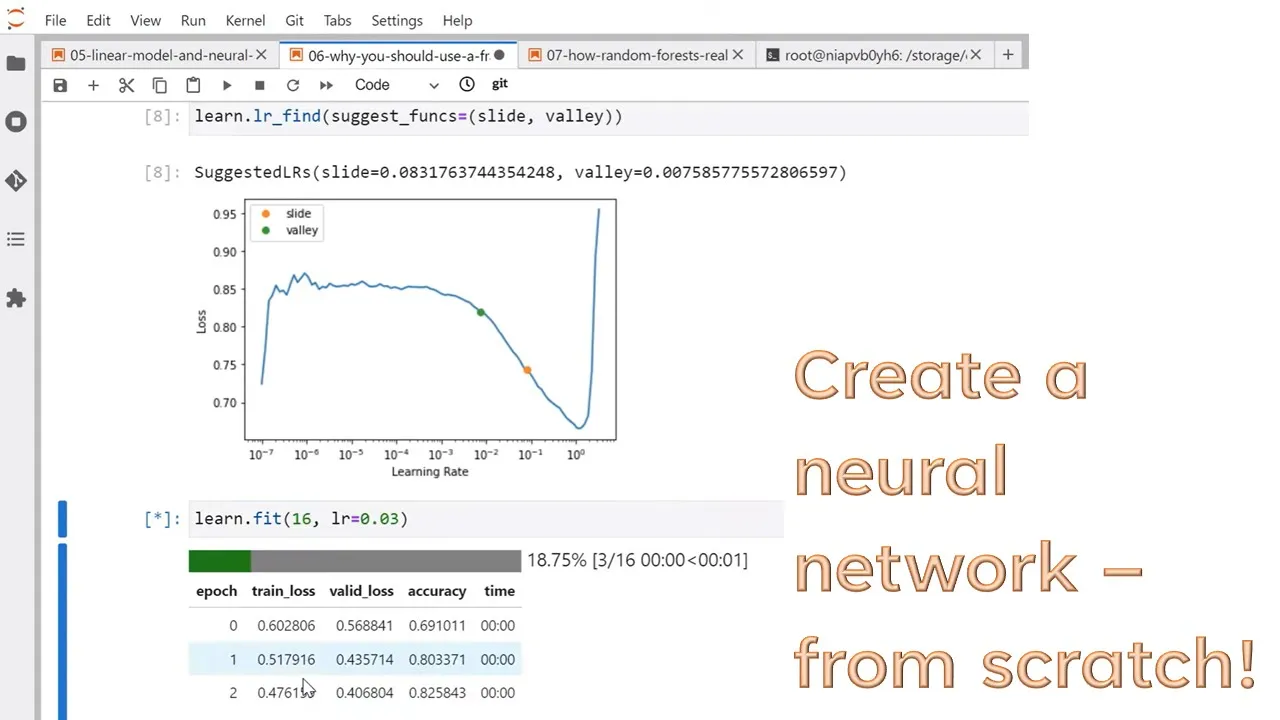
Okay, so this remember is something that contains a model and data. And I want you to put in two hidden layers with 10 units and 10 units, just like we did in our final example. What learning rate should I use? Make a suggestion for me, please. So call it LR find.

You can use this for any fast AI model. Now, what this does is it starts at a learning rate that's very, very small, 10 to the negative seven, and it puts in one batch of data, and it calculates the loss. And then it increases the learning rate slightly and puts through another batch of data.

And it keeps doing that for higher and higher learning rates, and it keeps track of the loss as it increases the learning rate. Just one batch of data at a time. And what happens is for the very small learning rates, nothing happens. But then once you get high enough, the loss starts improving.

And then as it gets higher, it improves faster. Until you make the learning rate so big that it overshoots and then it kills it. And so generally somewhere around here is the learning rate you want. Fast AI has a few different ways of recommending a learning rate. You can look up the docs to see what they mean.

I generally find if you choose slide and valley and pick one between the two, you get a pretty good learning rate. So here we've got about 0.01 and about 0.08. So I picked 0.03. So just run a bunch of epochs, away it goes. This is a bit crazy. After all that, we've ended up exactly the same accuracy as the last two models.

That's just a coincidence, right? I mean, there's nothing particularly about that accuracy. And so at this point, we can now submit that to Kaggle. Now, remember with the linear model, we had to repeat all of the pre-processing steps on the test set in exactly the same way. Don't have to worry about it with fast AI.

And fast AI, I mean, we still have to deal with the fill missing for fair, 'cause that's that. We have to add our feature engineering features. But all the pre-processing, we just have to use this one function called test_dl. That says create a data loader that contains exactly the same pre-processing steps that our learner used.

And that's it, that's all you need. So just 'cause you wanna make sure that your inference time, transformations, pre-processing are exactly the same as a training time. So this is the magic method which does that, just one line of code. And then to get your predictions, you just say get preds and pass in that data loader I just built.

And so then these three lines of code are the same as the previous notebook. And we can take a look at the top and as you can see, there it is. So how did that go? I don't remember. Oh, I didn't say. I think it was again, basically middle of the pack, if I remember correctly.

So one of the nice things about, now that it's so easy to add features and build models is we can experiment with things much more quickly. So I'm gonna show you how easy it is to experiment with, what's often considered a fairly advanced idea, which is called Ensembling. There's lots of ways of doing Ensembling, but basically Ensembling is about creating multiple models and combining their predictions.

And the easiest kind of ensemble to do is just to literally just build multiple models. And so each one is gonna have a different set of randomly initialized coefficients. And therefore each one's gonna end up with a different set of predictions. So I just create a function called Ensemble, which creates a learner, exactly the same as before, fits exactly the same as before and returns the predictions.

And so we'll just use a list comprehension to do that five times. So that's gonna create a set of five predictions. Done. So now we can take all those predictions and stack them together and take the mean over the rows. So that's gonna give us the, well it's actually sorry, the mean over the first dimension.

So the mean over the sets of predictions. And so that will give us the average prediction of our five models. And again, we can turn that into a CSV and submit it to cattle. And that one, I think that went a bit better, let's check. (sniffs) Yeah, okay, so that one actually finally gets into the top 20%, 25% in the competition.

So I mean, not amazing by any means, but you can see that this simple step of creating five independently trained models just starting from different starting points in terms of random coefficients actually improved us from top 50% to top 25%. John. - Is there an argument because you've got a categorical result, you're zero one effectively.

Is there an argument that you might use the mode of the ensemble rather than the numerical mean? - I mean, yes, there's an argument that's been made. And yeah, something I would just try. I generally find it's less good, but not always. And I don't feel like I've got a great intuition as to why.

And I don't feel like I've seen any studies as to why. You could predict, like there's a few, there's at least three things you could do, right? You could take the, is it greater or less than 0.5? Ones and zeros and average them. Or you could take the mode of them.

Or you could take the actual probability predictions and take the average of those and then threshold that. And I've seen examples where certainly both of the different averaging versions, each of them has been better. I don't think I've seen one with the modes better, but that was very popular back in the '90s, so.

Yeah, so it'd be so easy to try. You might as well give it a go. Okay, we don't have time to finish the next notebook, but let's make a start on it. So the next notebook is random forests. How random forests really work. Who here has heard of random forests before?

Nearly everybody, okay. So very popular, developed I think initially in 1999, but gradually improved in popularity during the 2000s. I was like, everybody kind of knew me as Mr. Random Forests for years. I implemented them like a couple of days after the original technical report came out. I was such a fan.

All of my early Kaggle results for random forests. I love them. And I think hopefully you'll see why I'm such a fan of them because they're so elegant and they're almost impossible to mess up. A lot of people will say like, oh, why are you using machine learning? Why don't you use something simple like logistic regression?

And I think like, oh gosh, in industry, I've seen far more examples of people screwing up logistic regression than successfully using logistic regression 'cause it's very, very, very, very difficult to do correctly. You've got to make sure you've got the correct transformations and the correct interactions and the correct outlier handling and blah, blah, blah.

And anything you get wrong, the entire thing falls apart. Random Forests, it's very rare that I've seen somebody screw up a random forest in industry. They're very hard to screw up because they're so resilient and you'll see why. So in this notebook, just by the way, rather than importing numpy and pandas and matplotlib and blah, blah, blah, there's a little handy shortcut, which is if you just import everything from fastai.imports, that imports all the things that you normally want.

So, I mean, it doesn't do anything special, but it's just saved some messing around. So again, we've got our cell here to grab the data. And I'm just gonna do some basic pre-processing here with my fill-in-A for the fair, only needed for the test set, of course. Grab the modes and do the fill-in-A on the modes, take the log fair.

And then I've got a couple of new steps here, which is converting embarked insects into categorical variables. What does that mean? Well, let's just run this on both the data frame and the test data frame. Split things into categories and continuous. And sex is a categorical variable, so let's look at it.

Well, that's interesting. It looks exactly the same as before, male and female, but now it's got a category and it's got a list of categories. What's happened here? Well, what's happened is pandas has made a list of all of the unique values of this field. And behind the scenes, if you look at the cat codes you can see behind the scenes, it's actually turned them into numbers.

It looks up this one into this list to get male, looks up this zero into this list to get female. So when it printed out, it prints out the friendly version, but it stores it as numbers. Now, you'll see in a moment why this is helpful, but a key thing to point out is we're not gonna have to create any dummy variables.

And even that first, second or third class, we're not gonna consider that categorical at all. And you'll see why in a moment. A random forest is an ensemble of trees. A tree is an ensemble of binary splits. And so we're gonna work from the bottom up. We're gonna first work, we're gonna first learn about what is a binary split.

And we're gonna do it by looking at an example. Let's consider what would happen if we took all the passengers on the Titanic and grouped them into males and females. And let's look at two things. The first is let's look at their survival rate. So about 20% survival rate for males and about 75% for females.

And let's look at the histogram. How many of them are there? About twice as many males as females. Consider what would happen if you created the world's simplest model, which was what sex are they? That wouldn't be bad, would it? Because there's a big difference between the males and the females.

A huge difference in survival rate. So if we said, oh, if you're a man, you probably died. If you're a woman, you probably survived. Or not just a man or a boy, so a male or a female. That would be a pretty good model because it's done a good job of splitting it into two groups that have very different survival rates.

This is called a binary split. A binary split is something that splits the rows into two groups, hence binary. Let's talk about another example of a binary split. I'm getting ahead of myself. Before we do that, let's look at what would happen if we used this model. So if we created a model which just looked at sex, how good would it be?

So to figure that out, we first have to split into training and test sets. So let's go ahead and do that. And then let's convert all of our categorical variables into their codes. So we've now got zero, one, two, whatever. We don't have male or female there anymore. And let's also create something that returns the independent variables, which we'll call the X's, and the dependent variable, which we'll call Y.

And so we can now get the X's and the Y for each of the training set and the validation set. And so now let's create some predictions. We'll predict that they survived if their sex is zero, so if they're female. So how good is that model? Remember I told you that to calculate mean absolute error, we can get psychic learn or PyTorch, whatever we do it for us, instead of doing it ourselves.

So just showing you. Here's how you do it just by importing it directly. This is exactly the same as the one we did manually in the last notebook. So that's a 21 and a half percent error. So that's a pretty good model. Could we do better? Well, here's another example.

What about fair? So fair's different to sex because fair is continuous, or log fair, I'll take. But we could still split it into two groups. So here's, for all the people that didn't survive, this is their median fair here, and then this is their quartiles, for bigger fairs and quartiles for smaller fairs.

And here's the median fair for those that survived, and their quartiles. So you can see the median fair for those that survived is higher than the median fair for those that didn't. We can't create a histogram exactly for fair because it's continuous. We could back it into groups to create a histogram, so I guess we can create a histogram, that wasn't true.

What I should say is we could create something better, which is a kernel density plot, which is just like a histogram, but it's like with infinitely small bins. So we can see most people have a log fair of about two. So what if we split on about a bit under three?

That seems to be a point at which there's a difference in survival between people that are greater than or less than that amount. So here's another model, log fair greater than 0.2.7. Much worse, 0.336 versus 0.215. Well, I don't know, maybe is there something better? We could create a little interactive tool.

So what I want is something that can give us a quick score of how good a binary split is, and I want it to be able to work regardless of whether we're dealing with categorical or continuous or whatever data. So I just came up with a simple little way of scoring, which is I said, okay, if you split your data into two groups, a good split would be one in which all of the values of the dependent variable on one side are all pretty much the same, and all of the dependent variables on the other side are all pretty much the same.

For example, if pretty much all the males had the same survival outcome, which didn't survive, and all the females had about the same survival outcome, which is they did survive, that would be a good split. It doesn't just work for categorical variables, it would work if your dependent variable was continuous as well.

You basically want each of your groups within group to be as similar as possible on the dependent variable, and then the other group, you want them to be as similar as possible on the dependent variable. So how similar is all the things in a group? That's the standard deviation.

So what I want to do is basically add the standard deviations of the two groups of the dependent variable, and then if there's a really small standard deviation, but it's a really small group, that's not very interesting, so I'll multiply it by the size. So this is something which says, what's the score for one of my groups, one of my sides?

It's the standard deviation multiplied by how many things are in that group. So the total score is the score for the left-hand side, so all the things in one group, plus the score for the right-hand side, which is, tilde means not, so not left-hand side is right-hand side, and then we'll just take the average of that.

So for example, if we split by sex is greater than or less than 0.5, that'll create two groups, males and females, and that gives us this score, and if we do log fair greater than or less than 2.7, it gives us this score, and lower score is better, so sex is better than log fair.

So now that we've got that, we can use our favorite interact tool to create our little GUI, and so we can say, let's try like, oh, what about this one, can we, oops. Can we find something that's a bit better, 4.8, 0.485? No, not very good. What about P class?

0.468, 0.460. So we can fiddle around with these. We could do the same thing for the categorical variables, so we already know that sex, we can get to 0.407, what about embarked? All right, so it looks like sex might be our best. Well, that was pretty inefficient, right? It would be nice if we could find some automatic way to do all that.

Well, of course we can. For example, if we wanted to find what's the best split point for age, then we just have to create, let's do this again. If we want to find the best split point for age, we could just create a list of all of the unique values of age, and try H1, in turn, and see what score we get if we made a binary split on that level of age.

So here's a list of all of the possible binary split thresholds for age. Let's go through all of them for each of them. Calculate the score. And then NumPy and PyTorch have an argmin function which tells you what index into that list is the smallest. So just to show you, here's the scores.

And zero, one, two, three, four, five, six. Oh, sorry, zero, one, two, three, four, five, six. So apparently that value has the smallest score. So that tells us that for age, the threshold of six would be best. So here's something that just calculates that for a column. It calculates the best split point.

So here's six, right? And it also tells us what the score is at that point, which is 0.478. So now we can just go through and calculates the score for the best split point for each column. And if we do that, we find that the lowest score is six.

So that is how we calculate the best binary split. So we now know that the model that we created earlier, this one, is the best single binary split model we can find. So next week, we're gonna learn how we can recursively do this to create a decision tree, and then do that multiple times to create a random forest.

But before we do, I wanna point something out, which is this ridiculously simple thing, which is find a single binary split in stock is a type of model. It has a name, it's called 1R. And the 1R model, it turned out in a review of machine learning methods in the 90s, turned out to be one of the best, if not the best, machine learning classifiers for a wide range of real world data sets.

So that is to say, don't assume that you have to go complicated. It's not a bad idea to always start creating a baseline of 1R, a decision tree with a single binary split. And in fact, for the titanic competition, that's exactly what we do. If you look at the titanic competition on Kaggle, you'll find that what we did is our sample submission is one that just splits into male versus female.

All right, thanks everybody. Hope you found that interesting, and I will see you next lesson. Bye.