Hello guys! Welcome to my new video on how to code stable diffusion from scratch. And stable diffusion is a model that was introduced last year. I think most of you are already familiar with it. And we will be coding it from scratch using PyTorch only. And as usual my video is going to be quite long, because we will be coding from scratch and at the same time I will be explaining each part that makes up stable diffusion.

So as usual let me introduce you what are the topics that we will discuss and what are the prerequisites for watching this video. So of course we will discuss stable diffusion because we are going to build it from scratch using only PyTorch. So no other libraries will be used except for the tokenizer.

I will describe the maths of the diffusion models as defined in the DDPM paper, but I will simplify it as much as possible. I will show you how classifier-free guidance works and of course we will also implement it, how the text-to-image works, image-to-image and in-painting. Of course to have a very complete view of diffusion models actually we should also introduce the score-based models and all the ODE and SDF theoretical framework.

But most people are not familiar with ordinary differential equations or even stochastic differential equations. So I will not discuss these topics in this video and I'll leave it for future videos. So anyway we will have a complete copy of a stable diffusion, we will be able to generate images using the prompt, also condition on existing images etc.

But for example the samplers based on the Euler method or Runge-Kutta method will not be built in this video. I will make a future video in which I describe these ones. What do I expect you to have as a prerequisite for watching this video? Well first of all it's good that if you have some notion of probability and statistics, so at least you know what is a Gaussian distribution, what is the conditional probability, the marginal probability, the likelihood etc.

Now I don't expect you to have the mathematical formulation in your mind about these concepts, but at least the concepts behind them, so at least what do we mean by conditional probability or what do we mean by marginal probability. Anyway even if you're not very strong with mathematics I will always give a non-mathematics intuition for most concepts.

So even if you don't have this background you will at least understand the concept behind this, some intuition behind this. And of course I expect you to know Python and PyTorch, at least basic level, because we will be coding using Python and PyTorch. And then we will be using a lot the attention mechanism, so if you're not familiar with the transformer model please watch my previous video on the attention and transformer.

And we will also be using a lot of convolutions. So I don't expect you to know how mathematically the convolution layers work, but at least what they do on a practical level in a neural network. Anyway I will also review this while coding. And because this is going to be a long video I will first, because the stable diffusion and the diffusion models in general are quite complex from a mathematical point of view, so we cannot jump directly to the code without explaining what we are going to code and how it works.

The first thing I will do is to give you some background knowledge from a mathematical point of view, but also from a conceptual point of view of how the diffusion models work and how stable diffusion works. And then we will build each part one by one. Of course at the beginning you will have a lot of ideas that are kind of confused because I will give you a lot of new concepts to grasp.

And it's normal that you don't understand everything at the beginning. But don't worry because while coding I will repeat each concept more than once. So while coding you will also get a practical knowledge of what each part is doing and how they interact with each other. So please don't be scared if you don't understand everything in the beginning part of this video.

Later when we start coding it everything will make sense to you. But we need this initial part because otherwise we cannot just jump in the dark and start coding without knowing what we are going to code. So let's start our journey. So what is stable diffusion? Stable diffusion is a model that was introduced in 2022, so last year, at the end of last year I remember, by Confit's group at the Ludwig Maximilian University in Munich, Germany.

And it's open source, the weights, the pre-trained weights can be found on the Internet. And it became very famous because people started doing a lot of stuff and building projects with them and products with them with the stable diffusion. And one of the most simple use of stable diffusion is to do text to image.

So given a prompt we want to generate an image. We will also see how image to image works and also how in-painting works. Image to image means that you already have a picture, for example, of a dog and you want to change it a little bit by using a prompt.

For example, you want to ask the model to add the wings to the dog so that it looks like a flying dog. Or in-painting means that you remove some part of the image. For example, you can remove, I don't know, this part here and you ask the model to replace it with some other part that makes sense, that is coherent with the image.

And we will see also how this works. Let's jump into generative models because diffusion models are generative models. But what is a generative model? Well, a generative model learns a probability distribution of the data such that we can then sample from the distribution to create new instances of the data.

For example, if we have many pictures of cats or dogs or whatever we have, we can train a generative model on it and then we can sample from this distribution to create new images of cats or dogs or whatever. And this is exactly what we do with stable diffusion.

We actually have a lot of images, we train it on a massive amount of images, and then we sample from this distribution to generate new images that don't exist in our training set. But the question may arise in your mind is why do we model data as distributions, as probability distributions?

Well, let me give you an example. Imagine you are a criminal and you want to generate thousands of fake identities. Imagine you also live in a very simple world and each fake identity is made up of variables representing the characteristic of a person. So age and height. Suppose we only have two variables that make up a person.

So it's the age of the person and the height of the person. In my case, I will be using the centimetre for the height. I think the Americans can convert it to feet. And so how do we proceed if we are a criminal with this goal? Well, we can ask the statistics department of the government to give us some statistics about the age and the height of the population.

This information you can easily find online, for example. And then we can sample from this distribution. For example, if we model the age of the population like a Gaussian with the mean of 40 and the variance of 30. OK, these numbers are made up. I don't know if they reflect the reality.

And the height in centimetres is 120 as mean and the variance is 100. We get these two distributions. Then we can sample from these two distributions to generate a fake identity. What does it mean to sample from a distribution? To sample from this kind of distribution means to throw a coin, a very special coin that has a very high chance of falling in this area, a lower chance of falling in this area, an even lower chance of falling in this area and a very nearly zero chance of falling in this area.

So imagine we flip this coin once for the age, for example, and it falls here. So it's quite probable, not very probable, but quite probable. So suppose the age is three and let me write. So the age, let's say, is. Three. And then we toss again this coin and we and the coin falls, let's say here.

So one hundred, let's say, thirty height. One hundred thirty centimetres. So as you can see, the combination of age and height is quite improbable in reality. I mean, no three years old is one metre and thirty centimetres high. I mean, at least not the ones I know. So this combination of age and height is very not plausible.

So to produce plausible pairs, we actually need to model these two variables. So the age and height, not as independent variables and sample from each of them independently, but as a joint distribution. And usually we represent the joint distribution like this, where each combination of age and height has a probability score associated with it.

And from this distribution, we only sample using one coin. And for example, this coin will have a very high probability with very high chance will fall in this area, with less chance will fall in this area and very close to zero chance of falling in this area. Suppose we throw the coin and it ends up in this area to get to the corresponding.

Suppose this is the age and this is the height to get to the corresponding age and height. We just need to do like this. And suppose these are actually the real height and the real height. Now the numbers here are actually do not match, but you got the idea that to model something, we need a joint distribution over all the variables.

And this is actually what we do also with our images. With our images, we create a very complex distribution in which, for example, each pixel is a distribution and the entirety of all the pixels are one big joint distribution. And once we have a joint distribution, we can do a lot of interesting things.

For example, we can marginalize. So, for example, imagine we have a joint distribution over the age and the height. So let's call the age X and let's call the height, let's say Y. So if we have a joint distribution, which means having P of X and Y, which is defined for each combination of X and Y, we can always calculate P of X.

So the probability of over the single variable by marginalizing over the other. So as the integral of P of X and Y and the Y. And this is how we marginalize, which means marginalizing over all the possible Y that we can have. And then we can also calculate the probability, the conditional probability.

For example, we can say that the probability, what is the probability of the age being, let's say, from 0 to 3, given that the height is more than 1 meter. So something like this. We can do this kind of queries by using the conditional probability. So this is actually what we do with the generative model.

We model our data as a very big joint distribution. And then we learn the parameters of this distribution, because it's a very complex distribution. So we let the neural network learn the parameters of this distribution. And our goal, of course, is to learn this very complex distribution and then sample from it to generate new data, just like the criminal before wanted to generate new fake identities by modeling the very complex distribution that represents the identity of a person.

In our case, we will model our system as a joint distribution by including also some latent variables. So let me describe. As you probably are familiar with the diffusion models, we have two processes. One is called the forward process and one is called the reverse process. The forward process means that we have our initial image that we will call X0, so this here, and we add noise to it to get another image that is the same as the previous one, but with some noise on top of it.

Then we take this image, which has a little noise, and we generate a new image that is same as the previous one, but with even more noise. So as you can see, this one has even more noise, and so on, so on, so on, until we arrive to the last latent variable called Zt, where t is equal to 1000, when it becomes completely noise, pure noise, like N0,1, actually N0i, because we are in the multivariate world.

And our goal, actually, is to... this process, this forward process is fixed. So we define how to build the noisified version of each image given the previous one, so we know how to add noise, and we have a specific formula, an analytical formula, on how to add noise to an image.

The problem is, we don't have the analytical formula to reverse this process, so we don't know how to take this one and just remove noise. There is no closed formula on how to do it, so we learn, we train a neural network to do this inverse process, to remove noise from something that has noise.

And if you think about it, it is quite easy to add noise to something than it is to remove noise from something. That's why we are using a neural network for this purpose. Now we need to go inside, of course, of the math, because we will be using it not only to write the code, but also to write the sampler.

And in the sampler, it's all about mathematics. And I will try to simplify it as much as possible, so don't be scared. So let's start. Okay, this is from the DDPM paper, so the Noising Diffusion Probabilistic Models, from Ho in 2020. And here we have two processes. The first is the forward process, which means that given the original image, how can I generate the noisified version of this image at time step t?

In this case, actually, this is the joint distribution. Let's look at this one here. This means if I have the image at time step t minus one, how can I get the next time step, so the more noisified version of this image? Well, we define it as a Gaussian distribution centered, so the mean centered on the previous one, and the variance defined by this beta parameter here.

This beta parameter here is decided by us, and it means how much noise we want to add at every step of this noisification process. This is also known as the Markov chain of noisification, because each variable is conditioned on the previous one. So to get xt, we need to have xt minus one.

And as you can see from here, we start from x0, we go to x1. Here I call it z1 to differentiate it, but x1 actually is equal to z1. So x0 is the original image, and all the next x are noisy versions, with xt being the most noisy. So this is called the Markov chain of noisification, and we can do it like this.

So it's defined by us as a process, which is a series of Gaussians that add noise. There is an interesting formula here. This is a closed loop, closed formula, to go from the original image to any image at time step t, without calculating all the intermediate images, using this particular parametrization.

So we can go from the image, original image, to the image at time step t, by sampling from this distribution, by defining the distribution like this. So with this mean and with this variance. This mean here depends on a parameter, alpha, alpha bar, which is actually depending on beta.

So it's something that we know, there is nothing we have to learn. And also the variance actually depends on alpha, which is defined as in function of beta. So beta is also something we know, so there is no parameters to learn here. Now let's look at the reverse process.

The reverse process means that we have something noisy, and we want to get something less noisy. So we want to remove noise. And we also define it as a Gaussian, with a mean, mu theta, and a variance, sigma theta. Now, this mean and this variance are not known to us.

We have to learn them. And we will use a neural network to learn these two parameters. Actually, the variance, we will also set this at fixed. We will parameterize it in such a way that this variance actually is fixed. So we hypothesize, we already know the variance. And we let the network learn only the mean of this distribution.

So to rehearse, we have a forward process that adds noise. And we know everything about this process. We know how to add noise. We have a reverse process that we don't know how to denoise. So we let a network learn the parameters on how to denoise it. And OK, now that we have defined these two processes, how do we actually train a model to do it?

Because as you remember, our initial goal is actually to learn a probability distribution over our data set. And so this quantity here. But unlike before, when we could marginalize, for example, in the case of the criminal who want to generate identities, we could marginalize over all the variables. Here we cannot marginalize.

Because we need to marginalize over x1, x2, xt, x4, up to xt. So over a lot of variables. And to calculate this integral means to calculate it over all the possible x1. And over all the possible x2, et cetera. So it's a very complex calculation that is computationally intractable, we say.

It means that it's theoretically possible. But practically, it will take forever. So we cannot use this route here. So what can we do? We want to learn this quantity here. So we want to learn the parameter theta of this to maximize the likelihood we can see here. What we did is we found a lower bound for this quantity here.

So the quantity, the likelihood. And this lower bound is called the elbow. And if we maximize the lower bound, it will also maximize the likelihood. So let me give you a parallel example on what it means to maximize the lower bound. For example, imagine you have a company. And your company has some revenue.

And usually, the revenue is more than or equal to the sales of your company. So you have some revenue coming from sales. Maybe you also have some revenue coming from interest that you get from your bank, et cetera. But we can for sure say that the revenue of your company is more than or equal to the sales of your company.

So if you want to maximize your revenue, you can maximize your sales, for example, which is a lower bound over your revenue. So if we maximize the sales, we will also maximize the revenue. And this is the idea here. But how do we do it on a practical level?

Well, this is the training code for the DDPM diffusion models as defined by the DDPM paper. And basically, the idea is after we get the elbow, we can parameterize the loss function as this. Which says that we need to learn-- we need to train a network called epsilon theta.

That given a noisy image-- so this formula here means the noisy image at time step t and the time step at which the noise was added, the network has to predict how much noise is in the image, the noisified image. And if we do gradient descent over this loss function here, we will maximize the elbow.

And at the same time, we will also maximize the log likelihood of our data. And this is how we train these kind of networks. Now, I know that this is a lot of concept that you have to grasp. So don't worry. For now, just remember that there is a forward process and there is a reverse process.

And to train this network to do the reverse process, we need to train a network to detect how much noise is in a noisified version of the image at time step t. Let me show you how do we-- once we have this network that has already been trained, how do we actually sample to generate new data?

So let's go here. Let's go here. So how do we generate new data? Suppose we already have a network that was trained for detecting how much noise is in there. And what we do is we start from complete noise. And then we ask the network to detect how much noise is in there.

We remove this noise. And then we ask the network again how much noise is in there. And we remove it. And then we ask the network how much noise is there. OK, remove it. Then how much noise is here? OK, remove it, et cetera, et cetera. Until we reach this step, then here we will have something new.

So if we start from pure noise and we do this reverse process many times, we will end up with something new. And this is the idea behind this generative model. Now that we know how to generate new data starting from pure noise, we also want to be able to control this denoisification process so we can generate images of something that we want.

I mean, how can we tell the model to generate a picture of a cat or a picture of a dog or a picture of a house by starting from pure noise? Because as of now, by starting from pure noise and keep denoising, we will generate a new image, of course.

But it's not like we can control which new image will be generated. So we need to find a way to tell the model what we want in this generational process. And the idea is that we start from pure noise. And during this chain of removing noise, so denoisification, we introduce a signal.

Let's call it prompt. Prompt. Or it can also be called the conditioning signal. Or it can also be called the context. Anyway, they are the same concept. In which we influence the model into how to remove the noise so that the output will move towards what we want. To understand how this works, let's review again how the training of this kind of networks works.

Because this is very important for us. To learn how the training of this kind of network goes, so that we can introduce the prompt. Let's go back. Okay, as I told you before, our final goal is to model a distribution, theta, p of theta, such that we maximize the likelihood of our data.

And to learn this distribution, we maximize the ELBO, so the lower bound. But how do we maximize the ELBO? We minimize this loss, minimize this loss here. So by minimizing this loss, we maximize the ELBO, which in turn learns this distribution here. Because this ELBO here is the lower bound for the likelihood of our data distribution here.

And what is this loss function? Loss function here indicates that we need to create a model, epsilon theta, such that if we give this model a noisified image at a particular noise level, and we also tell him what noise level we included in this image, the network has to predict how much noise is there.

So this epsilon is how much noise we have added. And we can do a gradient descent on this training loop. This way we will learn a distribution of our data. But as you can see, this distribution doesn't include anything that tells the model what is a cat, or what is a dog, or what is a house.

The model is just learning how to generate pictures that make sense, that are similar to our initial training data. But they don't know what is the relationship between that picture and the prompt. So one idea could be, OK, can we learn a joint distribution of our initial data, so all the images, and the conditioning signal, so the prompt?

Well, this is also something that we don't want, because we want to actually learn this distribution, so that we can sample and generate new data. We don't want to learn the joint distribution that will be too much influenced by the context, and the model may not learn the generative process of the data.

So our final goal is always this one. But we also want to find some how to condition this model into building something that we want. And the idea is that we modify this unit, so this model here, epsilon theta, will be built using, let me show you, this unit model here.

This unit will receive as input an image that is noisified, so for example, a cat, with a particular noise level, and we also tell him what is the noise level that we added to this cat, and we give them both to the input of the unit, and the unit has to predict how much noise is there.

This is the job of the unit. What if we introduce also the prompt signal here, so the conditioning signal here, so the prompt? This way, if we tell the model, can you remove noise from this image, which has this quantity of noise, and I am also telling you that it's a cat, so the model has more information on how to remove the noise.

Yes, the model can learn this way, how to remove noise into building something that is more closer to the prompt. This will make the model conditioned, it means that it will act like a conditioned model, so we need to tell the model what is the condition that we want, so that the model can remove the noise in that particular way, moving the output towards that particular prompt.

But at the same time, when we train the model, instead of only giving images along with the prompt, we can also sometimes, with a probability, let's say 50%, not give any prompt and let the model remove the noise without telling him anything about the prompt. So we just give him a bunch of zero when we give him the input.

This way, the model will learn to act both as a conditioned model and also as a conditioned model, so the model will learn to pay attention to the prompt and also to not pay attention to the prompt. And what is the advantage of this? Is that we can, once when we want to generate a new picture, we can do two steps.

In the first one, suppose you want to generate a picture of a cat, we can do like this. Let me delete first of all. Okay, we can do the first step. So let's call it step one. And we can start with pure noise, because as I told you before, to generate a new image, we start from pure noise.

We indicate the model what is the noise level. So at the beginning, it will be t equal to 1000, so maximum noise level. And we tell the model that we want a cat. We give this as input to the unit. The unit will predict some noise that we need to remove in order to move the image towards what we want as output.

So a cat. And this is our output one. Let's call it output one. Then we do another step. So let me delete this one. Then we do another step. Let's call it step two. And again, we give the same input noise as before, the same time step as the noise level.

So it's the same noise with the same noise level, but we don't give any prompt. This way, the model will build some output. Let's call it out two, which is how to remove the noise to generate something. We don't know what, but to generate something that belongs to our data distribution.

And then we combine these two output in such a way that we can decide how much we want the output to be closer to the prompt or not. This is called classifier-free guidance. So this approach here is called classifier-free guidance. I will not tell you why it's called classifier-free guidance, because otherwise I need to introduce the classifier guidance.

And to talk about the classifier guidance, I need to introduce the score-based models to understand why it's called like this. But the idea is this, that we train a model that, when we train it, sometimes we give it the prompt and sometimes we don't give it the prompt, so that the model learns to ignore the prompt, but also to pay attention to the prompt.

And when we sample from this model, we do two steps. First time, we give him the prompt of what we want. And the second time, we give the same noise, but without the prompt of what we want. And then we combine the two output, conditioned and unconditioned, linearly with a weight that indicates how much we want the output to be closer to our condition, to our prompt.

The higher this value, the more the output will resemble our prompt. The lower this value, the less it will resemble our prompt. And this is the idea behind classifier-free guidance. To give the prompt, actually we will give, we need to give some kind of embedding to the, so the model needs to understand this prompt.

To understand the prompt, the model needs some kind of embedding. Embedding means that we need some vectors that represent the meaning of the prompt. And this embedding are extracted using the CLIP text encoder. So before talking about the text encoder, let's talk about CLIP. So CLIP was a model built by OpenAI that allowed to connect text with images.

And the text, basically, they took a bunch of images. So for example, this picture and its description. Then they took another image along with its description. So the image one is associated with the text number one, which is the description of the image one. Then the image two has the description number two.

The image three has the text number three, which is the description of the image three, et cetera, et cetera. They built this matrix, you can see here, which is made up of the dot products of the embedding of the first image multiplied with all the possible captions here. So the image one with the text one.

Image one with the text two. Image one with the text three, et cetera. Then image two with the text one. Image two with the text two, et cetera. How they train it? Basically, we know that the correspondence between image and the text is on the diagonal because the image one is associated with the text one.

Image two is associated with the text two. Image three is associated with the text three. So how they train it? Basically, they said they built a loss function that they want this diagonal to have the maximum value and all the other numbers here to be zero because they are not matching.

They are not the corresponding description of these images. In this way, the model learned how to combine the description of an image with the image itself. And what we do in stable diffusion is that we take this text encoder here, so only this part of this clip, to encode our prompt to get some embeddings.

And these embeddings are then used as conditioning signal for our unit to denoise the image into what we want. Okay, there is another thing that we need to understand. So as I said before, we have a forward process that adds noise to the image. Then we have a reverse process that removes noise from the image.

And this reverse process can be conditioned by using the classifier-free guidance. And this reverse process means that we need to do many steps of denoisification to arrive to the image, to the new image. And this also means that each of these steps involves going through the unit with a noisified image and getting as output the amount of noise present in this image.

But if the image is very big, so suppose this image here is 512 multiplied by 512, it means every time on the unit, we will have a very big matrix that needs to go through this unit. And this may be very slow, because it's a very big matrix of data that the unit has to work on.

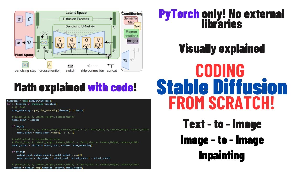
What if we could somehow compress this image into something smaller, so that each step through the unit takes less time? Well, the idea is that yes, we can compress this image with something that is called the variational autoencoder. Let's see how the variational autoencoder works. Okay, the stable diffusion is actually known as a latent diffusion model, because what we learn is not the data probability distribution Px of our data, but we learn the latent representation of the data using a variational autoencoder.

So basically we compress our data, so let's go back, we compress our data into something smaller, and then we learn the noisification process using this compressed version of the data, not the original data. And then we can decompress it to build the original data. Let me show you actually how it works on a practical level.

So imagine you have some data and you want to send it to your friend over the internet. What do you do? You can send the original file or you can send the zipped file. So you can zip the file, maybe with WinZip, for example, and then you send the file to your friend and the friend can unzip it after receiving and rebuild the original data.

This is exactly the job of the autoencoder. The autoencoder is a network that given an image, for example, will, after passing through the encoder, will transform into a vector which has a dimension that is much smaller than the original image. And if we use this vector and run it through the decoder, it will build the original image back.

And we can do it for many images and each of them will have a representation in this. This is called a code corresponding to each image. Now, the problem with autoencoder is that the code learned by this model doesn't make any sense from a semantic point of view. So the code associated with the cat, for example, may be very similar to the code associated with pizza, for example, or the code associated with a building.

So there is no semantic relationship between these codes. And to overcome this limitation of the autoencoder, we introduce the variational autoencoder, in which we learn to kind of compress the data, but at the same time, this data is distributed according to a multivariate distribution, which most of the times is a Gaussian.

And we learn the mean and the sigma of this distribution, this very complex distribution here. And given the latent representation, we can always pass it through the decoder to rebuild the original data. And this is the idea that we use also in stable diffusion. Now we can finally combine all these things that we have seen together to see what is the architecture of the stable diffusion.

So let's start with how the text-to-image works. Now, imagine text-to-image basically works like this. Imagine you want to generate a picture of a dog with glasses. So you start, of course, with a prompt, a dog with glasses. And then what do we do? We sample some noise here, some noise from the N01.

We encode it with our variational autoencoder. This will give us a latent representation of this noise. Let's call it Z. This is, of course, a pure noise, but has been compressed by the encoder. And then we send it to the unit. The goal of the unit is to detect how much noise is there.

And also, because to the unit, we also give the conditioning signal, the unit has to detect the noise, what noise we need to remove to make it into a picture that follows the prompt, so into a picture of a dog. So the unit, we pass it through the unit along with the time step, initial time step, so 1,000.

And the unit will detect at the output here how much noise is there. Our scheduler, we will see later what is the scheduler, will remove this noise and then send it again to the unit for the second step of denoisification. And again, we send the time step, which is in this case not 1,000, but 980, for example, because we skipped some steps.

And then we again, with the noise, we detect how much noise is there. The scheduler will remove this noise and again send it back. And we do many times this. We keep doing this denoisification for many steps until there is no more noise present in the image. And after we have finished this loop of steps, we get the output Z prime, which is still a latent because this unit only works with the latent representation of the data, not with the original data.

We pass it through the decoder to obtain the output image. And this is why this is called a latent diffusion model because the unit, so the denoisification process, always works with the latent representation of the data. And this is how we generate text to image. We can do the same thing for image to image.

Image to image means that I have, for example, the picture of a dog and I want to modify this image into something else by using a prompt. For example, I want the model to add glasses to this dog so I can give the input image here. And then I say a dog with glasses and hopefully the model will add glasses to this dog.

How does it work? We encode the image with the encoder of the variational autoencoder and we get the latent representation of our image. Then we add noise to this latent because the unit, as we saw before, his job is to denoise an image. But of course, we need to have some noise to denoise.

So we add noise to this image and the amount of noise that we add to this image, so this starting image here, indicates how much freedom the unit has into building the output image. Because the more noise we add, the more the unit has freedom to alter the image.

But the less noise we add, the less freedom the model has to alter the image because it cannot change radically. If we start from pure noise, the unit can do anything it wants. But if we start with less noise, the unit is forced to modify just a little bit the output image.

So the amount of noise that we start from indicates how much we want the model to pay attention to the initial image here. And then we give the prompt. For many steps, we keep denoising, denoising, denoising, denoising. And after there is no more noise, we take this latent representation, we pass it through the decoder and we get the output image here.

And this is how image-to-image works. Now let's go to the last part, which is how in-painting works. In-painting works similar way to the image-to-image, but with a mask. So in-painting means, first of all, that we have an image and we want to cut some part of this image, for example, the legs of this dog and we want the model to generate new legs for this dog that are maybe a little different.

So as you can see, these feet here are a little different from the legs of the dog here. So what we do is, we start from our initial image of the dog. We pass it through the encoder. It becomes a latent representation. We add some noise to this latent representation.

We give some prompt to tell the model what we want the model to generate. So I just say a dog running because I want to generate new legs for this dog. And then we pass the noisified input to the unit. The unit will produce an output here for the first time step.

But then, of course, nobody told the model to only predict this area. The model, of course, here at the output predicted and modified the noise all the image. But we take this output here and we don't care what the noise predicted for this area of the image. The area that we already know.

We replace it with the image that we already know. And we pass it again through the unit. Basically, what we do is, at every step, at every output of the unit, we replace the areas that are already known with the areas of the original image. So, basically, to fool the model into believing that it was the model itself that came up with these details of the image, not us.

So every time here in this area, before we send it back to the unit here, here we combine the output of the unit with the existing image by replacing whatever output the unit gave us for this area here with what is the original image. And then we give it back to the unit and we keep doing it.

This way the model will only be able to work on this area here because this is the one we never replace in the output of the unit. And then after there is no more noise, we take the output, we send it to the decoder and then it will build the image we can see here.

Okay, this is how the stable diffusion works from an architecture point of view. I know it has been a long journey. I had to introduce many concepts but it's very important that we know these concepts before we start building the unit because otherwise we don't even know how to start building the stable diffusion.

Here we are finally coding our stable diffusion. And the first thing that we will code is the variational autoencoder because it's external to the unit, so it's external to the diffusion model, so the one that will detect, will predict how much noise is present in the image. And let's review it actually.

Let's review the architecture and let me go to this slide here. Okay, oops. This one here. Okay, the first thing that we will build is this part here. The encoder and the decoder of our variational autoencoder. The job of the encoder and the decoder of the variational autoencoder is to encode an image or noise into a compressed version of the image or the noise itself such that then we can take this latent and run it through the unit.

And then after the last step of the noisification we take this compressed version or latent and we pass it through the decoder and to get the original, the output image, not the original. And so the encoder, actually his job is to reduce the dimension of the data into a smaller data, into the data with the smaller dimension.

And the idea is very similar to the one of the unit. So we start with a picture that is very big and at each step there are multiple levels. We keep reducing the size of the image but at the same time we keep increasing the features of the image.

What does it mean? That initially each pixel of the image will be represented by three channels. So red, green and blue RGB. At each step by using convolutions we will reduce the size of the image but at the same time we will increase the number of features that each pixel represents.

So each pixel will be represented not by three channels but maybe by more channels. This means that each pixel will actually capture more data. More data of the area to which that pixel belongs. And this is thanks to the convolutions. But I will show you later with an animation.

So let's start building. The first thing we do is open Visual Studio. And we create three folders. The first is called data. And later we download the pre-trained weights that you can also find on my GitHub. Another folder called images in which we put images as input and output.

And then another folder called SD which is our module. Let's create two files. One called encoder.py and one called decoder.py. These are the encoder and the decoder of our variational autoencoder. Let's start with the encoder. And the encoder is quite simple. So let's start by importing Torch and all the other stuff.

Let me also select the interpreter. Okay. Then we need to import two other blocks that we will define later in the decoder. Let's call them for now port VAE attention block. And this is the port VAE attention block. And this is the port VAE attention block. And this is the port VAE attention block.

And this is the port VAE attention block. And VAE residual block. For those who are familiar with computer vision models, the residual block is very similar to the residual block that is used in the ResNet. So later you will see the structure. It's very similar. But if those who are not familiar, don't worry, I will explain it later.

So let's start building this encoder. And this will inherit from the sequential module which means basically our encoder is a sequence of modules, submodules. Okay. It's a sequence of submodules in which each module is something that reduces the dimension of the data, but at the same time increases its number of features.

I will write the blocks one by one. And as soon as we encounter a block that we didn't define, we go to define it. And then we define also the shapes. So the first thing we do, just like in the unit, is we define a convolution. Convolution 2D. Initially, our image will have three channels.

And we convert it to 128 channels with a kernel size of 3 and a padding of 1. For those who are not familiar with convolutions, let's go have a look at how convolutions work. Here. Here we can see that a convolution, basically, it's a kernel. So it's made of a matrix of a size that we can decide, which is defined by the parameter kernel size, which is run through the image as in the following animation.

So block by block, as you can see. And at each block, each of the pixel below the kernel is multiplied by the value of the kernel in that position. So in this, for example, this pixel here, which is in position, let's call the, let's say this one here. So the first row and the first column is multiplied by this red value of the kernel.

The second column, first row, is multiplied by the green value of the kernel. And then all of these multiplications are summed up to produce one output. So this output here comes from four multiplications that we do in this area, each one with the corresponding number of the kernel. This way, basically, by running this kernel through the image, we capture local information about the image.

And this pixel here combines somehow the information of four pixels, not only one. And that's it. Then we can also increase the kernel size, for example. And the kernel size, increasing the kernel means that we capture more global information. So each pixel represents the information of more pixel from the original picture.

So the output is smaller. And then we can introduce, for example, the stride, which means that we don't do it every successive pixel, but we skip some pixels, as you can see here. So we skip every second pixel here. And if the number is, the kernel size is even and the input size is odd, we will also never touch, for example, here, the border, as you can see.

We can also implement a dilation, which means that it becomes, with the same kernel size, the information becomes even more global because we don't watch consecutive pixel, but we skip some pixels, et cetera, et cetera. So the kernels, basically, the convolutions allow us to capture information from a local area of the picture, of the image, and combine it using a kernel.

And this is the idea behind convolutions. So this convolution here, for example, will start with our, okay, let's define some shapes. Our variational autoencoder, so the encoder of the variational autoencoder will start with batch size and three channels. Let's define it as channel. Then this image will have a height and the width, which will be 512 by 512, as we will see later.

And this convolution will convert it into batch size 128 features with the same height and the same width. Why, in this case, the height and the width doesn't change? Because even if we have a kernel size of size three, because we add padding, basically, we add something to the right side, something to the top side, something to the bottom and the left of the image.

So the image with the padding becomes bigger, but then the output of the convolution makes it smaller and matches the original size of the image. This is the reason we have the padding here. But we will see later that with the next blocks, the image size will start becoming smaller.

The next block is called the residual block. And VAE residual block, which is from 128 channels to 128 channels. This is a combination, this residual block is a combination of convolutions and normalization. So it's just a bunch of convolutions that we will define later. And this one indicates how many input channels we have and how many output channels we have.

And the residual block will not change the size of the image. So we define it. So our input image is 128. So batch size 128 height and width. And it becomes, it remains the same basically. Oops! Okay, we have another one. Another residual block with the same transformation. Then we have another convolution.

And this time the convolution will change the size of the image. And we will see why. So we have a convolution. To the 128 to 128. Because the output channels of the last block is 128. So the input channel is 128. The output is 128. The kernel size is 3.

The stride is 2. And the padding is 0. This will basically introduce kernel size 3, stride 2. Let's watch. So imagine the batch size is 6 by 6. Kernel size is 3. Stride is 2 without the deletion. And this is the output. Let me make it bigger. Okay, something.

Yeah. So as you can see, with the stride of 2... Need to make it... Okay, with the stride of 2 and the kernel size of 3. This is the behavior. So we skip every 2 pixels before calculating the output. And this makes the output smaller than the input. Because of this stride.

And also because of the kernel size. And we don't have any padding. So this transformation here will have the following shapes. So we are starting from batch size. 128. Height, width. So the original height and the width of the input image. But this time it will become batch size.

128. The height will become half. And the width will become half. Etc. Then we have two more residual blocks. With the same... Same as before. But this time by increasing the number of features. And also here we don't increase any. Here by increasing the feature means that we don't increase the size of the image.

Or we reduce the size of the image. We just increase the number of features. So this one becomes 256. And here we start from... Oops 256 and we remain 256. Now you may be confused of why we are doing all of this. Okay the idea is we start with the initial image.

And we keep decreasing the size of the image. So later you will see that the image will become divided by 4, divided by 8. But at the same time we keep increasing the features. So each pixel represents more information. But the number of pixels is diminishing. Is reducing at every step.

So let's go forward. Then we have another convolution. And this time the size will become divided by 4. And the convolution is... Let me copy this one. 256 by 256. Because the previous output is 256. The kernel size is 3. The stride is 2 and the padding is 0.

So just like before. Also in this case the size of the image will become half of what is it now. So the image is already divided by 2. So it will become divided by 4 now. Then we have another residual block. In which we increase the number of features.

This time from 256 to 512. So we start from 256 and the image is divided by 4. And we go to 512. And the image size doesn't change. Then we have another one. From 512 to 512. In this case... Oops. We will see later what is the residual block.

But the residual block you have to think of it as just a convolution with a normalization. We will see later. And this one is 512. And that goes into 512. And then we have another convolution that will make it even smaller. So let's copy this convolution here. This one will go from 512 to 512.

The same kernel size and the same stride and the same padding as before. So the image will become even smaller. So our last dimension was this. Let me copy it. So we start with an image that is 512. 4 times smaller than the original image. And with the 4 times smaller width it will become 8 times smaller.

And that's it. And then we have residual blocks also here. We have three of them in this case. Let me copy. One, two, three. I just write the one for the last one. So anyway the size, the shape changes here. It doesn't change the shape of the image or the number of features.

So here we are going from divide by 8 and 512 here. 512. And we go to same dimension. 512. Divide by 8 and divide by 8. Then we have an attention block. And later we will see what is the attention block. Basically it will run a self-attention over each pixel.

So each pixel will become kind of, as you remember, the attention is a way to relate tokens to each other in a sentence. So if we have an image made of pixels, the attention can be thought of as a sequence of pixels and the attention as a way to relate the pixel to each other.

So this is the goal of the attention block. And because this way each pixel is related to each other, is not independent from each other. Even if the convolution already actually relates close pixels to each other, but the attention will be global. So even the last pixel can be related to the first pixel.

This is the goal of the attention block. And also in this case we don't reduce the size because the attention is, the transformer's attention, is a sequence-to-sequence model. So we don't reduce the size of the sequence. And the image remains the same. Finally, we have another residual block. Let's...

Let me copy here. Also no change in shape or size of the image. Then we have a normalization. And we will see what is this normalization. It's the group normalization, which also doesn't change the size. Just like any normalization, by the way. With the number of groups being 32 and the number of channels being 512, because it's the number of features.

Finally, we have an activation function called the CELU. The CELU is a function... Okay, it's derived from the sigmoid linear unit. And it's a function just like the RELU. There is nothing special. They just saw that this one works better for this kind of application. But there is no particular reason to choose one over another, except that they thought that practically this one works fine for this kind of models.

And if you watch my previous video about LAMA, for example, in which we analyzed why they chose the ZWIGLU function. If you read the paper, at the end of the paper, they say that there is no particular reason they chose the ZWIGLU. They just saw that practically it works better.

I mean, it's very difficult to describe why activation function works better than the others. So this is why they use the CELU here, because practically it works well. Now, we have another two convolutions. And then we are done with the encoder. Convolution, 512, 8, kernel size, and then padding.

This will not change the size of the model. Because just like before, we have the kernel size as 3. But we have the padding that compensates for the reduction given by the kernel size. But we are decreasing the number of features. And this is the bottleneck of the encoder.

And I will show you later on the architecture what is the bottleneck. And finally, we have another convolution. Which is 8 by 8 with kernel size equal to 1. And the padding is equal to 0. Which also doesn't change the size of the image. Because if you watch here, if you have a kernel size of 1, it means that each, without stride, each kernel basically is running over each pixel.

So each output actually captures the information of only one pixel. So the output has the same dimension as the input. And this is why here also we don't change the... But here we need to change the number of... It becomes 8. And here from 8 to 8. And this is the list of modules that will make up our encoder.

Before building the residual block and the attention block, so this attention block, let's write the forward method and then we build the residual block. So this is the init. Define it like this. Let me review it if it's correct. Okay, yeah. Now let's define the forward method. x is the image for which we want to encode.

So it's a tensor. Torch.tensor. And the noise, we need some noise. And later I will show you why we need some noise. That has the same size as the output of the encoder. This returns a tensor. Okay, our input x will be of size patch size with some channels.

Initially it will be 3 because it's an image. Height and width which will be 512 by 512. And then some noise. This noise has the same size as the output of the encoder. And we will see that it's jelly patch size. Then output channels. Height divided by 8 and width divided by 8.

Then we just run sequentially all of these modules. And then there is one little thing here that in the convolutions that have the stride, we need to apply a special embedding. And I will show you why and how it works. So if the module has a stride attribute and it's equal to 2 2, which basically means this convolution here, this convolution here and this convolution here, we don't apply the padding here because the padding here is applied to the top of the image, bottom, left and right.

But we want to do an asymmetrical padding so we do it manually. And this is applied like this. F.padding. Basically this says can you add a layer of pixels on the right side of the image and on the bottom side of the image only? Because when you apply the padding, it's padding left, padding right, padding top, padding bottom.

This means add a layer of pixels in the right side of the image and on the top side of the image. And this is asymmetrical padding. And then if we apply it only for these convolutions that have the stride equal to 2. And then x is equal to module of x.

OK, now you may be wondering why are we building this kind of structure? Why it's made like this? OK, usually in deep learning communities, especially during research, we don't reinvent the wheel every time. So the people who made the stable diffusion, but also the people before them, every time we want to use a model, we check what models similar to the one we want to build are already out there and they are working fine.

So very probably the people who built stable diffusion, they saw that a model like this is working very well for some previous project as a variational autoencoder. They just modified it a little bit and kept it like it. So for most choices, actually, there is no reason. There is a historical reason, because it worked well in practice.

And we know that convolutions work well in practice for image segmentation, for example, or anything related to computer vision. And this is why they made the model like this. So most encoders actually work like this, that we reduce the size of the image, but each we keep increasing the features of the image, the channels, the number of channels of the image.

So the number of pixels becomes smaller, but each pixel is represented by more than three channels. So more channels at every step. Now, what we do is here we are running our image into sequentially, in one by one, through all of these modules here. So first through this convolution, then through this residual block, which is also some convolutions, then this residual block, then again convolution, convolution, convolution, until we run it through this attention block and et cetera.

This will transform the image into something smaller, so a compressed version of the image. But as I showed you before, this is not an autoencoder. This is a variational autoencoder. So the variational autoencoder, let me show you again the picture here. We are not learning how to compress data.

We are learning a latent space. And this latent space are the parameters of a multivariate Gaussian distribution. So actually, the variational autoencoder is trained to learn the mu and the sigma, so the mean and the variance of this distribution. And this is actually what we will get from the output of this variational autoencoder, not directly the compressed image.

And if this is not clear, guys, I made a previous video about the variational autoencoder, in which I show you also why the history of why we do it like this, all the reparameterization trick, et cetera. But for now, just remember that this is not just a compressed version of the image, it's actually a distribution.

And then we can sample from this distribution. And I will show you how. So the output of the variational autoencoder is actually the mean and the variance. And actually, it's actually not the variance, but the log variance. So the mean and the log variance is equal to torch.chunk(x2, dimension equal 1).

We will see also what is the chunk function. So I will show you. So this basically converts batch size, 8 channels, height, height divided by 8, width divided by 8, which is the output of the last layer of this encoder. So this one. And we divide it into two tensors.

So this chunk basically means divide it into two tensors along this dimension. So along this dimension, it will become two tensors of size, along this dimension of size 4. So two tensors of shape, batch size 4, then height divided by 8, and width divided by 8. And this basically, the output of this actually represents the mean and the variance.

And what we do, we don't want the log variance, we want the variance actually. So to transform the log variance into variance, we do the exponentiation. So the first thing actually we also need to do is to clamp this variance, because otherwise it will become very small. So clamping means that if the variance is too small or too big, we want it to become within some ranges that are acceptable for us.

So this clamping function, log variance, tells the PyTorch that if the value is too small or too big, make it within this range. And this doesn't change the shape of the tensors. So this still remains this tensor here. And then we transform the log variance into variance. So the variance is equal to the log variance dot exp, which means make the exponential of this.

So you delete the log and it becomes the variance. And this also doesn't change the size of the shape of the tensor. And then to calculate the standard deviation from the variance, as you know, the standard deviation is the square root of the variance. So standard deviation is the variance dot sqrt.

And also this doesn't change the size of the tensor. OK, now what we want, as I told you before, this is a latent space. It's a multivariate Gaussian, which has its own mean and its own variance. And we know the mean and the variance, this mean and this variance.

How do we convert? How do we sample from it? Well, what we can sample from is, basically, we can sample from n_01. This is, if we have a sample from n_01, how do we convert it into a sample of a given mean and the given variance? This, as if you remember from probability and statistics, if you have a sample from n_01, you can convert it into any other sample of a Gaussian with a given mean and a variance through this transformation.

So if z, let's call it this one, z is equal to n_01, we can transform into another n, let's call it x, through this transformation x is equal to z. Well, the mean of the new distribution plus the standard deviation of the new distribution multiplied by z. This is the transformation, this is the formula from probability and statistics.

Basically means transform this distribution into this one, that has this mean and this variance, which basically means sample from this distribution. This is why we are given also the noise as input, because the noise we want it to come from with a particular seed of the noise generator. So we ask is as input and we sample from this distribution like this, x is equal to mean plus standard deviation multiplied by noise.

Finally, there is also another step that we need to scale the output by a constant. This constant, I found it in the original repository. So I'm just writing it here without any explanation on why, because I actually, I also don't know. It's just a scaling constant that they use at the end.

I don't know if it's there for historical reason, because they use some previous model that had this constant, or they introduced it for some particular reason. But it's a constant that I saw it in the original repository. And actually, if you check the original parameters of the stable diffusion model, there is also this constant.

So I am also scaling the output by this constant. And then we return x. So now what we built so far, except that we didn't build the residual block and the attention block here, we built the encoder part of the variational autoencoder and also the sampling part. So we take the image, we run it through the encoder, it becomes very small.

It will tell us the mean and the variance. And then we sample from that distribution given the mean and the variance. Now we need to build the decoder along with the residual block and the attention block. And what we will see is that in the decoder, we do the opposite of what we did in the encoder.

So we will reduce the number of channels and at the same time, we will increase the size of the image. So let's go to the decoder. Let me review if everything is fine. Looks like it is. So let's go to the decoder. Again, import torch. We also need to define the attention.

We need to define the self-attention. Later we define it. Let's define first the residual block, the one we defined before, so that you understand what is this residual block. And then we define the attention block that we defined before. And finally, we build the attention. So... Okay, this is made up of normalization and convolutions, like I said before.

There is a two normalization, which is the group norm one. So... And then there is another group normalization. With remote channels to out channels. And then we have a skip connection. Skip connection basically means that you take the input, you skip some layers, and then you connect it there with the output of the last layer.

And we also need this residual connection. If the two channels are different, we need to create another intermediate layer. Now I create it, later I explain it. Okay, let's create the forward method. Which is a torch.tensor. And returns a torch.tensor. Okay, the input of this residual layer, as you saw before, is something that has a batch with some channels, and then height and width, which can be different.

It's not always the same. Sometimes it's 512 by 512, sometimes it's half of that, sometimes it's one fourth of that, etc. So suppose it's x is batch size in channels height width. What we do is we create the skip connection. So we save the initial input. We call it the residual or residue is equal to x.

We apply the normalization. The first one. And this doesn't change the shape of the tensor. The normalization doesn't change. Then we apply the silo function. And this also doesn't change the size of the tensor. Then we apply the first convolution. This also doesn't change the size of the tensor, because as you can see here, we have kernel size 3, yes, but with the padding of 1.

With the padding of 1, actually, it will not change the size of the tensor. So it will still remain this one. Then we apply again the group normalization 2. This again doesn't change the size of the tensor. Then we apply the silo again. Then we apply the convolution number 2.

And finally, we apply the residual connection, which basically means that we take x plus the residual. But if the number of output channels is not equal to the input channels, you cannot add this one with this one, because this dimension will not match between the two. So what we do, we create this layer here to convert the input channels to the output channels of x, such that this sum can be done.

So what we do is, we apply this residual layer. Residual layer of residual, like this. And this is our residual block. So as I told you, it's just a bunch of convolutions and group normalization. And for those who are familiar with the computer vision models, especially in ResNet, we use a lot of it.

It's a very common block. Let's go build the attention block that we used also before in the encoder. This one here. And to define the attention, we also need to define the self-attention. So let's first build the attention block, which is used in the variational autoencoder. And then we define what is this self-attention.

So it has a group normalization. Again, the channel is always 32 here in stable diffusion. But you also may be wondering, what is group normalization, right? So let's go to review it, actually, since we are here. And, okay, if you remember from my previous slides on Lama, let's go here, where we use a layer normalization.

And also in the vanilla transformer, actually, we use layer normalization. So first of all, what is normalization? Normalization is basically when we have a deep neural network, each layer of the network produces some output that is fed to the next layer. Now, what happens is that if the output of a layer is varying in distribution, so sometimes, for example, the output of a layer is between 0 and 1, but the next step, maybe it's between 3 and 5, and the next step, maybe it's between 10 and 15, etc.

So the distribution of the output of a layer changes, then the next layer also will see some input that is very different from what the layer is used to see. This will basically push the output of the next layer into a new distribution itself, which, in turn, will push the loss function into, basically, the output of the model to change very frequently in distribution.

So sometimes it will be a very big number, sometimes it will be a very small number, sometimes it will be negative, sometimes it will be positive, etc. And this basically makes the loss function oscillate too much, and it makes the training slower. So what we do is we normalize the values before feeding them into layers, such that each layer always sees the same distribution of the data.

So it will always see numbers that are distributed around 0 with a variance of 1. And this is the job of the layer normalization. So imagine you are a layer, and you have some input, which is a batch of 10 items. Each item has some features, so feature 1, feature 2, feature 3.

Layer normalization calculates a mean and the variance over these features here, so over this distribution here, and then normalizes this value according to this formula. So each value basically becomes distributed between 0 and 1. With batch normalization, we normalize by columns, so the statistics mean and the sigma is calculated by columns.

With layer normalization, it is calculated by rows, so each item independently from the others. With group normalization, on the other hand, it is like layer normalization, but not all of the features of the item, but grouped. So for example, imagine you have four features here. So here you have F1, F2, F3, F4, and you have two groups.

Then the first group will be F1 and F2, and the second group will be F3 and F4. So you will have two means and two variance, one for the first group, one for the second group. But why do we use it like this? Why do we want to group this kind of features?

Because these features actually, they come from convolutions. And as we saw before, let's go back to the website. Imagine you have a kernel of five here. Each output here actually comes from local area of the image. So the two close features, for example, two things that are close to each other, may be related to each other.

So two things that are far from each other are not related to each other. This is why we can group, we can use group normalization in this case. Because closer features to each other will have kind of the same distribution, or we make them have the same distribution, and things that are far from each other may not.

This is the basic idea behind group normalization. But the whole idea behind the normalization is that we don't want these things to oscillate too much. Otherwise, the loss of function will oscillate and will make the training slower. With normalization, we make the training faster. So let's go back to coding.

So we were coding the attention block. So now the attention block has this group normalization and also an attention, which is a self-attention. And later we define it. And channels, okay. This one have a forward method. Torch.tensor, returns, of course, torch.tensor. Okay, what is the input of this block?

The input of this block is something, where is it? Here. It's something in the form of batch size, number of channels, height and width. But because it will be used in many positions, this attention block, we don't define a specific size. So we just say that x is something that is a batch size, features or channels, if you want, height and width.

Again, we create a residual connection. And the first thing we do is we extract the shape. So n is the batch size, the number of channels, the height and the width is equal to x.shape. Then, as I told you before, we do the self-attention between all the pixels of this image.

And I will show you how. This will transform this tensor here into this tensor here. Height multiplied by width. So now we have a sequence where each item represents a pixel because we multiplied height by width. And then we transpose it. So put it back a little before. Transpose the -1 with -2.

This will transform this shape into this shape. So we put back this one. So this one comes before and features becomes the last one. Something like this. And okay. So as you can see from this tensor here, this is like when we do the attention in the transformer model.

So in the transformer model, we have a sequence of tokens. Each token is representing, for example, a word. And the attention basically calculates the attention between each token. So how do two tokens are related to each other? In this case, we can think of it as a sequence of pixels.

Each pixel with its own embedding, which is the features of that pixel. And we relate pixels to each other. And then we do the attention. Which is a self-attention. In which self-attention means that the query key and values are the same input. And this doesn't change the shape. So this one remains the same.

Then we transpose back. And we do the inverse transformation. So because we put it in this form only to do attention. So now we transpose. So we take this one. And we convert it into features. And then height and width. And then again, we remove this multiplication by viewing again the tensor.

So n, c, h, w. So we go from here. To here. Then we add the residual connection. And we return x. That's it. The residual connection will not change the size of the input. And we return a tensor of this shape here. Let me check also the residual connection here.

It's correct. Okay. Now that we have also built the attention block, let's build also the self-attention. Since we are building the attentions. And the attentions, because we have two kinds of attention in the stable diffusion. One is called the self-attention. And one is the cross-attention. And we need to build both.

So let's go build it in a separate class called "Attention". And okay. So again, import torch. Okay. I think you guys maybe want to review the attention before building it. So let's go review it. I have here opened my slides from my video about the attention model for the transformer model.

So the self-attention, basically, it's a way for, especially in a language model, is a way for us to relate tokens to each other. So we start with a sequence of tokens. Each one of them having an embedding of size d model. And we transform it into queries, key, and values.

In which query, key, and values in the self-attention are the same matrix, same sequence. We multiply them by wq matrix. So wq, wk, and wv, which are parameter matrices. Then we split them along the d model dimension into number of heads. So we can specify how many heads we want.

In our case, the one attention that we will do here is actually only one head. I will show you later. And then we calculate the attention for each of this head. Then we combine back by concatenating this head together. We multiply this output matrix of the concatenation with another matrix called wo, which is the output matrix.

And then this is the output of the multi-head attention. If we have only one head, instead of being a multi-head, then we will not do this splitting operation. We will just do this multiplication with the w and with the wo. And OK, this is how the self-attention works. So in a self-attention, we have this query key and values coming from the same matrix input.

And this is what we are going to build. So we have the number of heads. Then we have the embedding. So what is the embedding of each token? But in our case, we are not talking about tokens. We will talk about pixels. And we can think that the number of channels of each pixel is the embedding of the pixel.

So the embedding, just like in the original transformer, the embeddings are the kind of vectors that capture the meaning of the word. In this case, we have the channels. Each channel, each pixel represented by many channels that capture the information about that pixel. Here we have also the bias for the w matrices, which we don't have in the original transformer.

OK, now let's define the w matrices. So wqwq and wv. We will represent it as one big linear layer. Instead of representing it as three different matrices, it's possible. We just say that it's a big matrix, three by the embedding. And the bias is if we want it. So in projection, in projection bias.

So this means stands for in projection, because it's a projection of the input before we apply the attention. And then there is an auto projection, which is after we apply the attention. So the wo matrix. So as you remember here, the wo matrix is actually the model by the model.

The input is also the model by the model. And this is exactly what we did. But we have three of them here. So it's three by the model. And then we save the number of heads. And then we saved the dimension of each head. The dimension of each head basically means that if we have multi head, each head will watch a part of the embedding of each token.

So we need to save how much is this size. So the model divided by the number of heads. But divide by the number of heads. Let's implement the forward. We can also apply a mask. As you remember, the mask is a way to avoid relating tokens, one particular token with the tokens that come after it, but only with the token that come before it.

And this is called the causal mask. If you really are not understanding what is happening here in the attention, I highly recommend you watch my previous video, because it's explained very well. And if you watch it, it will take not so much time. And I think you will learn a lot.

So the first thing we do is extract the shape. Then we extract the size, the sequence, length and the embedding is equal to input shape. And then we say that we will convert it into another shape that I will show you later why. This is called the interim shape, intermediate shape.

Then we apply the query key and value. We apply the in projection, so the wq, wq and wv matrix to the input, and we convert it into query key and values. So query key and values are equal to... We multiply it, but then we divide it with chunk. As I showed you before, what is chunk?

Basically, we will multiply the input with the big matrix that represents wq, wq and wq, but then we split it back into three smaller matrices. This is the same as applying three different projections. Instead of... It's the same as applying three separate in projections, but it's also possible to combine it in one big matrix.

This, what we will do, basically it will convert batch size, sequence length, dimension into batch size, sequence length, dimension multiplied by three. And then by using chunk, we split it along the last dimension into three different tensors of shape, batch size, sequence length and dimension. Okay, now we can split the query key and values in the number of heads.

According to the number of heads, this is why we built this shape, which means split the dimension, the last dimension into n heads. And the values v.view, wonderful. This will convert, okay, let's write it, batch size, sequence length, dimension into batch size, sequence length, then h, so the number of heads and each dimension divided by the number of heads.

So each head will watch the full sequence, but only a part of the embedding of each token, in this case, pixel. And we'll watch this part of the head. So the full dimension, the embedding divided by the number of heads. And then this will convert it, because we are also transposing, this will convert it into batch size, h, sequence length, and then dimension h.

So each head will watch all the sequence, but only a part of the embedding. We then calculate the attention, just like the formula. So query multiplied by the transpose of the keys. So is the query, matrix multiplication with the transpose of the keys. This will return a matrix of size, batch size, h, sequence length by sequence length.

We can then apply the mask. As you remember, the mask is something that we apply when we calculate the attention, if we don't want two tokens to relate to each other. We basically substitute their value. In this matrix, we substitute the interaction with minus infinity before applying the softmax, so that the softmax will make it zero.

So this is what we are doing here. We first build the mask. This will create a causal mask, basically a mask where the upper triangle, so above the principal diagonal, is made up of one ones, a lot of ones. And then we can then apply the softmax. One ones, a lot of ones.

And then we fill it up with minus infinity. Masked, oops, not mask, but wait. Masked fill, but with mask, and we put minus infinity, like this. As you remember, the formula of the transformer is a query multiplied by the transpose of the keys, and then divided by the square root of the model.

So this is what we will do now. So divided by the square root of the model, set of the head. And then we apply the softmax. We multiply it by the WO matrix. We transpose back. So we want to remove, now we want to remove the head dimension. So output is equal to, let me write some shapes.

So what is this? This is equal to patch size, sequence by sequence, multiplied, so matrix multiplication with patch size. This will result into patch size, H, sequence length, and dimension divided by H. This we then multiplied by the, we then transpose. And this will result into, so we start with this one.

And it becomes, wait I put too many parentheses here, patch size, sequence length, H, and dimensions, okay. Then we can reshape as the input, like the initial shape, so this one. And then we apply the output projection. So we multiply it by the WO matrix. Okay. This is the self-attention.

Now let's go back to continue building the decoder. For now we have built the attention block and the residual block. But we need to build the decoder. And also this one is a sequence of modules that we will apply one after another. We start with the convolution just like before.

Now I will not write again the shapes change, but you got the idea. In the encoder we, in the encoder, let me show you here. Here. In the encoder we keep reducing the size of the image until it becomes small. In the decoder we need to return to the original size of the image.

So we start with the latent dimension and we return to the original dimension of the image. Convolution. So we start with four channels and we output four channels. Then we have another convolution. We go to 500. Then we have a residual block just like before. Then we have an attention block.

Then we have a bunch of residual blocks and we have four of them. Let me copy. Okay. Now the residual blocks, let me write some shapes here. Here we arrived to a situation in which we have batch size. We have 512 features and the size of the image still didn't grow because we didn't have any convolution that will make it grow.

This one of course will remain the same because it's a residual block and etc. Now to increase the size of the image. So now the image is actually height divided by 8 which height as you remember is 512, the size of the image that we are working with. So this dimension here is 64 by 64.

How can we increase it? We use one module called upsample. The upsample, we have to think of it like when we resize an image. So imagine you have an image that is 64 by 64 and you want to transform it to 128 by 128. The upsample will do it just like when we resize an image.

So it will replicate the pixels twice. So along the dimensions right and down for example twice. So that the total amount of pixels, the height and the width actually doubles. This is the upsample basically. It will just replicate each pixel so that by this scale factor along each dimension.

So this one becomes batch size divided by 8, width divided by 8 becomes as we see here 8 divided by 4 and width divided by 4. Then we have a convolution, residual blocks. So we have convolutions of 2D, 512 to 512. Then we have residual blocks of 512 by 500.

But in this case we have three of them, 2, 3. Then we have another upsample. This will again double the size of the image. So we have another one that will double the size of the image. And by a scale factor of 2. So now our image which was divided by 4 with 512 channels.

So let's write it like this. Will become divided by 2 now. So it will double the size of the image. So now our image is 256 by 256. Then again we have a convolution. And then we have three residual blocks again. But this time we reduce the number of features.

So 256 and then it's 256 to 256. Okay, then we have another upsampling which will again double the size of the image. And this time we will go from divide by 2 to divide by 2 up to the original size. And because the number of channels has changed, we are not 512 anymore.

Okay. And then we have another convolution. This case with 256 because it's the new number of features. Then we have another bunch of residual blocks that will decrease the number of features. So we go to 256 to 128. We have finally a group norm. 32 is the group size.

So we group features in groups of 32 before calculating the mu and the sigma before normalizing. And we define the number of channels as 128 which is the number of features that we have. So this group normalization will divide these 128 features into groups of 32. Then we apply the silu.

And then we have a convolution. The final convolution that will transform into an image with the three channels. So RGB by applying these convolutions here which doesn't change the size of the output. So we'll go from an image that is batch size 128 height width. Why height width? Because after the last upsampling we become of the original size into an image with only three channels.

And this is our decoder. Now we can write the forward method. I'm sorry if I'm putting a lot of spaces between here. But otherwise it's easy to get lost and not understand where we are. So here the input of the decoder is our latent. So it's batch size 4 height divided by 8 width divided by 8.

As you remember here in the encoder the last thing we do is be scaled by this constant. So we nullify this scaling. So we reverse this scaling. 215 and then we run it through the decoder. And then return x which is batch size 3 height and width. Let me also write the input of this decoder which is this one.

We already have it. Okay this is our variational auto encoder. So far let's go review. We are building our architecture of the stable diffusion. So far we have built the encoder and the decoder. But now we have to build the unit and then we have to build the clip text encoder.

And finally we have to build the pipeline that will connect all of these things. So it's going to be a long journey but it's fun actually to build things. Because you learn every detail of how they work. So the next thing that we are going to build is the text encoder.

So this clip encoder here that will allow us to encode the prompt into embeddings that we can then feed to this unit model here. So let's build this clip encoder. And we will of course use a pre-trained version. So by downloading the vocabulary and I will show you how it works.

So let's start. We go to Visual Studio Code. We create a new file in st folder called clip.py. And here. And we start importing the usual stuff. And we also import self-attention because we will be using it. So basically clip is a layer. It's very similar to the encoder layer of the transformer.

So as you remember the transformer. Let me show you here. The transformer. This is the encoder layer of the transformer. It's made of attention and then feed forwards. And there are many blocks like this one after another that are applied one after another. We also have something that tells the position of each token inside of the sentence.

And we will also have something similar in clip. So we need to build something very similar to this one. And actually this is why I mean the transformer model was very successful. So that's why they use the same structure of course also for this purpose. And so let's go to build it.

The first thing we will build. I will build first the skeleton of the model and then we will build each block. So let's build clip. And this has some embeddings. The embeddings allow us to convert the tokens. So as you remember in when you have a sentence made up of text.

First you convert it into numbers. Where each number indicates the position of the token inside of the vocabulary. And then you convert it into embeddings. Where each embedding represents a vector of size 512 in the original transformer. But here in clip the size is 768. And each vector represents kind of the meaning of the word or the token captures.

So this is an embedding. And later we define it. We need the vocabulary size. The vocabulary size is 49408. I took it directly from the file. This is the embedding size. And the sequence length. The maximum sequence length that we can have. Because we need to use the padding is 77.

Because we should actually use some configuration file to save. But because we will be using with the pre-trained stable diffusion model. The size are already fixed for us. But in the future I will refactor the code to add some configuration actually. To make it more extensible. This is a list of layers.

Each we call it the clip layer. We have this 12. Which indicates the number of head of the multihead attention. And then the embedding size which is 768. And we have 12 of these layers. Then we have the layer normalization. Layer norm. And we tell him how many features.

So 768. And then we define the forward method. This is tensor. And this one returns float tensor. Why long tensor? Because the input IDs are usually numbers. That indicate the position of each token inside of the vocabulary. Also this concept. Please if it's not clear. Go watch my previous video.

About the transformer. Because it's very clear there. When we work with the textual models. Okay. First we convert each token into embeddings. And then. So what is the size here? We are going from batch size. Sequence length into. Batch size. Sequence length. And dimension. Where the dimension is 768.

Then we apply one after. One after another. All the layers of this encoder. Just like in the transformer model. And the last one we apply the layer normalization. Oh. And finally we return the output. Where the output is. Of course it's a sequence to sequence model. Just like the transformer.

So the input should match the. The shape of the input should match the shape of the output. So we always obtain sequence length by the model. Okay. Now let's define these two blocks. The first one is the clip embedding. So let's go. Clip embedding. How much is the vocabulary size?

What is the embedding size? And number of token. Okay. So the sequence length basically. And. Okay. We define the embedding itself. Using nn.embedding. Just like always. We need to tell him what is the number of embeddings. So the vocabulary size. And what is the dimension of each vector of the embedding token.

Then we define some positional encoding. So now as you remember. The positional encoding in the original transformer. Are given by sinusoidal functions. But here in clip. They actually don't use them. They use some learned parameters. So they have these parameters. That are learned by the model during training. That tell the position of the token to the model.

Tokens and embeddings. Like this. We apply them. So first we apply the embedding. So we go from. Patch size. Sequence length. To. Patch size. Sequence length. Dimension. And then just like in the original transformer. We add the positional encodings to each token. But in this case as I told you.

The positional embeddings are not fixed. Like not sinusoidal functions. But they are learned by the model. So they are learned. And then later we will load these parameters. When we load the model. And then we return this x. Then we have the clip layer. Which is just like the layer of the transformer model.

The encoder of the transformer model. So it returns nothing actually. And this one is wrong in it. Okay. We have just like in the transformer block. We have the pre norm. Then we have the attention. Then we have a post norm. And then we have the feed forward. So layer normalization.

Then we have the attention. Which is a self attention. Later we will build the cross attention. And I will show you what is it. Then we have another layer normalization. Then we have two feed forward layers. And finally we have the forward method. Finally. So this one takes tensor.

And returns a tensor. So let me write it. Tensor. Okay. Just like the transformer model. Okay let's go have a look. We have a bunch of residual connections. As you can see here. One residual connection here. One residual connection here. We have two normalizations. One here. One here. The feed forward.

As just like in the original transformer. We have two linear layers. And then we have this multi head attention. Which is actually a self attention. Because it's the same input that becomes query key and values. So let's do it. The first residual connection x. So what is the input of this forward method?

It's a batch size. Sequence length d mod. And the dimension of the embedding which is 768. The first thing we do is we apply the self attention. But before applying the self attention. We apply the layer normalization. So layer normal 1. Then we apply the attention. But with the causal mask.

As you remember here. Self attention. We have the causal mask. Which basically means that every token cannot watch the next tokens. So cannot be related to future tokens. But only the one on the left of it. And this is what we want from a text model actually. We don't want the one word to watch the words that come after it.

But only the words that come before it. Then we do this residual connection. So now we are. Now we are doing this connection here. Then we do the feed forward layer. Again we have a residual connection. We apply the normalization. I'm not writing all the shapes. If you watch my code online.

I have written all of them. But mostly to save time. Because here we are already familiar with the structure of the transformer. Hopefully. So I am not repeating all the shapes here. We apply the first linear of the feed forward. Then as activation function. We use the GLUE function.

And actually we call the quick GLUE function. Which is defined like this. X multiplied by torch dot sigmoid. Of 1.702 multiplied by x. And that's it. Should be like this. So this is called the quick GLUE activation function. Also here. There is no justification on why we should use this one and not another one.

They just saw that in practice this one works better for this kind of application. So that's why we are using this function here. So now. And then we apply the residual connection. And finally we return x. This is exactly like the feed forward layer of the transformer. Except that in the transformer we don't have this activation function.

But we have the RELU function. And if you remember in LLAMA we don't have the RELU function. We have the ZWIGLUE function. But here we are using the quick GLUE function. Which I actually am not so familiar with. But I think that it works good for this model. And they just kept it.

So now we have built our text encoder here. CLIP. Which is very small as you can see. And our next thing to build is our unit. So we have built the variational autoencoder. The encoder part. And the decoder part. Now the next thing we have to build is this unit.

As you remember the unit is the network that will give some noisified image. And the amount. And we also indicated to the network what is the amount of noise that we added to this image. The model has to predict how much noise is there. And how to remove it.

And this unit is a bunch of convolutions. That will reduce the size of the image. As you can see. With each step. But by increasing the number of features. So we reduce the size. But we increase exactly what we did in the encoder of the variational autoencoder. And then we do the reverse steps.

Just like we did with the decoder of the variational autoencoder. So now again we will work with some convolutions. With the residual blocks. With attentions. Etc. The one big difference is that we need to tell our unit. Not only the image that is already. So what is the image with noise.

Not only the amount of noise. So the time step at which this noise was added. But also the prompt. Because as you remember we need to also tell this unit what is our prompt. Because we need to tell him how we want our output image to be. Because there are many ways to deny the initial noise.

So if we want the initial noise to become a dog. We need to tell him we want a dog. If we want the initial noise to become a cat. We need to tell him we want a cat. So the unit has to know what is the prompt. And also he has to relate this prompt with the rest of the information.

And what is the best way to combine two different stuff. So for example an image with text. We will use what is called the cross attention. Cross attention basically allows us to calculate the attention between two sequences. In which the query is the first sequence. And the keys and the values are coming from another sequence.

So let's go build it and let's see how this works. Now the first thing we will do is create a new class. New file here called diffusion. Because this will be our diffusion model. And I think also here I will build from top down. So we first define the diffusion class.

And then we build each block one by one. Let's start by importing the usual libraries. So import torch. From torch. And then we import the attention. The self attention. But also we will need the cross attention. Attention. And later we will build it. Then let's create the class diffusion.

The class diffusion is basically our unit. This is made of time embedding. So something that we will define it later. Time embedding. 320 which is the size of the time embedding. So because we need to give the unit not only the noisified image. But also the time step at which it was noisified.

So the image, the unit needs some way to understand this time step. So this is why this time step which is a number. Will be converted into an embedding. By using this particular module called time embedding. And later we will see it. Then we build the unit. And then the output layer of the unit.

And later we will see what is it. This output layer. Put layer. Later we will see how to build it. Let's do the forward. As you remember the unit will receive the latent. So this Z which is a latent. Is the output of the variational autoencoder. So this latent which is a torch dot tensor.

It will receive the context. What is the context? Is our prompt. Which is also a torch dot tensor. And it will receive the time. At which this latent was noisified. Which is also. I don't remember. I think it's a tensor also. Later I define it. Okay yeah it's tensor.

Okay let's define the sizes. So the latent here is batch size. 4 because 4 is the output of the encoder. If you remember correctly here. 4. Closing. Okay. Grid and width divided by 8. Then we have the context. Which is our prompt. Which we already converted with the clip encoder here.

Which will be batch size. By sequence length. By dimension. Where the dimension is 768. Like we defined before. And the time will be another. We will define it later. How it's defined. How it's built. But it's each embedding. It's a number with an embedding of size. It's a vector of a size of 320.

The first thing we do is. We convert this time into an embedding. And actually this time. We will see later. That it's actually. Just like the positional encoding. Of the transformer model. It's actually a number that is multiplied by. Sines and cosines. Just like in the transformer. Because they saw that it works for the transformer.

So we can also use the same positional encoding. To convey the information of the time. Which is actually kind of an information. About position. So it tells the model. At which step we arrived in the denoisification. So this one will convert tensor of one 320. Into a tensor of one one two eight zero one thousand.

The unit will convert our latent. Into another latent. So it will not change the size. Batch for height this is the output. Of the variation of the encoder. Which first becomes batch 320 features. Through this the unit so. So why here we have more features. Than the starting. Because let's review here.

As you can see. The last layer of the unit. Actually we need to go back. To the same number of the features. You can see here. So here we start. Actually the dimensions here. Don't match what we will be using. So this is the original unit. But the one used.

By stable diffusion is a modified unit. So in the last. When we build the decoder. The decoder will not build. The final number of features that we need. Which is four. But we need an additional output layer. To go back to the original size of features. And this is the job of this output layer.

So later we will see. When we build this this layer. So output is equal to self dot final. This one will go from this size here. To back to the original size of the unit. Because the unit. His job is to take in latents. Predict how much noise is it.

Then take again the same latent. Predict how much noise. We remove it. We remove the noise. Then again we give another latent. We predict how much noise. We remove the noise. We give another latent. We predict the noise. We remove the noise. Etc, etc, etc. So the output dimension must match the input dimension.

And then we return the output. Which is the latent. Like this. Let's build first the time embedding. I think it's easy to build. So something that encodes information. About the time step in which we are. Okay. It is made of two linear layers. Nothing fancy here. Linear one. Which will map it to 4 by n embedding.

And then linear two. 4 by n embedding into 4 by n embedding. And now you understand why it becomes 1280. Which is 4 times 320. This one returns to a tensor. So the input size is 1320. What we do is first we apply this first layer. Linear one. Then we apply the silo function.

Then we apply again the second linear layer. And then we return it. Nothing special here. The output dimension is 1 by 1280. 280. Okay. The next thing we need to build is the unit. The unit will require many blocks. So let's first build the unit itself. And then we build each of the blocks that it will require.

So class unit. As you can see, the unit is made up of one encoder branch. So this is like the encoder of the variational autoencoder. Things go down. So the image becomes smaller, smaller, smaller. But the channels keep increasing. The features keep increasing. Then we have this bottleneck layer here.

It's called bottleneck. And then we have a decoder part here. So it becomes original size. The image from the very small size becomes the original size. And then we have these skip connections between the encoder and the decoder. So the output of each layer of each step of the encoder is connected to the same step of the decoder on the other side.

And you will see this one here. So we start building the left side, which is the encoders. Which is a list of modules. And to build these encoders, we need to define a special layer, basically, that will apply... Okay, let's build it and then I will describe it. SwitchSequential.

And basically, this switchSequential, given a list of layers, will apply them one by one. So we can think of it as a sequential. But it can recognize what are the parameters of each of them and will apply accordingly. So after I define it, it will be more clear. So first we have, just like before, a convolution.

Because we want to increase the number of channels. So as you can see, at the beginning, we increase the number of channels of the image. Here it's 64, but we go directly to 320. And then we have another one of this switchSequential. Which is a unit residual block. We define it later.

But it's very similar to the residual block that we built already for the variational autoencoder. And then we have an attention block, which is also very similar to the attention block that we built for the variational autoencoder. Then we have-- OK, I think it's better to build this switchSequential.

Otherwise, we have too many-- yeah. Let's build it. It's very simple. As you can see, it's a sequence. But given x, which is our latent, which is a torch.tensor, our context, so our prompt. And the time, which is also a tensor. We'll apply them one by one. But based on what they are.

So if the layer is a unit attention block, for example. It will apply it like this. So layer of x and context. Why? Because this attention block basically will compute the cross-attention between our latent and the prompt. This is why. This residual block will compute-- will match our latent with its time step.

And then if it's any other layer, we just apply it. And then we return, but after the for a while. Yeah. So this is-- now we understood this. We just need to define this residual block and this attention block. Then we have another sequence-- sequential switch. This one here.

So the code I'm writing actually is based on a repository. Upon which actually most of the code I wrote is based on. Which is in turn based on another repository, which was originally written for TensorFlow, if I remember correctly. So actually, the code for stable diffusion-- because it's a model that is built by Comfit's group at the LMU University, of course, it cannot be different from that code.

So most of the code are actually similar to each other. I mean, you cannot create the same model and change the code. Of course, the code will be similar. So we again use this one-- switch sequential. So here we are building the encoder side. So we are reducing the size of the image.

Let me check where we are. So we have the residual block of 320 to 64. And then we have an attention block of 8 to 80. And this attention block takes the number of head. This 8 indicates the number of head. And this indicates the embedding size. We will see later how we transform this, the output of this, into a sequence so that we can run attention on it.

OK, we have this sequential. And then we have another one. Then we have another convolution. Let me just copy. Convolution of size from 640 to 640 channels. Kernel size 3, stride 2, padding 1. Then we have another residual block that will again increase the features. So from 640 to 1280.

And then we have an attention block of 8 heads and 160 is the embedding size. Then we have another residual block of 1280 and 8 and 160. So as you can see, just like in the encoder of the variational autoencoder, we, with these convolutions, we keep decreasing the size of the image.

So actually here we started with the latent representation, which was height divided by 8 and height divided by 8. So let me write some shapes here. At least you need to understand the size changes. So batch size for height divided by 8 and width divided by 8. When we apply this convolution, it will become divided by 16.

So it will become divided by 16. So it will become a very small image. And after we apply the second one, it will become divided by 32. So here we start from 16. Here it will become divided by 32. So what does it mean divided by 32? That if the initial image was of size 512, the latent is of size 64 by 64.

Then it becomes 32 by 32. Now it has become 16 by 16. And then we apply these residual connections. And then we apply another convolutional layer, which will reduce the size of the image further. So from 32 here, divide by 32 and divide by 32 to divide by 64.

Every time we divided the size of the image by 2. And the number of features is 12801280. And then we have a unit residual block. So let me copy also this one. Of 1280 and 1280. And then we have a last one, which is another one of the same size.

So now we have an image that is 64 divided by 64 and divided by 64, but with much more channels. I forgot to change the channel numbers here. So here is 1280 channels and divided by 64 divided by 64. And this one remains the same. Because the residual connections don't change the size.

Here should be 1280 to 1280. Here should be 640 to 640. And here it should be 320 to 320. So as I said before, we keep reducing the size of the image, but we keep increasing this number of features of each pixel basically. Then we build the bottleneck, which is this part here of the unit.

This is a sequence of a residual block. Then we have the attention block, which will make a self-attention. Sorry, not self-attention, cross-attention. And then we have another residual block. And then we have the decoder. So in the decoder, we will do the opposite of what we did in the encoder.

So we will reduce the number of features, but increase the image size. Again, let's start with our beautiful switch sequential. So we have 2560 to 1280. Why here is 2560 even if after the bottleneck we have 1280? So we are talking about this part here. So after the input of the decoder, so this side here of the unit is the output of the bottleneck.

But the bottleneck is outputting 1280 features, while the encoder is expecting 2560, so double the amount. Why? Because we need to consider that we have this skip connection here. So this skip connection will double the amount at each layer here. And this is why the input we expect here is double the size of what is the output of the previous layer.

Let me write some shapes also here. So batch size 2560. The image is very small, so height by end width divided by 64. And it will become 1280. Then we apply another switch sequential of the same size. Then we apply another one with an upsample, just like we did in the variational autoencoder.

So if you remember in the variational autoencoder, to increase the size of the image we do upsampling. And this is what we do exactly here. We do upsample. But this is not the upsample that we did exactly the same, but the concept is similar. And we will define it later also, this one.

So we have another residual with attention. So we have a residual of 2000. And then we have an attention block. 8 by 160. Then we have again this one. Then we have another one with an attention block. Then we have another one with upsampling. So we have 9020. And then we have an upsample.

This one is small. So I know that I'm not writing all the shapes, but otherwise it's a really tiring job and very long. So just remember that we are keep increasing the size of the image, but we will decrease the number of features. Later we will see that this number here will become very small, and the size of the image will become nearly to the normal.

Then we have another one with attention. So as you can see, we are decreasing the features here. Then we have 8 by 80, and we are increasing also here the size. Then we have another one. And 880. Then we have another one with upsampling. So we increase the size of the image.

So 960 to 640. 8 heads with the dimensions embedding size of 80, and the upsampling with 640 features. And then we have another residual block with attention. 40. Then we have another one, which is a 640, 320, 840. And finally, the last one, we have 640 by 320. And 8 and 40.

This dimension here is the same that will be applied by the output of the unit, as you can see here. This one here. And then we will give it to the final layer to build the original latent size. Okay, let's build all these blocks that we didn't build before.

So first, let's build the upsample. Let's build it here, which is exactly the same as the two. Okay. We have this convolution. Without changing the number of features. And this is also doesn't change the size of the image, actually. So we will go from batch channels or features. Let's call it features height width to batch size features.

Height multiplied by 2 and width multiplied by 2. Why? Because we are going to use the upsampling. This interpolation that we will do now. Interpolate x scale factor equal to mode is equal to nearest is the same operation that we did here. The same operation here. It will double the size, basically.

And then we apply a convolution. Now, we have to define the final block. And we also have to define for the output layer. And we also have to define the attention block and the residual block. So let's build first this output layer. It's easier to build. So let's... this one also has a group normalization.

Again, with the 32 size of the group 32. Also has a convolution. And the padding of 1. Okay. The final layer needs to convert this shape into this shape. So 320 features into 4. We have... so we have an input which is batch size of 320 features. The height is divided by 8.

And the width is divided by 8. We first apply a group normalization. Then we apply the SILU. Then we apply the convolution. And then we return. This will basically... the convolution... let me write also why we are reducing the size. This convolution will change the number of channels from in to out.

And when we will declare it, we say that we want to convert from 320 to 4 here. So this one will be of shape batch size 4. Height divided by 4. Height divided by 4. And width divided by 8. Then we need to go build this residual block and this attention block here.

So let's build it here. Let's start with the residual block, which is very similar to the residual block that we built for the variational autoencoder. So unit lock. So this is the embedding of the time step. As you remember, with the time embedding, we transform into an embedding of size 1280.

We have this group normalization. It's always this group norm. Then we have a convolution. And we have a linear for the time embedding. Then we have another group normalization. We will see later what is this merged. And another convolution. Oops, kernel size 3, embedding 1. Again, just like before, we have if the in channels is equal to the out channels, we can connect them directly with the residual connection.

Otherwise, we create a convolution to connect them, to convert the size of the input into the output. Otherwise, we cannot add the two tensors. Zero, okay. So it takes in as input this feature tensor, which is actually the latent batch size in channels. Then we have height and width.

And then also the time embedding, which is 1 by 1280, just like here. And we build, first of all, a residual connection. Then we do apply the group normalization. So usually the residual connection, the residual blocks are more or less always the same. So there is a normalization and activation function.

Then we can have some skip connection, etc, etc. So then we have the time. So here we are merging the latency with the time embedding, but the time embedding doesn't have the batch and the channels dimension. So we add it here with unsqueeze. And we merge them. Then we normalize this merged connection.

This is why it's called merged. We apply the activation function. Then we apply this convolution. And finally, we apply the residual connection. So why are we doing this? Well, the idea is that here we have three inputs. We have the time embedding, we have the latent, we have the prompt.

We need to find a way to combine the three information together. So the unit needs to learn to detect the noise present in a noisified image at a particular time step using a particular prompt as a condition. Which means that the model needs to recognize this time embedding and needs to relate this time embedding with the latency.

And this is exactly what we are doing in this residual block here. We are relating the latent with the time embedding, so that the output will depend on the combination of both, not on the single noise or in the single time step. And this will also be done with the context using cross-attention in the attention block that we will build now.

So, unit attention block. 768, okay. Okay, I will define some layers that for now will not make much sense, but later they will make sense when we make the forward method. So, okay. So, my cat is asking for food. I think he already has food, but maybe he wants to eat something special today.

So, let me finish this attention block and the unit and then I'm all his. Why everyone wants attention? Self-attention and head channels. Here we don't have any bias. As you remember, the self-attention we can have the bias for the W matrices. Here we don't have any bias, just like in the vanilla transformer.

So, we have this attention. Then we have a layer normalization, self.layernorm 2, which is along the same number of features. Then we have another attention. We will see later why we need all this attention, but this is not a self-attention. It's a cross-attention and we will see later how it works.

So, then we have the layer norm 3. So, this is because we are using a function that is called the JGLU activation function. So, we need these matrices here. So, okay. Now we can build the forward method. So, our X is our latency. So, we have a batch size.

We have features. We have height. We have width. Then we have our context, which is our prompt, which is a batch size, sequence length, dimension. The dimension is size 768, as we saw before. So, the first thing we will do is we will do the normalization. So, just like in the transformer, we will take the input, so our latency, and we apply the normalization and the convolution.

Actually, in the transformer, there is no convolution, but only the normalization. So, this is called the long residual, because it will be applied at the end. Okay, so we have this here. We are applying the normalization, which doesn't change the size of the tensor. Then we have a convolution.

X is equal to self.com input of X, which also doesn't change the size of the tensor. Then we take the shape, which is the batch size, the number of features, the height, and the width. We transpose because we want to apply cross-attention. First, we apply self-attention, then we apply cross-attention.

So, we do normalization plus self-attention with skip connection. So, X is X dot transpose of minus one, minus two. So, we are going from this. Wait, I forgot something. Here, first of all, we need to do X is equal to X dot view. Then C, H multiplied by W.

So, we are going from this to batch size features, and then H multiplied by W. So, this one multiplied by this. Then we transpose these two dimensions. So, now we get from here to here. So, the features become the last one. Now, we apply this normalization plus self-attention. So, we have a first short residual connection that we'll apply right after the attention.

So, we say that X is equal to layer norm one. So, X. Then we apply the attention. So, self dot attention one. And then we apply the residual connection. So, X is plus equal to residual short, the first residual connection. Then we say that the residual short is again equal to six, because we are going to apply now the cross attention.

So, now we apply the normalization plus the cross attention with skip connection. So, what we did here is what we do in any transformer. So, let me show you here what we do in any transformer. So, we apply some normalization. We calculate the attention. And then we combine it with a skip connection here.

And now we will, instead of calculating a self-attention, we will do a cross attention, which we still didn't define. We will define it later. So, short. And then first we calculate, we apply the normalization. Then the cross attention between the latency and the prompt. This is cross attention. So, this is cross attention.

And we will see how. And X plus or equal to residual short. Okay. And then again, equal to X. Finally, just like with the attention transformer, we have a feedforward layer with the JGLU activation function. Okay. And this is actually, if you watch the original implementation of the transformer, of the stable diffusion, it's implemented exactly like this.

So, basically later we do element-wise multiplication. So, these are special activation functions that involve a lot of parameters. But why we use one and not the other? I told you, just like before, they just saw that this one works better for this kind of application. There is no other.

Then we apply the skip connection. So, we apply the cross attention. Then we define another one here. So, this one is basically normalization plus feedforward layer with JGLU and skip connection. In which the skip connection is defined here. So, at the end, we always apply the skip connection. Finally, we change back to our tensor to not be a sequence of pixels anymore.

So, we reverse the previous transposition. Transpose. So, basically, we go from batch size with width multiplied by height multiplied by width. And features into batch size features height multiplied by width. Then we remove this multiplication. So, we reverse this multiplication. And CHW. Finally, we apply the long skip connection that we defined here at the beginning.

So, only if the size match. If the sizes don't match, we apply the here. This one we have here. Return self.com output. And this is all of our unit. We have defined everything, I think, except for the cross attention, which is very fast. So, we go to the attention that we defined before.

And I put it in the wrong folder. It should be skip changes. Let me check if I put it correctly. Yeah, we only need to define this cross attention here. Okay, attention. So, let's go. And let's define this cross attention. So, class, it will be very similar to the, not very similar, actually, same as the self attention, except that the keys come from one side and the query and, sorry, the query come from one side and the key and the values from another side.

So, this is the dimension of the embedding of the keys and the values. This is the one of the queries. This is the WQ matrix. In this case, we will define, instead of one big matrix made of three, WQ, WK and WV, we will define three different matrices. Both systems are fine.

You can define it as one big matrix or three separately. It doesn't change anything, actually. So, the cross is from the keys and the values. Oops, linear. Then, we save the number of heads of this cross attention and also the dimension of each, how much information each head will see.

And the head is equal to the embed divided by the number of heads. Let's define the forward method. X is our query and Y is our keys and values. So, we are relating X, which is our latency, which is of size batch size. It will have a sequence length, its own sequence length, Q, let's call it Q, and its own dimension.

And the Y, which is the context or the prompt, which will be batch size. Sequence length of the key, because the prompt will become the key and the values. And each of them will have its own embedding size, the dimension of KV. We can already say that this will be a batch size of 77, because our sequence length of the prompt is 77 and its embedding is of size 768.

So, let's build this one. This is input shape is equal to x dot shape. Okay, then we have the interim shape, like the same as before. So, this is the sequence length, then the n number of heads. And how much information each head will see. The head. The first thing we do is multiply queries by WQ matrix.

So, query is equal to. Then we do the same for the keys and the values, but by using the other matrices. And as I told you before, the key and the values are the Y and not the X. Again, we split them into H heads, so H number of heads.

Then we transpose. I will not write the shapes because they match the same transformation that we do here. Okay, again, we calculate the weight, which is the attention, as a query multiplied by the transpose of the keys. And then we divide it by the dimension of each head by the square root.

Then we do the softmax. In this case, we don't have any causal mask, so we don't need to apply the mask like before, because here we are trying to relate the tokens, so the prompt with the pixels. So, each pixel can watch any word of the token, and any token can watch any pixel, basically.

So, we don't need any mask. We are to obtain the output, we multiply it by the bit matrix. And then the output, again, is transposed, just like before. So, now we are doing exactly the same things that we did here. So, transpose, reshape, etc. And then return output. And this ends our building of the...

let me show you. Now we have built all the building blocks for the stable diffusion. So, now we can finally combine them together. So, the next thing that we are going to do is to create the system that, taking the noise, taking the text, taking the time embedding, will run, for example, if we want to do text to image, will run this noise many times through the unit, according to a schedule.

So, we will build the scheduler, which means that, because the unit is trained to predict how much noise is there, but we then need to remove this noise. So, to go from a noisy version to obtain a less noisy version, we need to remove the noise that is predicted by the unit.

And this job is done by the scheduler. And now we will build the scheduler. We will build the code to load the weights of the pre-trained model. And then we combine all these things together. And we actually build what is called the pipeline. So, the pipeline of text to image, image to image, etc.

And let's go. Now that we have built all the structure of the unit, or we have built the variational autoencoder, we have built a clip, we have built the attention blocks, etc. Now it's time to combine it all together. So, the first thing I kindly ask you to do is to actually download the pre-trained weights of the stable diffusion, because we need to inference it later.

So, if you go to the repository I shared, this one, PyTorch Stable Diffusion, you can download the pre-trained weights of the stable diffusion 1.5 directly from the website of Hugging Face. So, you download this file here, which is the EMA, which means Exponentially Moving Average, which means that it's a model that has been trained, but they didn't change the weights at each iteration, but with an Exponentially Moving Average schedule.

So, this is good for inferencing. It means that the weights are more stable. But if you want to fine-tune later the model, you need to download this one. And we also need to download the files of the tokenizer, because, of course, we will give some prompt to the model to generate an image.

And the prompt needs to be tokenized by a tokenizer, which will convert the words into tokens and the tokens into numbers. The numbers will then be mapped into embeddings by our clip embedding here. So, we need to download two files for the tokenizer. So, first of all, the weights of this one file here, then on the tokenizer folder, we find the merges.txt and the vocab.json.

If we look at the vocab.json file, which I already downloaded, it's basically vocabulary. So, each token mapped to a number. That's it, just like what the tokenizer does. And then I also prepared the picture of a dog that I will be using for image-to-image, but you can use any image.

You don't have to use the one I am using, of course. So, now, let's first build the pipeline. So, how we will inference this stable diffusion model. And then, while building the pipeline, I will also explain you how the scheduler will work. And we will build the scheduler later.

I will explain all the formulas, all the mathematics behind it. So, let's start. Let's create a new file. Let's call it pipeline.py. And we import the usual stuff. NumPy. Oops, stop, stop, stop. NumPy as empty. We will also use a tqdm to show the progress bar. And later, we will build this sampler, the DPM sampler.

And we will build it later. And I will also explain what is this sampler doing and how it works, etc, etc. So, first of all, let's define some constants. The stable diffusion can only produce images of size 512 by 512. So, height is 512 by 512. The latent dimension is the size of the latent tensor of the variational autoencoder.

And as we saw before, if we go check the size, the encoder of the variational autoencoder will convert something that is 512 by 512 into something that is 512 divided by 8. So, the latent dimension is 512 divided by 8. And the same goes on for the height. 512 divided by 8.

We can also call it width divided by 8 and height divided by 8. Then, we create a function called the generator. This will be the main function that will allow us to do text to image and also image to image, which accepts a prompt, which is a string. An unconditional prompt.

So, unconditional prompt. This is also called the negative prompt. If you ever used stable diffusion, for example, with the HuggingFace library, you will know that you can also specify a negative prompt, which tells that you want, for example, you want a picture of a cat, but you don't want the cat to be on the sofa.

So, for example, you can put the word sofa in the negative prompt. So, it will try to go away from the concept of sofa when generating the image. Something like this. And this is connected with the classifier free guidance that we saw before. So, but don't worry, I will repeat all the concepts while we are building it.

So, this is also a string. We can have an input image in case we are building an image to image. And then we have the strength. Strength, I will show you later what is it, but it's related to if we have an input image and how much, if we start from an image to generate another image, how much attention we want to pay to the initial starting image.

And we can also have a parameter called doCFG, which means do classifier free guidance. We set it to yes. CFG scale, which is the weight of how much we want the model to pay attention to our prompt. It's a value that goes from 1 to 14. We start with 7.5.

The sampler name, we will only implement one. So, it's called edpm. How many inference steps we want to do. And we will do 50. I think it's quite common to do 50 steps, which produces actually not bad results. The models are the pre-trained models. The seed is how we want to initialize our random number generator.

Let me put a new line, otherwise we become crazy reading this. Okay. New line. So, seed. Then we have the device where we want to create our tensor. We have an idle device, which means basically if we load some model on CUDA and then we don't need the model, we move it to the CPU.

And then the tokenizer that we will load later. Tokenizer is none. Okay. This is our method. This is our main pipeline that, given all this information, will generate one picture. So, it will pay attention to the prompt. It will pay attention to the input image, if there is, according to the weights that we have specified.

So, the strength and the CFG scale. I will repeat all this concept. Don't worry, later I will explain them actually how they work also on the code level. So, let's start. So, the first thing we do is we disable. Okay. Torch.log(red) because we are inferencing the model. The first thing we make sure is the strength should be between 0 and 1.

So, if... Then we raise an error. Raise value error. Must be between 0 and 1. If idle device. If we want to move things to the CPU, we create this lambda function. Otherwise. Okay. Then we create the... oops. I think I... okay. Then we create the... oops. I think I...

okay. Okay. Then we create the random number generator that we will use. I think I made some mess with this. So, this one should be like here. Okay. And the generator is a random number generator that we will use to generate the noise. And if we want to start it with the seed.

So, if seed. Then we generate with the random seed. Otherwise, we specify one manually. Let me fix this formatting because I don't know format document. Okay. Now, at least the... Then we define clip. The clip is a model that we take from the pre-trained models. So, it will have the clip model inside.

So, this model here, basically. This one here. We move it to our device. Okay. As you remember with the classifier-free guidance. So, let me go back to my slides. When we do classifier-free guidance, we inference the model twice. First, by specifying the condition. So, the prompt. And another time by not specifying the condition.

So, without the prompt. And then we combine the output of the model linearly with a weight. This weight, W, is our... This weight here, CFG scale. It indicates how much we want to pay attention to the conditioned output with respect to the unconditioned output. Which also means that how much we want the model to pay attention to the condition that we have specified.

What is the condition? The prompt. The textual prompt that we have written. And the unconditioned actually is also... Will use the negative prompt. So, the negative prompt that you use in stable diffusion. Which is this parameter here. So, unconditioned prompt. This is the unconditional output. So, we will sample the...

We will inference from the model twice. One with the prompt. One without. With the... One with the prompt. One with the unconditioned prompt. Which is usually an empty text. An empty string. And then we combine the two by this. And this will tell the model by using this weight.

We will combine the output in such a way that we can decide how much we want the model to pay attention to the prompt. So, let's do it. If we want to do classifier-free guidance. First, convert the prompt into tokens. Using the tokenizer. We didn't specify what is the tokenizer yet.

But later we will define it. So, the conditional tokens. Tokenizer. Patch. Encode plus. We want to encode the prompt. We want to append the padding up to the maximum length. Which means that the prompt, if it's too short, it will fill up it with paddings. And the max length, as you remember, is 77.

Because we have also defined it here. The sequence length is 77. And we take the input IDs of this tokenizer. Then we convert these tokens, which are input IDs, into a tensor. Which will be of size batch size and sequence length. So, conditional tokens. So, conditional tokens. And we put it in the right device.

Now, we run it through clip. So, it will convert batch size sequence length. So, these input IDs will be converted into embeddings. Of size 768. Each vector of size 768. So, let's call it dim. And what we do is conditional context is equal to clip of conditional tokens. So, we are taking these tokens and we are running them through clips.

So, this forward method here. Which will return batch size sequence length dimension. And this is exactly what I have written here. We do the same for the unconditioned tokens. So, the negative prompt. Which, if you don't want to specify, we will use the empty string. Which means the unconditional output of the model.

So, the model, what would the model produce without any condition? So, if we start with random noise and we ask the model to produce an image. It will produce an image. But without any condition. So, the model will output anything that it wants based on the initial noise. So, we convert it into tensor.

Then we pass it through clips. Just like the conditional tokens. So, it will become tokens. Yes. So, it will also become a tensor of batch size sequence length dimension. Where the sequence length is actually always 77. And also, in this case, it was always 77. Because it's the max length here.

But I forgot to write the code to convert it into. So, unconditional tokens is equal to tokenizer batch plus. So, the unconditional prompt. So, also the negative prompt. The padding is the same as before. So, max length. And the max length is defined as 77. And we take the input IDs from here.

So, now we have these two prompts. What we do is we concatenate them. They will become the batch of our input to the unit. Okay. So, basically what we are doing is. We are taking the conditional and unconditional input. And we are combining them into one single tensor. So, they will become a tensor of batch size 2.

So, 2 sequence length and dimension. Where sequence length is actually. We can already write it. It will become 2 by 77 by 768. Because 77 is the sequence length. And the dimension is 768. If we don't want to do conditional classifier free guidance. We only need to use the prompt and that's it.

So, we do only one step through the unit. And only with the prompt. Without combining the unconditional input with the conditional input. But in this case. We cannot decide how much the model pays attention to the prompt. Because we don't have anything to combine it with. So, again we take the just the prompt.

Just like before. You can take it. Let's call it just tokens. And then we transform this into a tensor. Tensor long. We put it in the right device. We calculated the context. Which is a one big tensor. We pass it through clip. But this case it will be only one.

Only one. So, the batch size will be one. So, the batch dimension. The sequence is again 77. And the dimension is 768. So, here we are combining two prompts. Here we are combining one. Why? Because we will run through the model. Two prompts. One unconditioned. One conditioned. So, one with the prompt that we want.

One with the empty string. And the model will produce two outputs. Because the model takes care of the batch size. That's why we have the batch size. Since we have finished using the clip. We can move it to the idle device. This is very useful. Actually, if you have a very limited GPU.

And you want to offload the models after using them. You can offload them back to the CPU. By moving them to the CPU again. And then we load the sampler. For now, we didn't define the sampler. But we use it and later we build it. Because it's better to build it after you know how it is used.

If we build it before. I think it's easy to get lost in what is happening. What's happening actually. So, if the sampler name is ddpm. ddpm. Then we build the sampler. ddpm sampler. We pass it to the noise generator. And we tell the sampler how many steps we want to do for the inferencing.

And I will show you later why. If the sampler is not ddpm. Then we raise an error. Because we didn't implement any other sampler. Why we need to tell him how many steps? Because as you remember. Let's go here. Here. This scheduler needs to do many steps. How many?

We tell him exactly how many we want to do. In this case the denoisification steps will be 50. Even if during the training we have maximum 1000 steps. During inferencing we don't need to do 1000 steps. We can do less. Of course usually the more steps you do the better the quality.

Because the more noise you can remove. But with different samplers they work in different way. And with ddpm usually 50 is good enough to get a nice result. For some other sampler. For example ddim you can do less steps. For some other samplers that work on with differential equations.

You can do even less. Depends on which sampler you use. And how lucky you are with the particular prompt actually also. This is the latency that will run through the unit. And as you know it's of size "lat_height" and "lat_width". Which we defined before. So it's 512 divided by 8 by 512 divided by 8.

So 64 by 64. And now let's do. What happens if the user specifies an input image? So if we have a prompt. We can take care of the prompt by either running a classifier free guidance. Which means combining the output of the model with the prompt and without the prompt.

According to this scale here. Or we can directly just ask the model to output only one image. Only using the prompt. But then we cannot combine the two output with this scale. What happens however if we don't want to do text to image. But we want to do image to image.

If we do image to image as we saw before. We start with an image. We encode it with the encoder. And then we add noise to it. And then we ask the scheduler to remove noise. Noise, noise. But since the unit will also be conditioned by the text prompt.

We hope that while the unit will denoise this image. It will move it towards this prompt. So this is what we will do. First of things we load the image. And we encode it. And we add noise to it. So if an input image is specified. We load the encoder.

We move it to the device. In case we are using CUDA for example. Then we load the tensor of the image. We resize it. We make sure that it's 512 by 512. With 8. And then we transform it into a NumPy array. And then into a tensor. So what will be the size here?

It will be height by width by channel. And the channel will be 3. The next thing we do is we rescale this image. What does it mean? That the input of this unit should be normalized between. Should be, sorry, rescaled between -1 and +1. Because if we load the image.

It will have three channels. Each channel will be between 0 and 255. So each pixel have three channels RGB. And each number is between 0 and 255. But this is not what the unit wants as input. The unit wants every channel, every pixel. To be between -1 and +1.

So we will do this. We will build it later this function. It's called the rescale. To transform anything from that is from between 0 and 255. Into something that is between -1 and +1. And this will not change the size of the tensor. We add the batch dimension. Unsqueeze.

This adds the batch dimension. Batch size. Okay, and then we change the order of the dimensions. Which is 0, 3, 1, 2. Why? Because as you know the encoder of the variation autoencoder. Wants batch size, channel, height and width. While we have batch size, height, width, channel. So we permute them.

So to obtain the correct input for the encoder. We have this one. Go into channel. And height and width. And then this part we can delete. Okay, this is the input. Then what we do is we sample some noise. Because as you remember the encoder. To run the encoder we need some noise.

And then he will sample from this particular Gaussian. That we have defined before. So encoder noise. We sample it from our generator. So as you we have defined this generator. So that we can define only one seed. And we can also make the output deterministic. If we never change the seed.

And this is why we use the generator. Latent shape. Okay, and now let's run it through the decoder. Run the image through the of the VAE. This will produce latency. So input image tensor. And then we give it some noise. Now we have to run it through the decoder.

And then we give it some noise. Now we are exactly here. We produced this. This is our latency. So we give the image to the encoder. Along with some noise. It will produce a latent representation of this image. Now we need to tell our... As you can see here.

We need to add some noise to this latent. How can we add noise? We use our scheduler. The strength basically tells us. The strength parameter that we defined here. Tells us how much we want the model. To pay attention to the input image. When generating the output image. The more the strength.

The more the noise we add. So the more the strength. The more the strong the noise. So the model will be more creative. Because the model will have more noise to remove. And can create a different image. But if we add less noise to this initial image. The model cannot be very creative.

Because most of the image is already defined. So there is not much noise to remove. So we expect that the output will resemble more or less the input. So this strength here basically means. The more noise. How much noise to add. The more noise we add. The less the output will resemble the input.

The less noise we add. The more the output will resemble the input. Because the scheduler, the unit sorry. Has less possibility of changing the image. Because there is less noise. So let's do it. First we tell the sampler. What is the strength that we have defined. And later we will see what is this method doing.

But for now we just write it. And then we ask the sampler. To add noise to our latency here. According to the strength that we have defined. Add noise. Basically the sampler will create. By setting the strength. Will create a time step schedule. Later we will see it. And by defining this time step schedule.

It will. We will start. What is the initial noise level we will start with. Because if we set the noise level to be. For example the strength to be one. We will start with the maximum noise level. But if we set the strength to be 0.5. We will start with half noise.

Not all completely noise. And later this will be more clear. When we actually build the sampler. So now just remember that. We are exactly here. So we have the image. We transform. We compress it with the encoder. Became a latent. We added some noise to it. According to the strength level.

And then we need to pass it to the model. To the diffusion model. So now we don't need the encoder anymore. We can set it to the idle device. If the user didn't specify any image. Then how can we start the denoising? It means that we want to do text to image.

So we start with random noise. So we start with random noise. Let's sample some random noise then. Generator and device is device. So let me write some comments. If we are doing text to image. Start with random noise. Random noise defined as N01. Or N0i actually. And we then finally load the diffusion model.

Which is our unit. Diffusion. It's models. Diffusion. Later we see what is this model and how to load it. We take it to our device where we are working. So for example CUDA. And then our sampler will define some time steps. Time steps basically means that. As you remember to train the model we have maximum of 1000 time steps.

But when we inference we don't need to do 1001 steps. In our case we will be doing for example 50 steps of inferencing. If the maximum strength level is 1000. For example if the maximum level is 1000. The minimum level will be 1. Or if the maximum level is 999.

The minimum will be 0. And this is a linear time steps. If we do only 50 it means that we need to do. For example we start with 1000. And then we do every 20. So 980. Then 960. 940. 920. 900. Then 800. What? 880. 860. 840. 820 etc etc.

Until we arrive to the 0th level. Basically each of these time steps indicates a noise level. So when we denoise the image. Or the initial noise in case we are doing the text to image. We can tell the scheduler to remove noise. According to particular time steps. Which are defined by how many inference steps we want.

And this is exactly what we are going to do now. When we initialize the sampler. We tell him how many steps we want to do. And he will create this time step schedule. So according to how many we want. And now we just go through it. So we tell the time steps.

We create tqdm which is a progress bar. We take the time steps. And for each of these time steps we denoise the image. So we have 1300. This is our... We need to tell the unit as you remember diffusion. The unit has as input the time embedding. So what is the time step we want to denoise.

The context which is the prompt. Or in case we are doing a classifier free guidance. Also the unconditional prompt. And the latent. The current state of the latent. Because we will start with some latent. And then keep denoising it. And keep denoising it. Keep denoising it according to the time embedding.

To the time step. So we calculate first the time embedding. Which is an embedding of the current time step. And we will obtain it from this function. Later we define it. This function basically will convert a number. So the time step into a vector. One of size 320. That describes this particular time step.

And as you will see later. It's basically just equal to the positional encoding. That we did for the transformer model. So in the transformer model. We use the sines and the cosines. To define the position. Here we use the sines and cosines. To define the time step. And let's build the model input.

Which is the latency. Which is of shape patch size 4. Because it's the input of the encoder. Of the variational autoencoder. Which is of size 4. Sorry, which has four channels. And then has latency height. Height and the latency width. Which is 64 by 64. Now if we do this one.

We need to send. Basically we are sending the conditioned. Where is it? Here. We send the conditional input. But also the unconditional input. If we do the classifier free guidance. Which means that we need to send. The same latent with the prompt. And without the prompt. And so what we can do is.

We can repeat this latent twice. If we are doing the classifier free guidance. It will become model input. By repeat. On one. This will basically transform. Batch size 4. So this is going to be twice. The size of the initial batch size. Which is one actually. And four channels.

And latency height and latency width. So basically we are repeating this dimension twice. We are making two copies of the latency. One will be used with the prompt. One without the prompt. So now we do. We check the model output. What is the model output? It is the predicted noise by the unit.

So the model output is. The predicted noise by the unit. We do diffusion. Model input. Context and time embedding. And if we do classifier free guidance. We need to combine the conditional output. And the unconditional output. Because we are passing the input of the model. If we are doing classifier free guidance.

We are giving a batch size of two. The model will produce an output. That has batch size of two. So we can then split it into two different tensor. One will be the conditional. And one will be the unconditional. So the output conditional. And the output unconditional. Are split in this way.

Using chunk. The dimension is along the 0th dimension. So by default it's the 0th dimension. And then we combine them according to this formula here. Where is the. I missed out. According to. This formula here. So unconditional output. Minus the sorry. The conditioned output. Minus the unconditioned output. Multiplied by the scale that we defined.

Plus the unconditioned output. So the model output. Will be conditioned scale. Multiplied by the output. Conditioned minus the output. Unconditioned plus the output. Unconditioned. And then what we do is basically. Okay now comes the let's say the clue part. So we have a model. That is able to predict the noise in the current latency.

So we start for example. Imagine we are doing text to image. So let me go back here. We are going text to images. Here. So we start with some random noise. And we transform into latency. Then according to some scheduler. According to some time step. We keep denoising it.

Now our unit. Will predict the noise in the latency. But how can we remove this noise. From the image to obtain a less noisy image. This is done by the scheduler. So at each step we ask the unit. How much noise is in the image. We remove it. And then we give it again to the unit.

And ask how much noise is there. And we remove it. And then ask again how much noise is there. And then we remove it. And then how much noise is there. And then we remove it. Until we finish all these time steps. After we have finished these time steps.

We take the latent. Give it to the decoder. Which will build our image. And this is exactly what we are doing here. So imagine we don't have any input image. So we have some random noise. We define some time steps on this sampler. Based on how many inference steps we want to do.

We do all this time step. We give the latency to the unit. The unit will tell us how much is the predicted noise. But then we need to remove this noise. So let's do it. So let's remove this noise. So the latency are equal to sampler dot step. Time step, latency, model, output.

This basically means take the image from a more noisy version. Okay, let me write it better. Remove noise predicted by the unit. Unit, okay. And this is our loop of denoising. Then we can do to idle, diffusion. Now we have our denoised image. Because we have done it for many steps.

Now what we do is we load the decoder. Which is models decoder. And then our image is run through the decoder. So we run the latency through the decoder. So we do this step here. So we run this latency through the decoder. This will give the image. It actually will be only one image.

Because we only specify one image. Then we do images is equal to. Because the image was initially, as you remember here. It was rescaled. So from 0 to 255 in a new scale. That is between -1 and +1. Now we do the opposite step. So rescale again. From -1 to 1.

Into 0 to 255. With clamp equal true. Later we will see this function. It's very easy. It's just a rescaling function. We permute. Because to save the image on the CPU. We want the channel dimension to be the last one. Permute. From 0 to 3.1. So this one basically will take the batch size.

Channel height width. Into batch size. Height width channel. And then we move the image to the CPU. And then we need to convert it into a NumPy array. And then we return the image. Voila! Let's build this rescale method. So what is the old scale? Old range. What is the new range?

And the clamp. So let's define the old minimum. Old maximum is the old range. New minimum and new maximum. New range. Minus equal to old min. x multiply equal to new max minus new min. Divided by old max minus old min. x plus equal to new min. We are just rescaling.

So convert something that is within this range into this range. And if it's clamp. Then x is equal to x.clamp. New min. New max. And then we return x. Then we have the time embedding. The method that we didn't define here. This getTimeEmbedding. This means basically take the time step which is a number.

So which is an integer. And convert it into a vector of size 320. And this will be done exactly using the same system that we use for the transformer. For the positional embeddings. So we first define the frequencies of our cosines and the sines. Exactly using the same formula of the transformer.

So if you remember the formula is equal to the 10,000. 1 over 10,000 to the power of something. Of i. I remember correctly. So it's power of 10,000 and minus torch.range. So I am referring to this formula just in case you forgot. Let me find it using the slides.

I am talking about this formula here. So the formula that defines the positional encodings here. Here we just use a different dimension of the embedding. This one will produce something that is 160 numbers. And this one will produce something that is 200 numbers. And 160 numbers. Then we multiply it.

We multiply it with the time step. So we create a shape of size 1. So x is equal to torch dot tensor. Which is a single time step. Of t type. Take everything. We add one dimension. So we add one dimension here. This is like doing an unsqueeze. Multiply by the frequencies.

And then we multiply this by the sines and the cosine. Just like we did in the original transformer. This one will return a tensor of size 100 by 62. So which is 320. Because we are concatenating two tensors. Not cosine, but sine of x. And then I concatenated along the dimension.

The last dimension. And this is our time embedding. So now let's review what we have built here. We built basically a system. A method that takes the prompt. The unconditional prompt. Also called the negative prompt. The prompt or empty string. Because if we don't want to use any negative prompt.

The input image. So what is the image we want to start from. In case we want to do an image to image. The strength is how much attention we want to pay to this input image. When we denoise the image. Or how much noise we want to add to it basically.

And the more noise we add. The less the output will resemble the input image. If we want to do classifier free guidance. Which means that if we want the model to output to output. One is the output with the prompt. And one without the prompt. And then we can adjust how much we want to pay attention to the prompt.

According to this scale. And then we defined the scheduler. Which is only one. The DPM. And we will define it now. And how many steps we want to do. The first thing we do is we create a generator. Which is just a random number generator. Then the second thing we do is.

If we want to do classifier free guidance. As we need to do the. Basically we need to go through the units twice. One with the prompt. One without the prompt. The thing we do is that actually. We create a batch size of two. One with the prompt. And one without the prompt.

Or using the unconditioned prompt. Or the negative prompt. In case we don't do the classifier free guidance. We only build one tensor. That only includes the prompt. The second thing we do is we load. If there is an input image. We load it. So instead of starting from random noise.

We start from an image. Which is to which we add the noise. According to the strength we have defined. Then for the number of steps. Defined by the sampler. Which are actually defined. By the number of inference steps. We have defined here. We do a loop. A for loop.

That for each for loop. Let me go here. The unit will predict some noise. And the scheduler will remove this noise. And give a new latent. Then this new latent is fed again to the unit. Which will predict some noise. And we remove this noise. According to the scheduler.

Then we again predict some noise. And we remove some noise. The only thing we need to understand. Is how we remove the noise from the image now. Because we know that the unit is trained. To predict the noise. But how do we actually remove it? And this is the job of the scheduler.

So now we need to go build this scheduler here. So let's go build it. Let's start building our ddpm scheduler. So ddpm.py Oops I forgot to put it inside the folder. And let me review one thing. Yeah. This is wrong. Okay. So import torch. Import roompy. And let's create the class ddpm sampler.

Okay I didn't call it scheduler. Because I don't want you to be confused with the beta schedule. Which we will define later. So I call it scheduler here. Oops why I open this one. I call it scheduler here. But actually I mean the sampler. Because there is the beta schedule that we will define now.

What is the beta schedule? Which indicates the amount of noise at each time step. And then there is what is known as the scheduler or the sampler. From now on I will refer it to as sampler. So this scheduler here actually means a sampler. I'm sorry for the confusion.

I will update the slides when the video is out. So how much were the training steps? Which is 1000. The beta is okay now I define two constants. And later I define them. Where what are they and where they come from? 0, 85 and beta end. And I define the sampler.

So this is the sampler. And this is the scheduler. And this is the sampler. And this is the scheduler. And beta end is a starting point of 0.0120. Okay. The parameter beta start and beta end. Basically if you go to the paper. If you look at the forward process.

We can see that the forward process is the process that makes the image more noisy. We add noise to the image. So given an image that don't have less noise. How to get a more noisy image? According to this Gaussian distribution. Which is actually a chain of Gaussian distribution.

Which is called a Markov chain of Gaussian distribution. And the noise that we add varies according to a variance schedule. Beta 1, beta 2, beta 3, beta 4, beta t. So beta basically it's a series of numbers. That indicates the variance of the noise that we add with each of these steps.

And as in the latent in the stable diffusion. They use a beta start. So the first value of beta is 0.0085. And the last variance. So this the beta that will turn the image into complete noise. Is equal to 0.0120. It's a choice made by the authors. And we will use a linear schedule.

Actually there are other schedules. Which are for example the cosine schedule etc. But we will be using the linear one. And we need to define this beta schedule. Which is actually 1000 numbers between beta start and beta end. So let's do it. So this is defined using the linear space.

Where the starting number is beta start. Actually to the square root of beta start. So square root of beta start. Because this is how they define it in the stable diffusion. If you check the official repository. They will also have these numbers. And define in exactly the same way.

0.5 then the number of training steps. So in how many pieces we want to divide this linear space. Beta end. And then the type is torch dot float 32 I think. And then to the power of 2. Because they divide it into 1000. Then to the power of 2.

This is in the diffusers libraries from Hugging Face. I think this is called the scaled linear schedule. Now we need to define other constants. That are needed for our forward and our backward process. So our forward process depends on this beta schedule. But actually this is only for the single step.

So if we want to go from for example the original image. By one step forward of more noise. We need to apply this formula here. But there is a closed formula here. Called this one here. That allows you to go from the original image. To any noisified version of the image.

At any time step. Between 0 and 1000. Using this one here. Which depends on alpha bar. That you can see here. So the square root of this alpha bar. And the variance also depends on this alpha bar. What is alpha bar? Alpha bar is the product of alpha. Going from 1 up to t.

So if we are for example. We want to go from the time step 0. Which is the image without any noise. To the time step 10. Which is the image with some noise. And remember that time step 1000. Means that it's only noise. So we want to go to time step 10.

Which means that we need to calculate. This As of 1. As 1. As 2. As 3. As 2. And up until As 10. And we multiply them together. This is the productory. And this A. What is this alpha? This alpha actually is 1 minus beta. So let's calculate this alphas first.

So alpha is actually 1 minus beta. Beta self dot betas. So it becomes floating. And then we need to calculate. The product of this alphas. From 1 to t. And this is easily done with the PyTorch. We pre-compute them basically. This is also comprod self dot alphas. This will create basically an array.

Where the first element is the first alpha. So alpha for example 0. The second element is alpha 0 multiplied by alpha 1. The third element is alpha 0. Multiplied by alpha 1. Multiplied by alpha 2 etc. So it's a cumulative product. It's we say. Then we create one tensor.

That represents the number 1. And later we will use it. Tensor 1.0. Okay we save the generator. We save the number of training steps. And then we create the time step schedule. The time step basically. Because we want to reverse the noise. We want to remove noise. We will start from the more noisy to less noise.

So we will go from 1000 to 0. Initially. So let's say time steps is equal to torch from. We reverse this. So this is from 0 to 1000. But actually we want 1000 to 0. And this is our initial schedule. In case we want to do 1000 steps. But later because here we actually specify.

How many inference steps we want to do. We will change these time steps here. So if the user later specifies less than 1000. We will change it. So let's do it. We let's create the method. That will change this time steps. Based on how many actual steps we want to make.

So set inference step. Time steps. As I said before. We usually perform 50. Which is also actually the one they use normally. For example in hugging face library. Let's save this value. Because we will need it later. Now if we have a number. For example we go from 1000.

Actually it's not from. This is not from 0 to 1000. But it's from 0 to 1000 minus 1. Because this is excluded. So it will be from 99. 999, 998, 997, 996 etc up to 0. So we have 1000 numbers. But we don't want 1000 numbers. We want less.

We want 50 of them. So what we do is basically. We space them every 20. So we start with 999. Then 999 minus 20. Then 999 minus 40 etc etc. Until we arrive to 0. But in total here will be 1000 steps. And here will be 50 steps. Why minus 20?

Because 20 is 1000 divided by 50. If i'm not mistaken. So this is exactly what we are going to do. So we calculate the step ratio. Which is self dot num training step. Divide by how many we actually want. And we redefine the time steps. According to how many we actually want to make.

0 num inference steps. Multiply it by this step ratio. And round it. We reverse it just like before. Because this is from 0. So this is actually means 0. Then 20. Then 40. Then 60 etc. Until we reach 999. Then we reverse it. Then copy. S type. np dot int 64.

So a long one. And then we define as tensor. Now the code looks very different from each other. Because actually I have been copying the code from multiple sources. Maybe one of them I think I copied from the HuggingFace library. So I didn't change it. I kept it to the original one.

Okay. But the idea is the one I showed you before. So we copy the code from the HuggingFace library. I showed you before. So now we set the exact number of time steps we want. And we redefine this time steps array like this. Let's define the next method. Which basically tells us.

Let's define the method on how to add noise to something. So imagine we have the image. As you remember to do image to image. We need to add noise to this latent. How do we add noise to something? Well we need to apply the formula as defined in the paper.

Let's go in the paper here. We need to apply this formula here. And that's it. This means that given this image. I want to go to the noisified version of this image at time step t. Which means that I need to take. We need to have a sample from this Gaussian.

But we don't. Okay. Let's build it. And we will apply the same trick that we did for the variational autoencoder. As you remember in the variational autoencoder. I actually already showed how we sample from a distribution. Of which we know the mean and the variance here. We will do the same here.

But we of course we need to build the mean and the variance. What is the mean of this distribution? It's this one. And what is the variance? It's this one. So we need to build the mean and the variance. And then we sample from this. So let's do it.

DDPM. So we take the original samples. Which is the float tensor. And then the time steps. So this is actually time step, not time steps. It indicates at what time step we want to add the noise. Because you can add the time step at the noise at time step 1, 2, 3, 4.

Up to 1000. And we need to add the noise at the noise at time step 1, 2, 3, 4. 1, 2, 3, 4. Up to 1000. And with each level the noise increases. So the noisified version at the time step 1 will be not so noisy. But at the time step 1000 will be complete noise.

This returns a float tensor. Okay. Let's calculate first. Let me check what we need to calculate first. We can calculate first the mean. And then the variance. So to calculate the mean we need this alpha cum prod. So the cumulative product of the alpha. Which stands for alpha bar.

So the alpha bar as you can see is the cumulative product of all the alphas. Which is each alpha is 1 minus beta. So we take this alpha bar. Which we will call alpha cum prod. So it's already defined here. Alpha cum prod is self dot 2 device. We move it to the same device.

Because we need to later combine it with it. And of the same type. This is a tensor. That we also move to the same device of the other tensor. Now we need to calculate the square root of alpha bar. So let's do it. Square root of alpha cum prod.

Or alpha prod is alpha cum prod at the time step t. To the power of 0.5. Why to the power of 0.5? Because having a number to the power of 0.5 means doing it's the square root of the number. Because the square root of 1/2 which becomes the square.

Sorry to the power of 1/2 which becomes the square root. And then we flatten this array. And then basically because we need to combine this alpha cum prod. Which doesn't have dimensions. It only has one dimension. Which is the number itself. But we need to combine it with the latency.

We need to add some dimensions. So one trick is to just keep adding dimensions with unsqueeze. Until you have the same number of dimensions. So until the n of the square of the shape is less than. Most of this code I have taken from the Hugging Face libraries samplers.

So we keep the dimension until this one and this tensor and this tensor have the same dimensions. This is because otherwise we cannot do broadcasting when we multiply them together. The other thing that we need to calculate this formula is this part here. 1 minus alpha bar. So let's do it.

So sqrt of 1 minus alpha prod. As the name implies is 1 minus alpha cum prod at the time step t. To the power of 0.5. Why 0.5? Because we don't want the variance. We want the standard deviation. Just like we did with the encoder of the variational autoencoder.

We want the standard deviation. Because as you remember if you have an n01 and you want to transform into an n with the given mean and the variance. The formula is x is equal to mean plus the standard deviation multiplied by the n01. Let's go back. So this is the standard deviation.

And we also flatten this one. Flatten and then again we keep adding the dimensions until they have the same dimension. Otherwise we cannot multiply them together or sum them together. Unsqueeze so we keep adding dimensions. Now as you remember our method should add noise to an image. So we need to add noise means we need to sample some noise.

So we need to sample some noise from the n01. Using this generator that we have. I think my cat is very angry today with me because I didn't play with him enough. So later if you guys excuse me I need to later play with him. I think we will be done very soon.

So let's get the noisy samples using the noise and the mean and the variance that we have calculated. According exactly to this formula here. So we do the mean. Actually no the mean is this one multiplied by x0. So the mean is this one multiplied by x0 is the mean.

So we need to take this square root of alpha comprod multiplied by x0 and this will be the mean. So the mean is square root of alpha prod multiplied by the original latency. So x0 so the input image or whatever we want to noisify. Plus the standard deviation which is a square root of this one multiplied by a sample of the from the n01 so the noise.

And this is how we noisify an image. This is how we add noise to an image. So this one let me write it down. So all of this is according to the equation 4 of the DDM paper and also according to this. Okay now that we know how to add noise we need to understand how to remove noise.

So as you remember let's review again here. Imagine we are doing text to text or text to image or image to image it doesn't matter. The point is our unit as you remember is trained to only predict the amount of noise given the latent with noise given the prompt and the time step at which this noise was added.

So what we do is we have this predicted noise from the unit. We need to remove this noise so the unit will predict the noise but we need some way of removing the noise to get the next latent. What I mean by this is you can see this reverse process here.

So the reverse process is defined here. We want to go from Xt so something more noisy to something less noisy based on the noise that was predicted by the unit. But here in this formula you don't see any relationship to the noise predicted by the unit. Actually here it just says if you have a network that can evaluate this mean and this variance you know how to remove the noise to how to go from Xt to Xt-1 but we don't have a method that actually predicts the mean and the variance.

We have a method that tells us how much noise is there. So the formula we should be looking at is actually here. So here here because we have we trained our network our unit as a epsilon theta as you remember our training method was this we do gradient descent on this loss in which we train a network to predict the noise in a noisy image.

So we need to use this epsilon theta now to remove the noise so this predicted noise to remove the noise and if we read the paper it's written here that to sample Xt-1 given Xt is to compute Xt-1 is equal to this formula here. This tells us how to go from Xt to Xt-1 and this is the so basically we sample some noise we multiply it by d sigma and this basically reminds us on how to move go from the N01 to any distribution with a particular mean and a particular variance.

So we will be working according to this formula here actually because we have a model that predicts noise here this epsilon theta and this is our unit. The unit is trained to predict noise. So let's build this part now and I will while building it I will also tell you which formula I'm referring to at each step so you can also follow the paper.

So now let's build the method let's call step method that given the time step at which the noise was added or we think it was added because when we do the reverse process we can also skip it's not we think it was other but we can skip some time steps so we need to tell him what is the time step at which it should remove the noise the latency so as you know the unit works with the latency so with this z's here so this is z and it keeps denoising so the latency and then what is the model output so the predicted noise of the unit so the model output is the predicted noise torch dot tensor this model output corresponds to this epsilon theta of xtt so this is the predicted noise at time step t this latency is our xt and what else we need the alpha we have the beta we have we have everything okay let's go so t is equal to time step the previous t is equal to self dot get previous time step t this is a function that given this time step calculates the previous one later we will build it actually we can build it now it's very simple okay get previous time step self time step which is an integer we return another integer previous time step is equal to the time step minus self minus basically this quantity here step ratio so self dot num training steps divided by self dot num inference steps return previous t this one will return basically given for example the number 999 it will return number 999 minus 20 because the time steps for example the initial time step will be suppose it's 1000 the training steps we are doing is 1000 divided by the number of inference step which is we will be doing is 50 so this is means 1000 minus 20 because 1000 divided by 50 is 20 so it will return 980 when we give him 980 as input he will return 960 so what is the next step that we will be doing in our for loop or what is the previous step of the denoising so we are going from the image noise at the time step 1000 to an image noise that time step 980 for example this is the meaning of previous stem then we retrieve some data later we will use it so alpha pod t is equal to self dot alpha for now if you don't understand don't worry because later i will write i will just collect some data that we need to calculate a formula and then i will tell you exactly which formula we are going to calculate alpha prod t if we don't have any previous step then we don't know which alpha to return so we just return one and actually there is a paper that came out i think from by dance that was complaining that this method of doing is not correct because the the last time step doesn't have this is not doesn't have the signal to noise ratio about equal to zero but okay this is something we don't need to care about now actually if you're interested i will link the paper in the comments rev current alpha t prod t divided by alpha prod current also this code i took it from hugging face diffusers library because i mean we are applying formulas so even if i wrote it by myself it wouldn't be any different because we are just applying formulas from the paper so so the first thing we need to do is to compute the original sample according to the formula 15 of the paper what do i mean by this as you can see where is it this one where is it here so actually let me show you another formula here as you can see we can calculate the previous step so the less noise is the the forward process sorry the reverse process we can calculate the less noisy image given a more noisy image and the predicted image at time step zero according to this formula here where the mean is defined in this way and the variance is defined in this way but what is the predicted x0 so given an image given a noisy image at time step t how can we predict what is the x0 of course this is the predicted x0 not what will be the x0 so this predicted x0 we can also retrieve it using the formula number 15 if i remember correctly it's here so this x0 is given as xt minus 1 minus alpha multiplied by the predicted noise at time step t divided by the square root of alpha all these quantities we have so actually there are two ways which are equivalent to each other actually numerically of going from more noisy to less noisy one way is this one this one here which is the algorithm 2 of the sampling and one is this one here so the equation number 7 that allows you to go from more noisy to less noisy but the two are numerically equivalent they just in the in the effect they are equivalent it's just they have different parameterization so they have different formulas so as a matter of fact for example here in the code they say to go from xt to xt minus 1 you need to do this calculation here but as you can see for example this is this numerator of this multiplied by this epsilon theta is different from the one in the algorithm here but actually they are the same thing because bt is equal to 1 minus alpha t as beta alpha is defined as 1 minus beta as you remember so there are multiple ways of obtaining the same thing so what we will do is we actually we will apply this formula here in which we need to calculate the mean and we need to calculate the variance according to these formulas here in which we know alpha we know beta we know alpha bar we know all the other alphas we know because there are parameters that depend on beta what we don't know is x0 but x0 can be calculated as in the formula 15 here so first we will calculate this x0 predicted x0 so first compute the predicted original sample using formula 15 of the DDTM paper predicted original sample latency minus while so we do latency minus the square root of 1 minus alpha t what is the square root of 1 minus alpha t is equal to beta so i have here beta t which is already 1 minus alpha t as you can see alpha bar 1 minus alpha bar at the time step t because i already retrieve it from here so 1 minus sorry beta to the power to to the power of one half or the square root of beta so we do latency minus beta rod at time step t to the power of 0.5 which it means basically square root of beta and then we multiply this by the predicted noise of the image of the latent at time step t so what is the predicted noise it's the model output because our unit predicts the noise model output and then we need to divide this by let me check square root of alpha t which we have i think here alpha t here so the square root of alpha t alpha prod t to the power of 0.5 here i have something on this one i don't need this one i don't need okay because otherwise it's wrong right yeah before first there is a product between these two terms and then there is the difference yeah okay this is how we compute the prediction the x0 now let's go back to the formula number seven seven seven okay now we have this x0 so we can compute this term and we can compute this term and this we can compute this term and all the other terms we also can compute so we calculate this mean and this variance and then we sample from this distribution so compute the coefficients for bred original sample and the current sample xt this is the same comment that you can find on the diffusers library which basically means we need to compute this one this is the coefficient for the predicted sample and this is the coefficient for xt this one here so predicted original sample coefficient which is equal to what alpha prod t minus one so the previous alpha prod t which is alpha prod t previous which means the alpha prod t but at the previous time step under the square root so to the power of 0.5 multiplied by the current beta t so the beta at the time step t so current beta t which is we define it here current beta t we retrieve it from alpha we could have a okay and then we divide it by beta product t because one minus alpha bar is actually equal to beta bar beta product t then we have the this coefficient here so this one here so this is current sample coefficient is equal to current alpha t to the power of 0.5 which means the square root of this time this this thing here so the square root of alpha t and then we multiply it by beta at the previous time step because it's one minus alpha at the previous time step corresponds to beta as the previous time steps time step multiplied by beta prod t prev divide by beta at the time step t so beta prod t now we can compute the mean so the mean is the sum of these two terms pred prev sample so let me write some here compute the predicted previous sample mean mod t is equal to predicted original sample coefficient multiplied by what by x0 what is x0 is this one that we obtained by the formula number 15 so the prediction predicted original sample so x0 plus this term here what is this term is this one here so the current sample coefficient multiplied by xt what is xt is the latency at the time step t now this we have computed the mean for now we need to compute also the variance let's create another method to compute the variance test get variance self time step int okay we obtained the previous time test t because we need to do for later calculations again we calculate the alpha prod t so all the terms that we need to calculate these particular terms here and the current beta t is equal to one minus alpha prod t divided by alpha prod this one what is current beta t is equal to one minus alpha prod t yeah one minus alpha prod t divided by alpha prod t0 okay so the variance according to the formula number six and seven so this formula here is given as one minus alpha prod tprev so one minus alpha prod tprev divided by one minus alpha prod which is one minus alpha prod why prod because this is the alpha bar and multiplied by the current beta beta t and beta t is defined i don't remember where it's one minus alpha and this is our variance we clamp it oops torch dot clamp the variance and the minimum that we want is one equal to minus 20 to make sure that with it doesn't reach zero and then we return the variance and now that we have the mean and the variance so this variance has also been computed using let me write here computed using formula seven of the ddpm paper and now we go back to our step function so what we do is it's equal to zero so because we only need to add the variance if we are not at the last last time step if you are at the last time step we have no noise so we don't add any we don't add we don't need to add any noise actually because the point is we are going to sample from this distribution and just like we did before we actually sample from the n01 and then we shift it according to the formula so the n gaussian as with the particular mean and the particular variance is equal to the the gaussian at zero one multiplied by the standard deviation plus the um the plus the mean so we sample the noise okay we sample some noise compute the variance actually this is the variance already multiplied by the noise so it's actually the standard deviation because we will see self dot get variance after the time step t to the power of 0.5 so this 0.5 so this one becomes the standard deviation we multiply it by the n01 so what we are doing is basically we are going from n01 to nn with a particular mu and a particular sigma using the usual trick of going from x is equal to the mu plus the sigma actually not yeah this is the sigma squared then because this is the variance sigma multiplied by the z where z where z is distributed according to the n01 this is the same thing that we always done also for the variation of the encoder also for adding the noise the same thing that we did before this is how you sample from a distribution how you actually shift the parameter of the gaussian distribution so predicted prev sample is equal to the predicted prev sample plus the variance this variance term here already includes the sigma multiplied by z and then we return predicted prev sample oh okay now we have also built the the sampler let me check if we have everything no we missed still still something which is the set strength method as you remember once we want when we want to do image to image so let's go back to check our slides if we want to do image to image we convert the image using the vae to a latent then we need to add noise to this latent but how much noise we can decide the more noise we add the more freedom the unit will have to change this image the less noise we add the less freedom it will have to change the image so what we do is basically by setting the strength we make our sampler start from a particular noise level and this is exactly what the method we want to implement so i made some mess okay so for example as soon as we load the image we set the strength which will shift the noise level from which we start from and then we add noise to our latent to create the image to image here so let's go here and we create this method called set strength okay in the start step because we will skip some steps is equal to self.num inference steps minus int of self.num inference this basically means that if we have 50 inference steps and then we set the strength to let's say 0.8 it means that we will skip 20% of the steps so when we will add we will start from image to image for example we will not start from a pure noise image but we will start from 80% of noise in this image so the unit will still have freedom to change this image but not as much as with 100% noise we redefine the time steps because we are altering the schedule so basically we skip some time steps and self.start step is equal to start step so actually what we do here is suppose we have the strength of 80% we are actually fooling the method the the unit into believing that he came up with this image which is now with this level of strength and now he needs to keep denoising it this is how we do image to image so we start with an image we noise it and then we make the unit believe that he came up with this image with this particular noise level and now he has to keep denoising it until according of course also to the prompt until we reach the clean image without any noise now we have the pipeline that we can call we have the ddpm sampler we have the model built of course we need to create the function to load the weights of this model so let's create another file we will call it the model loader here model loader because now we are nearly close to sampling from this finally from this table diffusion so now we need to create the method to load the pre-trained the pre-trained weights that we have downloaded before so let's create it import clip decoder va encoder then from decoder import va decoder fusion import diffusion our diffusion model which is our unit now let me first define it then i tell you what we need to do so preload preload models from standard weights okay as usual we load the weights using torch but we use we will create another function model converter dot load from standard weights this is a method that we will create later to to load the weights the pre-trained weights and i will show you why we need this method then we create our encoder and we load the state addict load state addict from our state addict and we also set strict to two oops don't strict strict true then we have the decoder and strict also so this strict parameter here basically tells that when you load a model from pytorch this for example this ckp ckpt file here it is a dictionary that contains many keys and each key corresponds to one matrix of our model so for example this uh self this group normalization has some parameters and the the how can torch load this parameter is exactly in this group norm by using the name of the variables that we have defined here and he will when we load a model from pytorch he will actually load the dictionary and then we load this dictionary into our models and he will match by names now the problem is the pre-trained model actually they don't use the same name that i have used and actually this code is based on another code that i have seen so actually the the names that we use are not the same as the pre-trained model also because the names in the pre-trained model not always uh very friendly for learning this is why i changed the names and also other people changed the names of the methods but this also means that the automatic mapping between the names of the pre-trained model and the names defined in our classes here cannot happen because it cannot happen automatically because the names do not match for this reason there is a script that i have created in my github library here that you need to download to convert these names it's just a script that maps one name into another so if the name is this one map it into this if the name is this one mapping into this there is nothing special about this script it's just a very big mapping of the names and this is actually done by most models because if you want to change the name of the classes and or the variables then you need to do this kind of mapping so i will also i will basically copy it i don't need to download the file so this will call the model converter.py model converter.py and that's it it's just a very big mapping of names and i take it from this comment here on github so this is model converter so we need to import this model converter import model converter import this model converter basically will convert the names and then we can use the load state dict and this will actually map all the names it's now now the names will map with each other and this trick makes sure that if there is even one name that doesn't map then throw an exception which is what i want because i want to make sure that all the names map so we define the diffusion and we load it's state dict diffusion and strict equal to true and let me check then we do clip is equal to clip dot to device so we move it to device where we want to work and then we load also his state dict so the parameters of the weights and then we return a dictionary clip clip and then we have the encoder is the encoder we have the decoder is the decoder and then we have the diffusion we have the diffusion etc now we have all the ingredients to run finally the inference guys so thank you for being patient so much and it's really finally we have we can see the light coming so let's build our notebook so we can visualize the image that we will build okay let's select the kernel stable diffusion i already created it in my repository you will also find the requirements that you need to install in order to run this so let's import everything we need so the model loader the pipeline peel import image this is how to load the image from python so patlib import actually this one we don't need transformers this is the only library that we will be using because there is the tokenizer of the clip so how to tokenize the the text into tokens before sending it to the clip embeddings otherwise we also need to build the tokenizer and it's really a lot of job i don't allow cuda and i also don't allow mps but you can activate these two variables if you want to use cuda or mps valuable and low cuda then the device becomes cuda of course so and then we printed the device we are using okay let's load the tokenizer tokenizer is the clip tokenizer we need to tell him what is the vocabulary file so which is already saved here in the data data vocabulary.json and then also the merges file maybe one day i will make a video on how the tokenizer works so we can build also the tokenizer but this is something that requires a lot of time i mean and it's not really related to the diffusion model so that's why i didn't want to build it the model file is i will use the data and then this file here then we load the model so the models are model loader dot preload model from the model file into this device that we have selected okay let's build from text to image what we need to define the prompt for example i want a cat sitting or stretching let's say stretching on the floor highly detailed we need to create a prompt that will create a good image so we need to add some a lot of details ultra sharp cinematic etc etc 8k resolution the unconditioned prompt i keep it blank this you can also use it as a negative number you can use it as a negative prompt so if you don't want the sum you don't want the output to have some how to say some characteristics you can define it in the negative prompt of course i like to do cfg so the classifier free guidance which we set to true cfg scale is a number between 1 and 14 which indicates how much attention we want the model to pay to this prompt 14 means pay very much attention or 1 means we pay very little attention i use 7 then we can define also the parameters for image to image so input image is equal to none image path is equal to i will define it with my image of the dog which i already have here and um but for now i don't want to load it so if we want to load it we need to do input image is equal to image.open image path but for now i will i will not use it so now let's comment it and if we use it we need to define the strength so how much noise we want to add to this image but for now let's not use it the sampler we will be using of course is the only one we have is the ddpm the number of inference steps is equal to 50 and the seed is equal to 42 because it's a lucky number at least according to some books output image is equal to pipeline generate okay the prompt is the prompt that we have defined the unconditioned prompt is the unconditioned prompt that we have defined input image is the input image that we have defined if it's not commented of course the strength for the image and the cfg scale is the one we have defined the sampler name is the sampler name we have defined the number of inference steps is the number of inference steps the seed models device idle device is our cpu so when we don't want to use something we move it to the cpu and the tokenizer is the tokenizer and then image dot from array output image if everything is done well if all the code has been written correctly you can always go back to my repository and download the code if you don't want to write it by yourself let's run the code and let's see what is the result my computer will take a while so it will take some time so let's run it so if we run the code it will generate an image according to our prompt in my computer it took really a long time so i cut the video and i actually already replaced the code with the one from my github because now i want to actually explain you the code without while showing you all the code together how does it work so now we we generated an image using only the prompt i use the cpu that's why it's very slow because my gpu is not powerful enough and we set a unconditioned prompt to zero we are using the classifier free guidance and with a scale of seven so let's go in the pipeline and let's see what happens so basically because we are doing the classifier free guidance we will generate two conditioning signals one with the prompt and one with empty text which is the unconditioned prompt which is also called the negative prompt this will result in a batch size of two that will run through the unit so let's go back to here suppose we are doing text to image so now our unit has two latents that he's doing at the same time because we have the batch size equal to two and for each of them it is predicting the noise level but how can we move remove this noise from the predicted noise from the initial noise so because to generate an image we start from random noise and the prompt initially we encode it with our vae so it becomes a latent which is still noise and with the unit we predict we predict how much noise is it according to a schedule so according to 50 steps that of inferencing that we will be doing at the beginning the first step will be 1000 the next step will be 980 the next step will be 960 etc so this time will change according to this schedule so that at the 50th step we are at the time step 0 and how can we then with the predicted noise go to the next latent so we remove this noise that was predicted by the unit well we do it with the sampler and in particular we do it with the sample method of the sampler step method sorry of the sampler which basically will calculate the previous sample given the current sample according to the formula number 7 here so which basically calculates the previous sample given the current one so the less noisy one given the current one and the predicted x0 so this is not x0 because we don't have x0 so we don't have the noise the sample without any noise so but we can predict it given the values of the current noise and the beta schedule another way of denoising is to do the sampling like this if you watch my other repository about the ddbm paper i actually implemented it like this if you want to see this version here and this is how we remove the noise to get a less noisy version so once we get the less noisy version we keep doing this process until there is no more noise so we are at the time step zero in which we have no more noise we give this latent to the decoder which will turn it into an image this is how the text to image works the image to image on the other side so let's try to do the image to image so to do the image to image we need to go here and we uncomment this code here this allows us to start with the dog and then give for example some prompt for example we want this dog here we want to say okay we want a dog stretching on the floor highly detailed etc we can run it i will not run it because it will take another five minutes and if we do this we can set a strength of let's say 0.6 which means that let's go here so we set a strength of 0.6 so we have this input image strength of 0.6 means that we will add we will encode it with the variation auto encoder will become a latent will add some noise but how much noise not all the noise so that it becomes completely noise but less noise than that so at let's let's say 60 percent noise is not really true because because it depends on the schedule in our case it's linear so it can be considered 60 percent of noise we then give this image to the scheduler which will start not from the 1000 step it will start before so if we set the strength to 0.6 it will start from the 600 step and then move by 20 we'll keep going 600 then 580 then 560 then 540 etc until it reaches 20 so in total it will do less steps because we start from a less noisy example but at the same time because we start with less noise the the unit also has less freedom to change the to alter the image because he already have the image so he cannot change it too much so how do you adjust the noise the the noise level depends if you want the unit to pay very much attention to the input image and not change it too much then you add less noise if you want to change completely the original image then you can add all the possible noise so you set the strength to one and this is how the image to image works i didn't implement the inpainting because the reason is that the pre-trained model here so the model that we are using is not fine-tuned for inpainting so if you go on the website and you look at the model card they have another model for inpainting which has different weights here the this one here but this the structure of this model is also a little different because they have in the unit they have five additional input channels for the mask i will of course implement it in my repository directly so i will modify the code and also implement the code for inpainting so that we can support this model but unfortunately i don't have the time now because in china here is guoqing and i'm going to laojia with my my wife so we are a little short of time but i hope that with my video guys you you got really into stable diffusion and you understood what is happening under the hood instead of just using the hugging face library and also notice that the model itself is not so particularly sophisticated if you check the decoder and the encoder they are just a bunch of convolutions and upsampling and the normalizations just like any other computer vision model and the same goes on for the unit of course there are very smart choices in how they do it okay but that's not the important thing of the diffusion and actually if we study the diffusion models like score models you will see that it doesn't even matter the structure of the model as long as the model is expressive it will actually learn the score function in the same way but this is not our case in this video i will talk about score model in future videos what i want you to understand is that how this all mechanism works together so how can we just learn a model that predicts the noise and then we come up with images and let me rehearse again the idea so we started by training a model that needs to learn a probability distribution as you remember p of theta here we we cannot learn this one directly because we don't know how to marginalize here so what we did is we find some lower bound for this quantity here and we maximize this lower bound how do we maximize this lower bound by training a model by running the gradient descent on this loss this loss produces a model that allow us to predict the noise then how do we actually use this model with the predicted noise to go back in time with the noise because the forward process we know how to go it's defined by us how to add noise but in back in time so how to remove noise we don't know and we do it according to the formulas that i have described in the sampler so the formula number seven and the formula number also this one actually we can use actually i will show you in my other um here i have another repository i think it's called python ddpm in which i implemented the ddpm paper but by using this algorithm here so if you are interested in this version of the denoising you can check my other uh repository here this one ddpm and i also wanted to show you how the inpainting works how the how the image to image and how the text to image works of course the possibilities are limitless it all depends on the powerfulness of the model and how you use it and i hope you use it in a clever way to build amazing products i also want to thank very much many repositories that i have used as a self-studying material so because of course i didn't make up all this by myself i studied a lot of papers i read i think to study this diffusion models i read more than 30 papers in the last few weeks so it took me a lot of time but i was really passionate about this kind of models because they're complicated and i really like to study things that can generate new stuff so i want to really thank in particularly some resources that i have used let me see this one's here so the official code the this guy divam gupta this other repository from this person here which i used very much actually as a base and the diffusers library from this hugging face upon which i based most of the code of my sampler because i think it's better to use because we are actually just applying some formulas there is no point in writing it from zero the point is actually understanding what is happening with these formulas and why we are doing it the things we are doing and as usual the full code is available i will also make all the slides available for you guys and i hope if you are in china you also have a great holiday with me and if you're not in china i hope you have a great time with your family and friends and everyone else so welcome back to my channel anytime and please feel free to comment on send me a comment or if you didn't understand something or if you want me to explain something better because i'm always available for explanation and guys i do this not as my full-time job of course i do it as a part-time and lately i'm doing consulting so i'm very busy but sometime i take time to record videos and so please share my channel share my video with people if you like it and so that my channel can grow and i have more motivation to keep doing this kind of videos which take really a lot of time because to prepare a video like this i spend around many weeks of research but this is okay i do it for as a passion i don't do it as a job and i spend really a lot of time preparing all the slides and preparing all the speeches and preparing the code and cleaning it and commenting it etc etc i always do it for free so if you would like to support me the best way is to subscribe like my video and share it with other people thank you guys and have a nice day