This is week 7 of 7, although in a sense it's week 7 of 14. No pressure and no commitment, but how many of you are thinking you might want to come back for part 2 next year? That's great. When we started this, I thought if 1 in 5 people come back for part 2, I'd be happy.

So that's the best thing I've ever seen, thank you so much. In that case, that's perfect because today I'm going to show you, and I think you'll be surprised and maybe a little overwhelmed, at what you can do with this little set of tools you've learned already. So this is going to be part 1 of this lesson, it's going to be a whirlwind tour of a bunch of different architectures, and different architectures are not just different because some of them will be better at doing what they're doing, but some of them will be doing different things.

And I want to set your expectations and say that looking at an architecture and understanding how it does what it does is something that took me quite a few weeks to just get an intuitive feel for it, so don't feel bad, because as you'll see, it's like unprogrammed, it's like we're going to describe something we would think would be great if the model knew how to do it, and then we'll say fit, and suddenly the model knows how to do it, and we'll look at it and decide how they're going to do that.

The other thing I want to mention is, having said that, everything we're about to see uses only the things we've done. In fact, in the first half we're only going to use CNNs. There's going to be no cropping of images, there's going to be no filtering, there's going to be nothing hand-tuned, it's just going to be a bunch of convolutional ordains, but we're going to put them together in some interesting ways.

So let me start with one of the most important developments of the last year or two, which is called ResNet. ResNet won the 2015 ImageNet competition. I was delighted that it won it because it's an incredibly simple and intuitively understandable concept, and it's very simple to implement. In fact, what I would like to do is to show you.

So let me describe as best as I can how ResNet works. In fact, before I describe how it works, I will show you why you should care that it works. So let's for now just put aside the idea that there's a thing called ResNet. It's another architecture, a lot like VGG, that's used for image classification or other CNN type things.

It's actually broader than just image classification. And we use it just the same way as we use the VGG-16 class you're familiar with. We just say create something in ResNet, and again there's different size of ResNet. I'm going to use 50 because it's the smallest one and it works super well.

I've started adding a parameter to my versions of these networks. I've added it to the new VGG as well, which is include_top. It's actually the same as the Keras author who started doing his models. Basically the idea is that if you say include_top = false, you don't have to go model.pop afterwards to remove the layers if you want to fine-tune.

Include_top = false means only include the convolutional layers basically, and I'm going to stick my own final classification layers on top of that. So when I do this, it's not going to give me the last few layers. Maybe the best way to explain that is to show you when I create this network, I've got this thing at the end that says if include_top, and if so then we add the last few layers with this last dense fully connected layer that makes it just image net things that's from your thousand categories.

If we're not include_top, then don't add these additional layers. So this is just a thing which means you can load in a model which is specifically designed for fine-tuning. It's a little shortcut. And as you'll see shortly, it has some really helpful properties. We're in the Cats and Dogs competition here.

The winner of the Cats and Dogs competition had an accuracy of 0.985 on the private leaderboard and 0.989 on the private leaderboard. We use this ResNet model in the same way as usual. We grab our batches, we can pre-compute some features. And in fact, every single CNN model I'm going to show you, we're always going to pre-compute the convolutional features.

So everything we see today will be things you can do without retraining any of the convolutional layers. So you'll see pretty much everything I train will train in a small number of seconds. And that's because in my experience when you're working with photos, it's almost never helpful to retrain the convolutional layers.

So we can stick something on top of our ResNet in the usual way. And we can say go ahead and compile and fit it. And in 48 seconds, it's created a model with a 0.986 accuracy, which is the winner of the private leaderboard or the second winner of the private leaderboard.

So that's pretty impressive. I'm going to show you how this works in a moment. ResNet's actually designed to not be used with a standard bunch of dense layers, but it's designed to be used with something called a global average pooling layer, which I'm about to describe to you. So for now, let me just show you what happens if instead of the previous model, I use this model, which has 3 layers, and compile and fit it, I get 0.9875 in 3 seconds.

In fact, I can even tell it that I don't want to use 224x224 images but I want to use 400x400 images. And if I do that, and then I get batches, I say I want to create 400x400 images, and create those features, compile and fit, I get 99.3. So this is kind of off the charts to go from somewhere around 98.5 to 99.3, we're reducing the amount of error by 3rd to 1/2.

So this is why you should be interested in ResNet. It's incredibly accurate. We're using it for the thing it's best at, which was originally, this ResNet was trained on ImageNet and the Dogs and Cats competition looks a lot like ImageNet images. They're single pictures of a single thing that's kind of reasonably large in the picture, they're not very big images on the whole.

So this is something which this ResNet approach is particularly good for. So I do actually want to show you how it works, because I think it's fascinating and awesome. And I'm going to stick to the same approach that we've used so far when we've talked about architectures, which is that we have any shape represents a matrix of activations, and any arrow represents a layer operation.

So that is a convolution or a dense layer with an activation function. ResNet looks a lot like VGG. So I've mentioned that there's some part of the model down here that we're not going to worry about too much. We're kind of halfway through the model and there's some hidden activation layer that we've got too.

With VGG, the approach is generally to go, the layers are basically a 3x3 conv, that gives you some activations, another 3x3 conv, that gives you some activations, another 3x3 conv, that gives you some activations, and then from time to time, it also does a max pulling. So each of these is representing a conv layer.

ResNet looks a lot like this. In fact, it has exactly that path, which is a bunch of conv and values on top of each other. But it does something else, which is this bit that comes out, and remember, when we have two arrows coming into a shape, that means we're adding things.

You'll notice here, in fact, there's no shapes anywhere on the way here. In fact, this arrow does not represent a conv, it does not represent a dense layer, it actually represents identity. In other words, we do nothing at all. And this whole thing here is called a ResNet block.

And so ResNet, basically if we represented a ResNet block as a square, ResNet is just a whole bunch of these blocks basically stacked on top of each other. And then there's an input which is the input data, and then the output, of course it's yet. Another way of looking at this is just to look at the code.

I think the code is nice and kind of intuitive to understand. Let's take a look at this thing, they call it an identity block. So here's the code for what I just described, it's here. You might notice that everything I just selected here looks like a totally standard VGG block.

I've got a conv2d, a batch normalization, and an activation function. I guess it looks like our improved VGG because it's got batch normalization. Another conv2d, another batch norm, but then this is the magic that makes it ResNet, this single line of code. And it does something incredibly simple. It takes the result, all those 3 convolutions, and it adds it to our original input.

So normally, we have the output of some block is equal to a convolution of some input to that block. But we're doing something different. We're saying the output to a block, so let's call this "hidden state at time t + 1" is equal to the convolutions of hidden state at time t plus the hidden state at time t.

That is the magic which makes it ResNet. So why is it that that can give us this huge improvement in the state of the art in such a short period of time? And this is actually interestingly something that is somewhat controversial. The authors of this paper that originally developed this describe it a number of ways.

They basically gave 2 main reasons. The first is they claim that you can create much deeper networks this way, because when you're backpropagating the weights, backpropagating through an identity is easy. You're never going to have an explosion of gradients or an explosion of activations. And indeed, this did turn out to be true.

The authors created a ResNet with over a thousand layers and got very good results. But it also turned out to be a bit of a red herring. A few months ago, some other folks created a ResNet which was not at all deep. It had like 40 or 50 layers, but instead it's very wide and had a lot of activations.

And that did even better. So it's one of these funny things that seems even the original authors might have been wrong about why they built what they built. The second reason why they built what they built seems to have stood the test of time, which is that if we take this equation and rejig it, let's subtract that from both sides.

And that gives us h(t) + 1 - h(t). So the hidden activations at the next time period minus the hidden activations the previous time period equals (and I'm going to replace all this with R for ResNet block) a convolution of convolution of convolution applied to the previous hidden state.

When you write it like that, it might make you realize something, which is all of the weights we're learning are here. So we're learning a bunch of weights which allow us to make our previous guess as to the predictions a little bit better. We're basically saying let's take the previous predictions we've got, however we got to them, and try and build a set of things which makes them a little bit better.

In statistics, this thing is called the residual. The residual is the difference between the thing you're trying to predict and your actions. So what we basically did here was they did design an architecture which without us having to do anything special automatically learns how to model the residuals. It learns how to build a bunch of layers which continually slightly improve the previous answer.

For those of you who have more of a machine learning background, you would recognize this as essentially being boosting. Boosting refers to the idea of having a bunch of models where each model tries to predict the errors of the previous model. If you have a whole chain of those, you can then predict the errors on top of the errors, and add them all together, and boosting is a way of getting much improved ensembles.

So this ResNet is not manually doing boosting, it's not manually doing anything. It's just this single one extra line of code. It's all in the architecture. A question about dimensionality. I would have assumed that by the time we were close to output, the dimensions would be so different that element-wise addition wouldn't be possible between the last layer and the first layer.

It's important to note that this input tensor is the input tensor to the block. So you'll see there's no max pooling inside here, so the dimensionality remains constant throughout all of these lines of code, so we can add them up. And then we can do our strides or max pooling, and then we do another identity block.

So we're only adding that to the input of the block, not the input of the original image. And that's what we want. We want to say the input to each block is our best prediction so far is effectively what it's doing. Then qualitatively, how does this compare to dropout?

In some ways, in most ways, it's unrelated to dropout. And indeed you can add dropout to ResNet. At the end of a ResNet block, after this merge, you can add dropout. So ResNet is not a regularization technique per se. Having said that, it does seem to have excellent generalization characteristics, and if memory serves correctly, I just searched this entire code base for dropout, and it didn't appear.

So the image network didn't use any dropout, they didn't find it as necessary. But this is very problem-dependent. If you have only a small amount of data, you may well need dropout. And I explained another reason that we don't need dropout for this in just a moment. In fact, I'll do that right now, which is, remember what I did here at the end was I created a model which had a special kind of layer called a global average boolean layer.

This is the next key thing I teach you about today. It's a really important concept, it's going to come up a couple more times during today's class. Let's describe what this is. It's actually very simple. Here is the output of the pre-computed resume. On the 224x224, the pre-computed residual blocks give us a 13x13 output with 2048.

One way of thinking about this would be to say, well, each of these 13x13 blocks could potentially try to say how catty or how doggy edge one of those 13 blocks. And so rather than max pooling, which is take the maximum of that grid, we could do average pooling.

Across those 13x13 areas, what is the average amount of doggyness in each one, what is the average amount of cattyness in each one? And that's actually what global average pooling does. What global average pooling does is it's identical to average pooling 13x13 because the input to it is 13x13.

So in other words, whatever the input to a global average pooling layer is, it will take all of the x and all of the y coordinates and just take the average for every one of these 2048 georges. So let's take a look here. So what this is doing is it's taking an input of 2048 by 13x13 and it's going to return an output which is just a single vector of 2048.

And that vector is, on average, how much does this whole image have of each of those 2048 features. And because ResNet was originally trained with global average pooling 2D, so you can see that this is the ResNet code. In fact, it's 7x7. So this was actually written before the global average pooling 2D layer existed, so they just did it manually, they just put an average pooling 7x7 here.

So because ResNet was trained originally with this layer here, that means that it was trained such that the last identity block was basically creating features that were designed to be average together. And so that means that when we used this tiny little architecture, we got the best results because that was how ResNet was originally designed to be used.

If you had a wider network without the input fed forward to the output activation, couldn't you get the same result? The extra activations in the wider network could pass the input all the way through all the layers. Well, you can in theory have convolutional filters that don't do anything, but the point is having to learn that is learning lots and lots of filters designed to learn that.

And so maybe the best way I can describe this is everything I'm telling you about architectures is in some ways irrelevant. You could create nothing but dense layers at every level of your model. And dense layers have every input connected to every output, so every architecture I'm telling you about is just a simplified version of that, we're just deleting some of those.

But it's really helpful to do that. It's really helpful to help our SGD optimizer by giving it, by making it so that the default thing it can do is the thing we want. So yes, in theory, a convNet or a native fully connected net could learn to do the same thing that ResNet does.

In practice, it would take a lot of parameters for it to do so, and time to do so, and so this is why we care about architectures. In practice, having a good architecture makes a huge difference. That's a good question, very good question. Another question, would it be fair to say that if VGG was trained with average pooling, it would yield better results?

I'm not sure, so let's talk about that a little bit. One of the reasons, or maybe the main reason that ResNet didn't need to drop out is because we're using global average pooling, there's a hell of a lot less parameters in this model. Remember, the vast majority of the parameters in the model are in the dense layers, because if you've got 'm' inputs and 'm' outputs, you have 'n' times 'm' connections.

So in VGG, I can't quite remember, but that first dense layer has something like 300 million inputs, because it had every possible feature of the convolutional layer by each of the 3, by each convolutional layer by every one of the 4,006 outputs, so it just created a lot of features and made it very easy to fit.

With global average pooling and indeed not having any dense layers, we have a lot less parameters, so it's going to generalize better. It also generalizes better because we're treating every one of those 7x7 or 13x13 areas in the same way. We're saying how doggy or catty are each of these, we're just averaging them.

It turns out that these global average pooling layer models do seem to generalize very well, and we're going to be seeing more of that in a moment. Why do we use global average pooling instead of max pooling? You wouldn't want to max pool over, well, it depends. You can try both.

In this case, the same thing is the same thing. The same thing is the same thing. On the other hand, the fisheries competition, the fish is generally a very small part of each image. So maybe in the fisheries competition you should use a global max pooling layer, give it a try and tell us how it goes.

Because in that case, you actually don't care about all the parts of the image, which have nothing to do with fish. So that would be a very interesting thing to try. ResNet is very powerful, but it has not been studied much at all for transfer learning. This is not to say it won't work well for transfer learning, I just literally haven't found a single paper yet where somebody has analyzed its effectiveness for transfer learning.

And to me, 99.9999% of what you will work on will be transfer learning. Because if you're not using transfer learning, it means you're looking at a data set that is so different to anything that anybody has looked at before that none of the pictures in any model was remotely helpful for you, which is going to be rare.

Particularly all of the work I've seen on transfer learning, both in terms of capital winners and in terms of papers, uses VGG. And I think one of the reasons for that is, as we talked about in lesson 1, the VGG architecture really is designed to create layers of gradually increasing semantic complexity.

All the work I've seen on visualizing layers tends to use VGG or something similar to that as well, like that Matt Seiler stuff we saw, or those Joseph Nusinski videos we saw. And so we've seen how the VGG network, those kinds of networks, create gradually more complex representations, which is exactly what we want to transfer.

Because let's just say, how different is this new domain to the previous domain, and then we can pick a layer far enough back, we can try a few that the features seem to work well. So for that reason, we're going to go back to looking at VGG for the rest of these architectures.

And I'm going to look at the fisheries competition. The fisheries competition is actually very interesting. The pictures are from a dozen boats, and each one of these boats has a fixed camera, and they can do daytime and nighttime shots. And so every picture has the same basic shape and structure for each of the 12 boats, because it's a fixed camera.

And then somewhere in there, most of the time, there's one or more fish. And your job is to say what kind of fish is it? The fish are pretty small. And so one of the things that makes this interesting is that this is the kind of somewhat weird, kind of complex, different thing to ImageNet, which is exactly the kind of stuff that you're going to have to deal with any time you're doing some kind of computer vision problem or any kind of CNN problem.

It's very likely that the thing you're doing won't be quite the same as what other academics have been looking at. So trying to figure out how to do a good job of the fisheries competition is a great example. So when I started on the fisheries competition, I just did the usual thing, which was to create a VGG-16 model, fine-tuned it to have just 8 outputs, because we had to say which of 8 types of fish do we see in it.

And then I, as per usual, pre-computed the convolutional layers using the pre-trained VGG network, and then everything after that I just used those pre-computed convolutional layers. And as per usual, the first thing I did was to stick a few dense layers on top and see how that goes. So the nice thing about this is you can see each epoch takes less than a second to run.

So when people talk about needing lots of data or lots of time, it's not really true because for most stuff you do in real life, you're only using pre-computed convolutional features. And in our validation set, we get an accuracy of 96.2%, a percentage loss of 0.18. That's pretty good, which seems to be recognising the fish pretty well.

But here's the problem. There is all kinds of data leakage going on, and this is one of the most important concepts to understand when it comes to building any kind of model or any kind of machine learning project leakage. There was a paper, I think it actually won the KDD Best Paper Award a couple of years ago from Claudia Prerich and some of her colleagues, which studied data leakage.

Data leakage occurs when something about the target you're trying to predict is encoded in the things that you're predicting with, but that information is either not going to be available or it won't be helpful in practice when you're going to use the model. For example, in the fisheries competition, different boats fish in different parts of the sea.

Different parts of the sea have different fish in them, and so in the fisheries competition, if you just use something representing which boat did the image come from, you can get a pretty good, accurate validation set result. What I mean by that, for example, is here's something which is very cheeky.

This is a list of the size of each photo, along with how many times that appears. You can see it's gone through every photo and opened it using PIL, which is the Python imaging library, and greater the size. You can see that there's basically a small number of sizes that appear.

It turns out that if you create a simple linear model that says any image of size 1192 x 670, what kind of fish is that? Anything with 1280 x 720, what kind of fish is that? You get a pretty accurate model because these are the different ships. The different ships have different cameras and different cameras have different resolutions.

This isn't helpful in practice because what the fisheries people actually wanted to do was to use this to find out when people are illegally or accidentally overfishing or fishing in the wrong way. So if they're bringing up dolphins or something, they wouldn't know about it. So any model that says I know what kind of fish this is because I know what the boat is is entirely useless.

So this is an example of leakage. In this particular paper I mentioned, the authors looked at machine learning competitions and discovered that over 50% of them had some kind of data leakage. I spoke to Claudia after she presented that paper, and I asked her if she thought that regular machine learning projects in inside companies would have more or less leakage than that, and she said a lot more.

In competitions, people have tried really hard to clean up the data ahead of time because they know that lots and lots of people are going to be looking at it. And if there is leakage, you're almost certain that somebody's going to find it because it's a competition. Whereas if you have leakage in your data set, it's very likely you won't even know about it until you try to put the model into production and discover that it doesn't work as well as you thought it would.

Oh, and I was just going to add that it might not even help you in the competition if your test set is brand new boats that weren't in your training set. So let's talk about that. So trying to win a Kaggle competition and trying to do a good job is somewhat independent.

So when I'm working on Kaggle, I focus on trying to win a Kaggle competition. I have a clear metric and I try to optimize the metric. And sometimes that means finding leakage and taking advantage of it. So in this case, step number 1 for me in the fisheries competition was to say, "Can I take advantage of this leakage?" I want to be very clear.

This is the exact opposite of what you would want to do if you were actually trying to help the fisheries people create a good model. Having said that, there's $150,000 at stake and I could donate that to the Fred Hollis Foundation and get lots of people their site back.

So winning this would be good. So let me show you how I try to take advantage of this leakage, which is totally legal in a Kaggle competition and see what happened. And then I'll talk more about Rachel's issue after that. So the first thing I did was I made a list for every file of how big it was and what the image dimensions were.

And I did that for the validation of the training set. I normalized them by subtracting the main, divided by the standard deviation. And then I created an almost exact copy of the previous model I showed you, this one. But this time, rather than using the sequential API, I used the functional API.

But other than that, this is almost identical. The only difference is in this line, what I've done is I've taken not just the input which is the output of the last convolutional layer of my BGG model, but I have a second input. And the second input is what size image is it.

I should mention I have one-hot encoded those image sizes, so they're treated as categories. So I now have an additional input. One is the output of the BGG convolutional layer. One is the one-hot encoded image size. I batch-monolized that, obviously. And then right at the very last step, I can catenate the two together.

So my model is basically a standard last few layers of BGG model, so three dense layers. And then I have my input, and then I have another input. It ended up being something I think I catenated, and that creates an output. So what this can do now is that the last dense layer can learn to combine the image features along with this metadata.

This is useful for all kinds of things other than taking advantage in a dastardly way of linkage. For example, if you were doing a collaborative free model, you might have information about the user, such as their age, their gender, their favorite genres, and they asked for a survey. This is how you incorporate that kind of metadata into a standard neural layer.

So I batch the two together and run it. Initially it's looking encouraging. If we go back and look at the standard model, we've got 0.84, 0.94, 0.95. This multi-input model is a little better, 0.86, 0.95, 0.96. So that's encouraging. But interestingly, the model without using the leakage gets somewhere around 96.5, 97.5, maybe 98.

It's kind of all over the place, which isn't a great sign, but let's say somewhere around 97, 97.5. This multi-input model, on the other hand, does not get better than that. It's best is also around 97.5. Why is that? This is very common when people try and utilize metadata in deep learning models.

It often turns out that the main thing you're looking at, in this case the image, already encodes everything that your metadata has anyway. In this case, yeah, the size of the image tells us what bode comes from, but you can't just look at the picture and see what bode comes from.

So by the later epochs, the convolutional model has learnt already to figure out what bode comes from, so the linkage actually turned out not to be helpful anyway. So it's amazing how often people assume they need to find metadata and incorporate it into their model, and how often it turns out to be a waste of time.

Because the raw, real data or the audio or the pictures or the language or whatever turns out to encode all of that in it. Finally, I wanted to go back to what Rachel was talking about, which is what would have happened if this did work. Let's say that actually this gave us a much better validation result than the non-linkage model.

If I then submitted it to Kaggle and my leaderboard result was great, that would tell me that I have found leakage, that the Kaggle competition administrators didn't, and I'm possibly not aware of any competition. Having said that, the Kaggle competition administrators first and foremost try to avoid leakage, and indeed if you do try and submit this to the leaderboard, you'll find it doesn't do that great.

I haven't really looked into it yet, but somehow the competition administrators have simplified some attempt to remove the leakage. The kind of ways that we did that when I was at Kaggle would be to do things like some kind of stratified sampling where it would say there's way more alcohol from this ship than this ship.

Let's enforce that every ship has to have the same number, same kind of fish, or something like that. But honestly, it's a very difficult thing to do, and this impacts a lot more than just machine learning competitions. Every one of your real-world projects, you're going to have to think long and hard about how can you replicate real-world conditions in your test set.

Maybe the best example I can come up with is when you put your model into production, it will probably be a few months after you grabbed the data and trained it. How much has the world changed? Therefore, wouldn't it be great if instead you could create a test set that had data from a few months later that you're trying to set?

And again, you're really trying to replicate the situation that you actually have when you put your model into production. Two questions. One is just a note that they're releasing another test set later on in the fishery competition. Question, did you do two classifications, one for the boats and one for the fish?

Is that a waste of time? I have two inputs, not two outputs. My input is the one hot encoded size of the image, which I assumed is a proxy for the boat ID. Some discussion on the Kaggle forum suggested that's a really small assumption. We're going to look at multi-output in a moment.

In fact, we're going to do it now. Another question, can you find a good way of isolating the fish on the images and then do the classification on that? Let's do that now, shall we? This is my lunch. All right, multi-output. There's a lot of nice things about our Kaggle competitions are structured, and one of the things I really like is that in most of them you can create or find your own data sources as long as you share them with the community.

So one of the people in the fisheries competition has gone through and by hand put a little square around every fish, which is called annotating the dataset. Specifically, this kind of annotation is called a bounding box. The bounding box is a box in which your object only is. Because of the rules of Kaggle, you had to make that available to everybody in the Kaggle community, which he provided a link on the Kaggle forum.

So I'm going to go ahead and download those. There are a bunch of JSON files that basically look like this. So for each image, for each fish in that image, it had the height, width, and x and y. So the details of the code don't matter too much, but I basically just went and found the largest fish in each image and created a list of them.

So I've got now my training bounding boxes and my validation bounding boxes. For things that didn't have a fish, I just had 0, 0, 0, 0. This is my empty bounding box here. So as always, when I want to understand new data, the first thing to do is to look at it.

When we're doing computer vision problems, it's very easy to look at data because it's pictures. So I went ahead and created this little show bounding box thing, and I tried it on an image, and here is the fish, and here is the bounding box. There are two questions, although I didn't know if you wanted to get to a good stopping point on your thought.

One is, adding metadata, is that not useful for both CNNs and RNNs or just for CNNs? And the other one is, VGG required images all the same size and training. In the fisheries case, are there different sized images being used for training and how do you train a model on images with different dimensions?

Regarding whether metadata is useful for RNNs or CNNs, it's got nothing to do with the architecture. It's entirely about the semantics of the data. If your text or audio or whatever unstructured data in some way kind of encodes the same information that is in the metadata, the metadata is unlikely to be helpful.

For example, in the Netflix prize, in the early stages of the competition, people found that it was helpful to link to IMDb and bring in information about the movies. In later stages, they found it wasn't. The reason why is because in later stages they had figured out how to extrapolate from the ratings themselves, they basically contained implicitly all the same information.

How do we deal with different sized images? I'm about to show you some tricks, but so far throughout this course, we have always resized everything to 224x224. Whenever you use get matches, I default to resizing into 224x224 because that's what ImageNet did, with the exception that in my previous ResNet model, I showed you resizing to 400x400 instead.

So far, and in fact everything we're doing this year, we're going to resize everything to be the same size. So I had a question about the 400x400, is that because there are two different ResNet models? Two different ResNet models? No, it's not. I'll show you how that happened in a moment.

We're going to get to that. It's kind of a little sneak peek at what we're coming to. So now that we've got these bounding boxes, here is a complexity, both a practical one and a kaggle one. The kaggle complexity is the rules say you're not allowed to manually annotate the test set, so we can't put bounding boxes on the test set.

So if, for example, we want to go through and crop out just the fish in every image and just train on them, this is not enough to do that because we can't do that on the test set because we don't have bounding boxes. The practical meaning of this is in practice, they're trying to create an automatic warning system to let them know if somebody is taking the wrong kind of fish, they don't want to have somebody drawing a box in every one.

So what we're going to do is build a model that can find these bounding boxes automatically. And how do we do that? It may surprise you to know we use exactly the same techniques that we've always used. Here is the exact same model again. This time, as well as having something at the end which has 8 softmax outputs, we also have something which has 4 linear outputs, i.e.

4 outputs with no activation function. What this is saying, and then what we're going to do is when we train this model, we now have 2 outputs, so when we compile it, we're going to say this model has 2 outputs. One is the 4 outputs with no activation function, one is the 8 softmax.

When I compile it, the first of those I want you to optimize for mean squared error, and the second of those I want you to optimize for cross entropy loss. And the first of them I want you to multiply the loss by 0.001 because the mean squared error of finding the location of an image is going to be a much bigger number than the categorical cross entropy, so it's making them about the same size.

And then when you train it, I want you to use the bounding boxes as the labels for the first output and the fish types as the labels for the second output. And so what this is going to have to do is it's going to have to figure out how to come up with a bunch of dense layers which is capable of doing these 2 things simultaneously.

So in other words, we now have something that looks like this, 2 outputs, 1 input. And notice that the 2 outputs, you don't have to do it this way, but in the way I've got it, the outputs both come out, both are just their own dense layer. It would be possible to do it like this instead.

That is to say, each of the 2 outputs could have 2 dense layers of their own before. In this case though, we're going to talk about the pros and cons. Both of my last layers are both going to have to use the same set of features to generate both the bounding boxes and the fish classes.

So let's have this go. We'll just go fit as usual, but now that we have 2 outputs, we get a lot more information. We get the bounding box loss, we get the fishy classification loss, we get the total loss, which is equal to 0.001 x bounding box, because you can see this is over 1000 times bigger than this, so you can see why I've got 0.001.

So that's the 2 added together with that way. Then we get the validation loss, total bounding box loss, and the validation classification loss. So here is something pretty interesting. The first thing I want to point out is that after I thin it a little bit, we actually get a much better accuracy.

Now maybe this is counter-intuitive, because we're now saying our model has exactly the same capacity as before. Our previous dense layer is of size 512. And before, that last layer only had to do one thing, which is to tell us what kind of fish it was. Now it has to do 2 things.

It has to tell us where the fish is and what kind of fish it is. But yet it's still done better. Why is it done better? Well the reason it's done better is because by telling it we want you to use those features to figure out where the fish is, we've given it a hint about what to look for.

We've really given it more information about what to work on. So interestingly, even if we didn't use the bounding box for anything else, and just threw it away at this point, we already have a much better model. And do you notice also the model is much more stable - 97.8, 98, 98, 98.2 - before our loss was all over the place.

So by having multiple outputs, we've created a much more stable, resilient and accurate classification model. And we also have bounding boxes. The best way to look at how accurate the bounding boxes are is to look at a picture. So I do a prediction for the first 10 validation examples.

Support to use the validation set anytime you're looking at how good your model is. This time I slightly increased the function to show the bounding boxes to now create a yellow box for my prediction and a default red box for my actual. So I just want to make it very clear here.

We haven't done anything clever. We didn't do anything to program this. We just said there is an output which we have for outputs that has no activation function. And I want you to use mean squared error to find a set of weights that would optimize those weights such that the bounding boxes and your predictions are as close as possible.

And somehow it has done that. So that is to say, very often if you're trying to get a neural net to do something, your first step before you create some complex programming heuristic thing is just ask the neural net to do it, and very often it does. Why do both in the same fitting instead of training the boxes first and feeding that as input to recognize fishes?

Well, we can, right? But the first thing I want to point out is even then I would still have the first stage do both at the same time because the more compatible tasks you can give it, so like where is the fish and what kind of fish it is, the more it can create an internal representation that is as appropriate as possible.

Now if you now want to go away over the next couple of weeks and crop out these fish and create the second model, I can almost guarantee you will get into the top ten of this competition. And the reason I can almost guarantee that is because there was quite a similar competition on Kaggle last year, or maybe earlier this year, which was trying to identify particular whales and literally saying which individual whale is it, and all of the top three in that competition did some kind of bounding box prediction and some kind of cropping and then modeled a second layer on the cropping features.

Are the four bounding box outputs the vertical and horizontal size of the box and the two coordinates for its center? It's whatever we were given, which was not quite that, it was the height, width, x and y. So how many of the people in this Kaggle competition are using this sort of model?

And if you came up with this with a bit of tinkering, do you think that you would actually stay in the top ten or would this just be sort of like an obvious thing that people would tend to do, and so your ranking would basically drop over time as everyone else incorporates this?

So I'm going to show you a few techniques that I used this week, a few techniques I used this week, but they're all very basic, they're very normal. We're at a point now in this $150,000 competition where over 500 people have entered, and I am currently 20th. So no, the stuff that you're learning in this course is not at all well known.

There's never been an applied learning course before. So the people who are above me in the competition are people who have figured these things out over time and read lots of papers and studied and whatever else. So I definitely think that people in this course, particularly if somebody teamed up together would have a very good chance of winning this competition because it's a perfect fit for everything we've been talking about, and particularly you can collaborate on the forums and stuff like that.

I should mention, I haven't done any cropping yet. This is just using the whole image, which is clearly not the right way to tackle this. I was actually intentionally trying not to do too well because I'm going to have to release this to everybody on the Kaggle forum and say I've done this and here's a notebook because it's $150,000.

I didn't want to say here's a way to get in the top 10 because that's not fair to everybody else. So I think to answer your question, by the end of the competition, to win one of these things, you've got to do everything right at every point. Every time you fail, you have to keep trying again.

Tenacity is part of winning these things. I know from experience the feeling of being on top of the leaderboard and waking up the next day and finding that five people have passed you. But the thing is, you then know they have found something that is there and you haven't found it.

That's part of what makes competing in the Kaggle competition so different to doing academic papers or looking at old Kaggle competitions that are long gone. It's a really great test of your own processes and your own grit. What you'll probably find yourself doing is repeatedly fucking around with hyperparameters and minor architectural details because it's just so addictive until eventually you go away and go 'okay, what's a totally different way of thinking about this problem?' So I hope some of you will consider seriously investing in putting an hour a day into a competition because I learned far more doing that than everything else I've ever done in machine learning.

It's totally different to just playing around. And after it, it's something that every real-world project I've done is greatly better than that experience. To give you a sense of this, here's number 6. I can't even see that fish, but it's done a pretty good job. And I think maybe it kind of knows that people tend to float around where the fish is or something, because it's pretty hard to see.

As you can see, this is just a 224x224 image. So this model is doing a pretty great job, and the amount of time we took to train was under 10 seconds. I've got a section here on data augmentation. Before we look at finding things without manually annotating bounding boxes, I'd like to talk more about different size images.

So let's talk about sizes. Let's specifically talk about in which situations is our model going to be sensitive to the size of the input, like a pre-trained model with pre-trained weights. And it's all about what are these layer operations exactly? If it's a dense layer, then there's a weight going from every input to every output.

And so if you have a different sized input, then that's not going to work at all, because the weight matrix for your dense layer is just simply of the wrong size. Who knows what it should do. What if it's a convolutional layer? If it's a convolutional layer, then we have a little set of weights for each 3x3 block for each different feature, and then that 3x3 block is going to be slid over to create the outputs.

If the image is bigger, it doesn't change the number of weights. It just means that block is going to be slid around more, and the output will be bigger. A max pooling layer doesn't have any weights. A batch normalization layer simply cares about the number of weights of the previous layer.

So really, when you think about it, the only layer that really cares about what size your input is is a dense layer. And remember that with VGG, nearly all of the layers are convolutional layers. So that's why it is that we can say not only include top = false, we can say not only include top = false, but we can also choose what size we want.

So if you look at my new version of the VGG model, I've actually got something here that says if size is not equal to 224 then don't try to add the fully connected blocks at all, just return that. So in other words, if we cut off whatever our architecture is before any dense layers happen, then we're going to be able to use it on any size input to at least create those convolutional features.

There's no particular reason it has to be fixed. A dense layer has to be fixed because a dense layer has a specific weight matrix. And the input to that weight matrix generally is the flattened out version of the previous convolutional layer, and the size of that depends on the size of the image.

But the convolutional weight matrix simply depends on the filter size, not on the image size. So let's try it. And specifically we're going to try building something called a fully convolutional net, which is going to have no dense layers at all. So the input, as usual, will be the output of the last VGG convolutional layer.

But this time, when we create our VGG 16 model, we're going to tell it we want it to be 640 by 360. Now be careful here. When we talk about matrices, we talk about rows by columns. When we talk about images, we talk about columns by rows. So a 640 by 360 image is a 360 by 640 matrix.

I mention this because I screwed it up. But I knew I screwed it up because I always draw pictures. So when I drew the picture and saw this little squashed boat, I knew that I'd screwed it up. This is the exact same VGG-16 network we've been using since I added batch norm.

So nothing's been changed other than this one piece of code I just showed you which says you can use different sizes, and if you do, don't add the fully connected layers. So now that I've got this VGG model which is expecting a 640 by 360 input, I can then add to it my top layers.

And this time, my top layers are going to get in an input which is of size 22 by 40. So normally, our VGG's final layer is 14 by 14, or if you include the final max pooling, it's 7 by 7. In this case, it's 22 by 40, and that's because we've told it we're not going to pass it a 224 by 224, we're going to pass it a 640 by 360.

So this is what happens. We end up with a different output shape. So if we now try to pass that to the same dense layer we used before, it wouldn't work, so it would be the wrong size. But we're actually going to do something very different anyway, we're not going to use any pre-trained fully connected weights.

We're instead going to have, in fact, no dense layers at all. Instead, we're going to go conv.maxpool, conv.maxpool, conv.maxpool, global average pooling. So the best way to look at that is to see what's happening to our shape. So it goes in 22 by 40 until the max pooling, 11 by 20 until the max pooling, 5 by 10.

And then because this is rectangular, the last max pooling I did a 1,2 shape, so that gives me a square result, so 5 by 5. Then I do a convolutional layer in which I have just 8 filters. And remember, there are 8 types of fish. There are no other weights after this.

And in fact, even the dropout is not doing anything because I've set my p value to 0. So ignore that dropout layer. So we're going straight from a convolutional layer, which is going to be grid size 5 by 5, and have 8 filters, and then we're going to average across the 5 by 5, and that's going to give us something of size 8.

So if we now say, please train this model, and please try and make these 8 things equal to the classes of fish. Now you have to think backwards. How would it do that? If it was to do that for us, and it will because it's going to use SGD, what would it have to do?

Well it has no ability to use any weights to get to this point, so it has to do everything by the time it gets to this point. Which means this convolution2D layer is going to have to have in each of its 5 grid areas something saying, how fishy is that area?

Because that's all it can do. After that, all it can do is to average them together. So we haven't done anything specifically to calculate it that way, we just created an architecture that has to do that. Now my feeling is that ought to work pretty well because as we saw in that earlier picture, the fish only appears in one little spot.

And indeed as we discussed earlier, maybe even a global max pooling could even be better. So let's try this. We can fit it as per usual, and you can see here even without using bounding boxes, we've got a pretty stable and pretty good result in about 30 seconds, 97.6.

When I then tried this on the Kaggle leaderboard, I got a much better result. In fact to show you my submissions, the 20th place was me just averaging together 4 different models, 4 of the models that I'm showing you today. But this one on its own was 0.986, which would be 20 seconds.

So this model on its own would get its 20 second position. And no data augmentation, no pseudo-labeling, we're not using the validation set to help us, which you should when you do your final Kaggle entry. So you can get 20 second position with this very simple approach, which is to use a slightly larger image and use a fully convolutional network.

There's something else cool about this fully convolutional network, which can get us into 20 second position. And that is that we can actually look at the output of this layer, and remember it's 5x5. How are you using VGG? VGG, as always before, is the input to this model. So I first of all calculated every single model I'm showing you today, I pre-computed the output of the last convolutional layer in VGG.

So I go get data, and I say I want to get a 360, 640 sized data, and so that gives me my image, and then I -- this is data augmentation which I'm not doing at the moment, I then create my model, pop off the last layer, because I don't want the last max pooling layer, so that's the size, and then call predict to get the features from that last layer.

So it's what we always do, it's just the only difference is that we passed 360, 640 to our constructor for the model, and we passed 360, 640 to the get data command. I'm always skipping that bit, but everything I'm showing you today is taking as input the last convolutional layer from VGG.

A couple of reasons why. The first because the authors of the paper which created the fully convolutional net found that it worked pretty well. The global average pooling 2D layer has been discussed, turns out to have excellent generalization characteristics. So you'll notice here we have no dropout, and yet we're in 22nd place on the leaderboard without even beginning to try.

And then the final reason is the thing I'm about to show you, which is that we basically have maintained a sense of kind of x-y coordinates all the way through, which means that we can actually now visualize this last layer. And I want to do that before I take the next question.

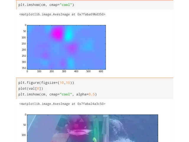
So I can say, let's create a function which takes our model's input as input and our fourth from last layer as output, that is that convolutional layer that I showed you. And then I'm going to take that and I'm going to pass into it the features of my first validation image and draw a picture of it for this picture, and here is my picture.

And so you can see it's done exactly what we thought it would do, which is it's had to figure out that there's a fishy bit here. So these fully convolutional networks have a nice side effect, which is that they allow us to find whereabouts the interesting parts are. The default parameters for max pooling are 2,2, so it's taking each 2x2 square and replacing it with the largest value in that 2x2 square.

So this is not the most high-res heat map we've ever seen. So the obvious thing to make it all more high-res would be to remove all the max pooling layers. So here's exactly the same thing as before, but I've removed all the max pooling layers. So that means that my model now remains at 22x40 all the way through, everything else is the same.

And that indeed does not give quite as accurate a result, we get 95.2 rather than 97.6. On the other hand, we do have a much higher resolution grid, so if we now do exactly the same thing to create the heat map, and the other thing we're going to do is resize the heat map to 360x640, and by default, this resize command will try and interpolate.

So it's going to replace big pixels with interpolated small pixels. And that gives us, for this image, this answer, which is much more interesting. And so now we can stick one on top of the other, like so. And this tells us a lot. It tells us that on the whole, this is doing a good job of saying the thing that mattered, the fishy thing, the albacore thing specifically, because we're asking here for the albacore plus.

Remember, the layer, that layer of the model is 8x22x40, so we have to ask how much like albacore is each of those areas, or how much like shark is each of those areas. So when we called this function, it returned basically a heat map for every type of fish, and so we can pass in 0 for albacore, or here's a cool one.

Class number 4 is nofish. So one of the classes you have to predict in this competition is nofish. So we could say, tell us how much each part of this picture looks like the nofish class. What happens is if you look at the nofish version, it's basically the exact opposite of this.

You get a big blue spot here, and pink or round it. The other thing I wanted to point out here is these areas of pinkishness that are not where the fish is. This is telling me that our model is not currently just looking for fish. It's also looking, if we look at this pink here, it's looking for particular characteristics of the boat.

So this is suggesting to me that since it's not all concentrated on the fish, I do think that there's some data leakage still coming through. I think we know everything about why it's working. We have set up a model where we've said we want you to predict each of the 8 fish classes.

We have set it up such that the last layer simply averages the answers from the previous layer. The previous layer we have set up so it has the 8 classes we need. So that's obviously the only way you can average and get the right number of classes. We know that SGD is a general optimization approach which will find a set of parameters which solves the problem that you give it and we've given it that problem.

So really, when you think of it that way, unless it failed to train, which it could for all kinds of reasons, unless it failed to train, it could only get a decent answer if it solved it in this way. If it actually looked at each area and figured out how fishy it is.

We're not doing attention models in this part of the course, per se. I would say for now, the simple attention model that I would do would be to find the largest area of the heat mat and crop that, and maybe compare that to the bounding boxes and make sure they look about the same and those that don't, you might want to hand fix.

And if you hand fix them, you have to give that back to the Kaggle community of course because that's hand labeling. And honestly, that's the state of the art. In terms of who wins the money in Kaggle, that's how the Kaggle winners have won these kinds of competitions is by having a two-stage pipeline where first of all they find the thing of interest and then they zoom into it and then they do a model on that thing.

Actually the other thing that you might want to do is to orient the fish so that the tail is kind of in the same place and the head is in the same place. Make it as easy as possible basically for your consonant to do what it needs to do.

You guys might have heard of another architecture called Inception. A combination of Inception plus ResNet won this year's ImageNet competition. And I want to give you a very quick hint as to how it works. I have built the world's tiniest little Inception network here in this screen. One of the reasons I want to show it to you is because it actually uses the same technique that we heard from Ben Bowles that he used.

Do you remember in his language model, Quid, Ben used a trick where he had multiple different convolution filter sizes and ran all of them and concatenated them together? That's actually what the Inception network does. To align the head and tail, the easiest way would be to hand annotate the head and hand annotate the tail.

That was what was done in the whale competition. Hand labeling always has errors, and indeed there are quite a few people in the forum who have various bounding boxes that they don't think are correct. It's great to have an automatic approach which ought to give about the same answer as the hand approach, and you can then compare the two and use the best of both worlds.

And in general, this idea of combining human intelligence and machine intelligence seems to be a great approach, particularly early on. You can do that for the first few bounding boxes to improve your bounding box model and then use that to gradually make the model have to ask you less and less for your input.

The heatmap you don't need to. The heatmap was just visualizing one of the layers of the network. We didn't use the bounding boxes, we didn't do anything special. It's just a side effect of this kind of model. You can visualize the last convolutional layer and in doing so we'll give you a heatmap.

There's so many ways of interpreting neural nets, and one of them is to draw pictures of the intermediate activations. You can also draw pictures of the intermediate gradients. There's all kinds of things you can draw pictures of. The Inception network is going to use this trick where we're going to use multiple different convolutional filter sizes.

Just like in ResNet, there's this idea of a ResNet block which is repeated again and again. In the Inception network, there's an Inception block which is repeated again and again. I've created a version of one here. I have one thing which takes my input and does a 1x1 convolution.

I've got one thing that takes the input and does a 5x5 convolution. I've got one thing that takes the input and does 2 3x3 convolutions. I've got one thing that takes the input and just average pulls it. And then we concatenate them all together. So what this is doing is each Inception block is basically able to look for things at various different scales and create a single feature map at the end which adds all those things together.

So once I've defined that, I can create a model that just goes Inception block, Inception block, Inception block, Comm2D, global average pulling 2D, output. I haven't managed to get this to work terribly well yet. I've got the same kind of results. I haven't actually tried submitting this to Kaggle.

Part of the purpose of this is to give you guys a sense of the kinds of things we'll be doing next year. This idea of we've built the basic pieces now of convolutions, fully connected layers, activation functions, SGD, and really from here, deep learning is putting these pieces together.

What are the ways people have learned about putting these things together in ways that solve problems as well as possible? And so the Inception network is one of these ways. And the other thing I wanted to do was to give you plenty of things to think about over the next couple of months and play with.

So hopefully this notebook is going to be full of things you can experiment with and maybe even try submitting some Kaggle results. I guess the warnings about the Inception network are a bit similar to the warnings about the ResNet network. Like ResNet, the Inception network is available, actually Keras.

I haven't converted one to my standard approach, but Keras has an Inception network that you can download and use. It hasn't been well-studied in terms of its transfer learning capabilities. Again I haven't seen people who have won Kaggle competitions using transfer learning of Inception network, so it's just a little bit less well-studied.

But like ResNet, the combination of Inception plus ResNet is the most recent image network. So if you are looking to really start with the most predictive model, this is where you would want to start. So I want to finish off on a very different note, which is looking at RNNs.

I've spent much more time on CNNs than RNNs. The reason is that this course is really all about being pragmatic. It's about teaching you the stuff that works, and in the vast majority of areas where I see people using deep learning to solve their problems, they're using CNNs. Having said that, some of the most challenging problems are now being solved with RNNs like speech recognition and language translation.

So when you use Google Translate now, you're using RNNs. My suspicion is you're going to come across these kinds of problems a lot less often, but I also suspect that in a business context, a very common kind of problem is a time series problem, like looking at the time series of click events on your website or e-commerce transactions or logistics or whatever.

These sequence-to-sequence RNNs we've been looking at, which we've been using to create Nietzschean philosophy, are identical to the ones you would use to analyze a sequence of e-commerce transactions and try to find anomalies. So I think CNNs are more practically important for most people in most organizations right now, but RNNs also have a lot of opportunities, and of course we'll also be looking at them when it comes to attentional models next year, which is figuring out in a really big image which part should we look at next.

Question - Does Inception have the merge characteristic? The Inception merge is a concat rather than that, which is the same as what we saw when we looked at Ben Bowles' quid NLP model. We're taking multiple convolution filter sizes and we're sticking them next to each other. So that feature basically contains information about 5x5 features and 3x3 features and 1x1 features.

And so when you add them together, you lose that information. ResNet does that for a very specific reason, which is we want to cause at all our residuals. In Inception, we don't want that. Inception, we want to keep them all in the feature space. The other reason I wanted to look at RNNs is that last week we looked at building an RNN nearly from scratch in Theano.

And I say nearly from scratch because there was one key step which it did for us, which was the gradients. Really understanding how the gradients are calculated is not something you would probably ever have to do by hand, but I think it can be very helpful to your intuition of training neural networks to be able to trace it through.

And so for that reason, this is kind of the one time in this course over this year and next year's course where we're going to really go through and actually calculate the gradients ourselves. So here is a recurrent neural network in pure Python. And the reason I'm doing a recurrent neural network in pure Python is this is kind of the hardest.

RNNs are the hardest thing to get your head around backpropagating gradients. So if you look at this and study this and step through this over the next couple of months, you will really be able to get a great understanding of what a neural net is really doing. There's going to be no magic or mystery because this whole thing is going to be every line of code, something that you can see and play with.

So if we're going to do it all ourselves, we have to write everything ourselves. So if we want a sigmoid function, we have to write the sigmoid function. Any time we write any function, we also have to create this derivative. So I'm going to use this approach where _d is the derivative function.

So I'm going to have relu and the derivative of relu. And I'll just kind of check myself as I go along that they look reasonable. The Euclidean distance and the derivative of the Euclidean distance. The cross entropy and the derivative of the cross entropy. And note here that I am clipping my predictions because if you have zeros or ones there, you're going to get infinities and it destroys everything.

So you have to be careful of this. This did actually happen. I didn't have this Euclidean at first and I was starting to get infinities and this is necessary. My softmax is the derivative of softmax. So then I basically go through and I double check that the answers I get with my versions are the same as the answers I get with the theana versions to make sure they're all correct and they all seem to be fine.

So I am going to use as my activation function relu, which means the derivative is relu derivative and my loss function is cross entropy derivative. I also have to write my own scan. So you guys remember scan. Scan is this thing where we go through a sequence one step at a time, calling a function on each element of the sequence.

And each time the function is going to get two things, it's going to get the next element of the sequence as well as the previous result of the call. So for example, scan of add two things together on the integers from 0 to 5 is going to give us the cumulative sum.

And remember the reason we do this is because GPUs don't know how to do loops, so our theano version used a scan. And I wanted to make this as close to the theano version as possible. In theano, scan is not implemented like this with a for loop. In theano, they use a very clever approach which basically creates a tree where it does a whole lot of the things kind of simultaneously and gradually combines them together.

Next year we may even look at how that works if anybody's interested. So in order to create our Nietzschean philosophy, we need an input and an output. So we have the eight character sequences, one hot encoded for our inputs, and the eight character sequences moved across by one, one hot encoded for our outputs.

And we've got our vocab size, which is 86 characters. So here's our input and output shapes, 75,000 phrases, each one has eight characters in, and each of those eight characters is a one-hot encoded vector of size 86. So we first of all need to do the forward pass. So the forward pass is to scan through all of the characters in the nth phrase, the input and output, calling some function.

And so here is the forward pass. And this is basically identical to what we saw in theano. In theano, we had to lay out the forward pass as well. So to create the hidden state, we have to take the dot product of x with its weight matrix and the dot product of the hidden with its weight matrix, and then we have to put all that through the activation function.

And then to create the predictions, we have to take the dot product of the hidden with its weight matrix and then put that through softmax. And so we have to make sure we keep track of all of the state that it needs, so at the end we will return the loss, the pre-hidden and pre-pred, because we're going to use them each time we go through.

In the back prop, we'll be using those. We need to know the hidden state, of course, we have to keep track of that because we're going to be using it the next time through the RNN. And of course, we're going to need our actual predictions. So that's the forward pass, very similar to the other one.

The backward pass is the bit I wanted to show you, and I want to show you how I think about it. This is how I think about it. All of my arrows, I've reversed their direction. And the reason for that is that when we create a derivative, we're really saying how does the input change, how does a change in the input impact the output?

And to do that, we have to use the chain rule, we have to go back from the end all the way back to the start. So this is our output last hidden layer activation matrix. This is our loss, which is adding together all of the losses of each of the characters.

If we want the derivative of the loss with respect to this hidden activation, we would have to take the derivative of the loss with respect to this output activation and multiply it by the derivative of this output activation with respect to this hidden activation. We have to then multiply them together because that's the chain rule.

The chain rule basically tells you to go from some function of some other function of x, the derivative is the product of those functions. So I find it really helpful to literally draw the arrows. So let's draw the arrow from the loss function to each of the outputs as well.

And so to calculate the derivatives, we basically have to go through and undo each of those steps. In order to figure out how that input would change that output, we have to basically undo it. We have to go back along the arrow in the opposite direction. So how do we get from the loss to the output?

So to do that, we need the derivative of the loss function. If we're going to go back to the activation function, we're going to need the derivative of the activation function as well. So you can see it here. This is a single backward pass. We grab one of our inputs, one of our outputs, and then we go backwards through each one, each of the 8 characters from the end to the start.

So grab our input character and our output character, and the first thing you want is the derivative of pre-pred. Remember pre-pred was the prediction prior to putting it through the softmax. So that was the bit I just showed you. It's the derivative of the softmax times the derivative of the loss.

So the derivative of the loss is going to get us from here back to here, and then derivative of the softmax gets us from here back to the other side of the activation function. That basically gets us to here. So that's what that gets us to. So we want to keep going further, which is we want to get back to the other side of the hidden.

We want to get all the way over now to here. For those of you that haven't done vector calculus, which I'm sure is many of you, just take my word for it. The derivative of a matrix multiplication is the multiplication with the transpose of that matrix. So in order to take the derivative of the pre-hidden times its weights, we simply take it by the transpose of its weights.

So this is the derivative of that part. And remember the hidden, we've actually got 2 arrows coming back out of it, and also we've got 2 arrows coming into it. So we're going to have to add together that derivative and that derivative. So here is the second part. So there it is with respect to the outputs, and there it is with respect to the hidden.

And then finally, we have to undo the activation function. So multiply it by the derivative of the activation function. So that's the chain rule that gets us all the way back to here. So now that we've got those two pieces of information, we can update our weights. So we can now say for the blue line, what are these weights now going to equal?

So we basically have to take the derivative that we got to at this point, which we called dprered. We have to multiply by our learning rate, which we're calling alpha. And then we have to undo the multiplication by the hidden state to get the derivative with respect to the weights.

And I created this little columnify function to do that. So it's turning a vector into a column, so essentially taking its transpose if you like. So that gives me my new output weights. My new hidden weights are basically the same thing. It's the learning rate times the derivative that we just calculated, and then we have to undo its weights and our new input weights, again at the learning rate, times the pre-hidden times the columnify version of x.

So I'll go through that very quickly. The details aren't important, but if you're interested it might be fun to look at it over the Christmas break or the next few days. Because you can see in this here is all of the steps necessary to do that through an RNN, which is also why we would never want to do this by hand again.

So when I wrote this code, luckily I did it before I got my code. You can see I've written after every one the dimensions of each matrix and vector because it just makes your head hurt. So thank God, Theano does this for us. But I think it's useful to see it.

So finally, I now just have to create my initial weight matrices, which are normally distributed matrices where these normal distribution, I'm going to use the square root of 2 divided by the number of inputs because that's that Glauro thing, ditto for my y matrix, and remember for my hidden matrix for a simple RNN, we will use the identity matrix to initialize it.

We haven't got to that bit yet, so it depends how we use this. At this stage all we've done is we've defined the matrices and we've defined the transitions. And whether we maintain state will depend entirely on what we do next, which is the loop. So here is our loop.

In our loop we're going to go through a bunch of examples, we should really go through all of them, but I was too lazy to wait. Run one forward step, and then one backward step, and then from time to time print out how we're getting along. So in this case, the forward step is passing to scan the initial state is a whole bunch of zeros.

So currently this is resetting the state, it's not doing it statefully. If you wanted to do it statefully, it would be pretty easy to change. You would have to have the final state returned by this and keep track of it and then feed it back the next time through the loop.

If you're interested, maybe you could try that. Having said that, you probably won't get great results because remember that when you do things statefully, you're much more likely to have gradients and activations explode unless you do a GIU or an LSTM. So my guess is it probably won't work very well.

So that was a very quick fly-through and really more showing you around the code so that if you're interested, you can check it out. What I really wanted to do was get onto this more interesting type of RNN, which is actually two interesting types of RNN called Long Short-Term Memory and Gated Recurrent Unit.

Many of you will have heard of the one on the left, LSTM. For stateful RNNs, you can't exactly have minivatches because you're doing one at a time. In our case, we were going through it in order. Using minivatches is a great way to parallelize things on the GPU and make things run faster, but we have to be careful about how you're thinking about state.

So LSTMs a lot of you will have heard about because they've been pretty popular over the last couple of years for all kinds of cool stuff that Google does. On the right, however, is the GRU, which is simpler and better than the LSTM. So I'm not going to talk about the LSTM, I'm going to talk about the GRU.

They're both techniques for building your recurrent neural network where your gradients are much less likely to explode. They're another great interesting example of a clever architecture, but it's just going to be more of using the same ideas that we've seen again and again. What we have here on the right-hand side is this box.

It's basically zooming into what's going on inside one of these circles in a GRU. So normally in our standard RNN, what's going on in here is pretty simple, which is we do a multiplication by this WH weight matrix and stick it through an activation function, and we grab our input, do it by a multiplication by weight matrix and grab its, and do it through its activation function, and we add the two together.

At GRU, though, it's going to do something more complex. We still have the input coming in and the output going out, so that's what these arrows are. They're representing our new input character and our prediction. But what's going on in the middle is more complex. We still have our hidden state, just like before.

But in a normal RNN, the hidden state each time simply updates itself. It just goes through a weight matrix and an activation function and updates itself. But in this case, you can see that the loop looks like it's going back to come direct with self, but then there's this gate here.

So it's actually not just a self-loop, there's something more complicated. So in order to understand what's going on, we're going to have to follow across to the right hand side. So on the right hand side, you can see that the hidden state is going to go through another gate.

So what's a gate? A gate is simply a little mini-neural network which is going to output a bunch of numbers between 0 and 1, which we're going to multiply by its input. In this particular one, the R stands for reset. And so the numbers between 0 and 1, if they were all 0, then the thing coming out of the reset gate would be just a big bunch of 0's.

In other words, it would allow this network to forget the hidden state. Or it could be a big bunch of 1's which would allow the network to remember all of the hidden state. Do we want it to remember or forget? We don't know, which is why we implement this gate using a little neural network.

And this little neural network is going to have two inputs, which is the input to the gate, the input to the GIU unit, and the current hidden state. And so it's going to learn a set of weights that it's going to use to decide when to forget. So it's now got the ability to forget what it knows.

And that's what the reset gate does. So assuming that the reset gate has at least some non-zero entries, which it most surely will most of the time, then whatever comes through we're going to call h_tilde, or in my code I call it h_new. So this is the new value of the hidden state after being reset.

And so then finally, that goes up to this top bit here. The original hidden state goes up to this top bit here. And then there's a gate which decides how much of each one should we have. So this is an update gate. This update gate is going to decide if it's 1, we'll take more from this side.

If it's 0, we'll take more from this side. And again, that's implemented as a little neural network. I think the easiest way to understand this is probably to look at the code. So I have implemented this in Theano. You can use a GIU in Keras by simply replacing the words simple RNN with GIU.

So you don't really need to know this to use it, and you get pretty good results. But here's what it looks like when implemented. We don't just have a hidden input weight matrix and an output weight matrix anymore, we also have a hidden input weight matrix for our little reset gate, and for our update gate.

So here is the definition of a gate. A gate is something which takes its inputs, its hidden state, its hidden state weights, its input weights, and its biases. It does a dot product of the x with w_x, a dot product of h with w_h, and adds the biases and sticks to its true or single action.

So that's what I meant by a mini-neuronet. It's hardly a neuronet, it's just got one layer. So that's the definition of the reset gate and the update gate. And so in our step function, this is the thing that runs each time on the scan, it looks exactly the same as what we looked at last week.

The output equals the hidden state times the hidden weight matrix plus the hidden biases. The new hidden state equals our inputs times its weights and the hidden state times its weights plus the biases, but this time the hidden weights are multiplied by the reset gate. And the reset gate is just a little neural net.

So now that we have h new, our actual new hidden state is equal to that times 1 minus the update gate plus our previous hidden state times the update gate. So you can see that update plus 1 minus update will add to 1. So you can see why it's been drawn like so, which is that this can really be anywhere at either end or somewhere in between.

So the update gate decides how much is h new going to replace the new hidden state with. So actually, although people tend to talk about LSTMs and GRUs as being pretty complex, it really wasn't that hard to write. The key outcome of this though is that because we now have these reset and update gates, is that it has the ability to learn these special sets of weights to make sure that it throws away state when that's a good idea, or to ignore state when that's a good idea.

And so these extra degrees of freedom allow SGD to find better answers, basically. And so again, this is one of these things where we're coming up with architectures which just try to make it easier for the optimizer to come up with good answers. Everything after this is identical to what we looked at last week.

That goes into the scan function, to calculate the loss, we calculate the gradients, we do the SGD updates, and we chuck it into the scan function. So I think really the main reason I wanted to do all that today was to show you the backdrop example. I know some learning styles are more detail oriented as well, and so I think some of you hopefully will have found that helpful.

Any time you find yourself wondering how the hell did this neural network do this, you can come back to this piece of code and that's all it did. That's all that's going on. That's one way of thinking about it. Where you really get successful with neural nets though is when you go to a whole other level and you don't think of it at that level anymore, but instead you start thinking, if I'm an optimizer and I'm given an architecture like this, what would I have to do in order to optimize it?

And once you start thinking like that, then you can start thinking in this kind of like upside down way that is necessary to come up with good architectures. You can start to understand why it is that this convolution layer followed by this average pooling layer gives the answers that it does.

Why does it work? You get that real intuition for what's going to work for your problem. So there's two ways, two levels at which you need to think about neural nets. The sooner you can think of it at this super high level, I feel like the sooner you'll do well with them.

One of the best ways to do that is to, over the next couple of weeks, run this FISH notebook yourself and screw around with it a lot. Make sure that you know how to do these things that I did where I actually create a little function that allows me to spit out the output of any of the layers and visualize it.

Make sure you kind of know how to inspect it and really look at the inputs and outputs. I think that's the best way to get an intuition. So this was kind of like, particularly the first half of this class was a bit of a preview of next year. In the first 6 weeks, you learn all the pieces.

And then today, we very rapidly tried putting those pieces together in a thousand different ways and saw what happened. There's a million more ways that we know of, and probably a billion more ways we don't know of. So knowing this little set of tools, convolutions, fully connected layers, activation functions, SGD, you're now able to be an architect, create these architectures.

Keras' functional API makes it ridiculously easy. I created all of the architectures you see today, this week, while I was sick and my baby wasn't sleeping. My brain was not even working, that's how easy Keras makes this. It takes a few weeks to build your comfort level up, but hopefully you can try that.

And most importantly, over the next few weeks, as Rachel and I, maybe with some of your help, start to develop the MOOC, you guys can stay talking on the forums about keep working through whatever problems you're interested in. Whether it be the projects that you want to apply these things to in your own organizations or your personal passion projects or if you want to try and win a competition or two.

Rachel and I are still going to be on the forums. And then in a few weeks time, when the MOOC goes online, hopefully there's going to be thousands of people joining this community. So we'll be like the seed. So I really hope you guys will stay a part of it and help.

Can you imagine that first day when half the people still think that a python is a snake and don't know how to connect to an AWS instance? You'll all be able to say, read the wiki, here's the page, oh yeah, I had that problem too. And hopefully our goal here is to create a new generation of deep learning practitioners, people who have useful problems that they're trying to solve and can use this tool to solve them, rather than create more and more exclusive, heavily mathematical content that's designed to put people off.

So that's our hope. That's really why we're doing this. Rachel, anything else that we should add before we wrap up? Okay, well thank you so much. It really has been a genuine pleasure and I'm so happy to hear that most of you are going to see you again next year.

You guys obviously will get first dibs on places for next year's course. If the MOOC successful, next year's course could be quite popular, so I do suggest that you do nonetheless get your applications in not too late. They'll certainly go through with priority. Be aware if you're not already, we don't send email much, really the forums is our main way to communicate and Slack to some extent.

So if you want to see what's going on, that's the places to look. And of course, our wiki is the knowledge base that we're creating for everybody. So anytime you see something missing on the wiki or something you think could be improved, edit it. Even if you're not sure if you're saying the right thing, you can add a little comment after it's saying "I'm not sure if this is correct." The next person coming along will help you.

Thanks so much everybody. I hope you all have a great vacation season.