Hi and welcome to lesson 20. In the last lesson we were about to learn about implementing mixed precision training. Let's dive into it. And I'm going to fiddle with other things just because I want to really experiment. I just love fiddling around. So one thing I wanted to do is I wanted to get rid of the DDPMCB entirely.

We made it pretty small here, but I wanted to remove it. So much as Janice said, isn't it great the callbacks make everything so cool. I wanted to show we can actually make things so cool without callbacks at all. And so to do that, I realized what we could do is we could put noisify inside a collation function.

So the collation function, if you remember back to our datasets notebook, which was going back to notebook five and you've probably forgotten that by now. So go and reread that to remind yourself. It's the function that runs to take all of the, you know, you've basically each kind of row of data.

It will be a separate tuple, but then it hits the collation function and the collation function turns that into tensors. You know, one tensor representing the independent variable, one tensor representing the dependent variable, something like that. And the default collation function is called, not surprisingly, default collate. So if our collation function calls that on our batch and then grabs the X part, which is it's always been the same for the last few things.

That's the image because we use because datasets uses dictionaries. So we're going to grab the image. Then we can call noisify on that collated batch. Then that's exactly the same thing as Tunis before batch did because before batch is operating on the thing that came out of the default collect function.

So we could just do it in a click function. So if we do it here and then we create a DDPM data loader function, which just creates a data loader from some dataset that we pass in with some batch size with that collation function. Then we can create our DL's not using data loaders from data loaders from DD.

But instead of that, the original, you know, the plane in it that we created for data loaders. And again, you should go back and remind yourself of this. You just pass in the data loaders for training and test. So there's our two data loaders. So with that, we don't need a DDPM callback anymore.

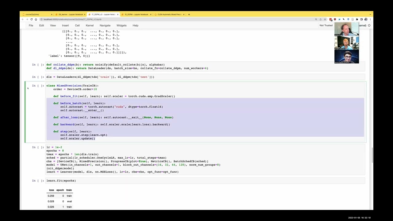
All right. So now that we've, you know, and again, this is this is not required for mixed precision. This is just because I wanted to experiment and flex our muscles a little bit of trying things out. So here's our mixed precision callback. And this is a training callback. And basically, if you Google for PyTorch mixed precision, you'll see that the docs show the typical mixed precision basically says with autocast, device equals CUDA, type equals float 16, get your predictions and core your loss.

So, again, remind yourself if you've forgotten that this is called a context manager and context managers when they start call something called done to enter. And when they finish, they call something called done to exit. So we could therefore put the torch autocast into an attribute and call done to enter before the batch begins.

And then after we've calculated the loss, we want to finish that context manager. So after loss, we call autocast done to exit. And so I had to add this. So you'll find now in the 09 learner that there's a section called updated version since the lesson where I've added an after predict, an after loss, an after backward and an after step.

And that means that a callback can now insert code at any point of the training loop. And so we haven't used all of those different things here, but we certainly do want. Yeah, after loss, it better do that. And then, yeah, this is just code that has to be run according to it, to the PyTorch docs.

So instead of calling lost dot backwards, you have to call scalar dot scale, lost dot backward. So we replace our backward in the train callback with something called scalar dot scale, lost dot backward. And then it says that finally, when you do the step, you don't call optimizer dot step, you call scalar dot step optimizer scalar dot update.

So we've replaced step with scalar dot step scalar dot update. So that does all of the things in here. And the nice thing is now that this exists, we don't have to think about any of that. We can add mixed precision to anything, which is really nice. And so we now, as you'll see, CB is no longer has a DDPM CB, but we do have the mixed precision.

And that's a train callback. So we just need a normal learner, not a train learner. And we initialize our DDPM. Now, to get benefit from mixed precision, you need to do quite a bit at a time. You know, your GPU needs to be busy. And on something as small as fashion MNIST, it's not easy to keep a GPU busy.

So that's why I've increased the batch size by four times. Now, that means that each epoch, it's going to have four times less batches because they're bigger. That means it's got four times less opportunities to update. And that's going to be a problem because if I want to have as good a result as to niche CAD and as I had here in less time, that's the whole purpose of this is to do it in less time, then I'm going to need to, you know, increase the learning rate and maybe also increase the epoch.

So I increase the epochs up to eight from five and I increase the learning rate up to one in egg two. And yeah, I've found I could train it fine with that once I use the proper initialization and most importantly, use the optimization function that has epsilon of one in egg five.

And so this trains, even though it's doing more epochs, this trains about twice as fast. And gets the same result. Does that make sense so far? Yeah, it was great. Cool. Now, the good news is actually we don't even need to write all this because there's a nice library from Hugging Face, originally created by Silver, who used to work with me at FastAI and went to Hugging Face and kept on doing awesome work.

And he started this project called Accelerator, which he now works on with another FastAI alum named Zach Riele, and accelerates a library that provides this in-court accelerator that does things to accelerate your training loops. And one of the things it does is mix precision training and it basically handles these things for you.

It also lets you train on multiple GPUs. It also lets you train on TPUs. So by adding a train_cb subclass that will allow us to use Accelerate, that means we can now hopefully use TPUs and multi-GPU training and all that kind of thing. So the Accelerate docs show that what you have to do to use Accelerate is to create an accelerator, tell it what kind of mixed precision you want to use.

So we're going to use 16-bit floating point FP16. And then you have to basically call Accelerator.Prepare and you pass in your model, your optimizer, and your training and validation data loaders. And it returns you back a model, an optimizer, and training and validation data loaders, but they've been wrapped up in Accelerate.

And Accelerate is going to now do all the things we saw you have to do automatically. And that's why that's almost all the code we need. The only other thing we need is we didn't tell it how to change our loss function to use Accelerate, so we actually have to change backward.

That's why we inherit from train_cb. We have to change backward to not call loss.backward, but self.accelerate.backward and pass in loss. OK. And then I had another idea of something I wanted to do, which is I like the idea that Noisify, I've copied Noisify here, but rather than returning a tuple of tuples, I just return a tuple with three things.

I think this is neater to me. I would like to just have three things in the tuple. I don't want to have to modify my model. I don't want to have to modify my training callback. I don't want to do anything tricky. I don't even want to have a custom collation function.

Sorry, I want to have a custom collation function, but I don't want to have a modified model. So I'm going to go back to using a UNet2D model. So how can we use a UNet2D model when we've now got three things? And what I did in my modified ladder, just underneath it, sorry, actually what I did is I modified train_cb to add one parameter, which is number of inputs.

And so this tells you how many inputs are there to the model. Normally you would expect one input, but our model has two inputs. So here we say, okay, so accelerate_cb is a train_cb. So when we call it, we say we're going to have two inputs. And so what that's going to do is it's just going to remember how many you asked for.

And so when you call predict, it's not going to pass learn.batch0. It's going to call star learn.batch colon self.name_inputs. And ditto, when you call the loss function, it's going to be the rest. So it's star learn.batch self.add_imp onwards. So this way you can have one, two, three, four, five inputs, one, two, three, four, five outputs, whatever you like.

And it's just up to you then to make sure that your model and your loss function take the number of parameters. So the loss function is going to first of all take your creds and then, yeah, however many non-inputs you have. So that way, yeah, we now don't need to replace anything except that we did need to do the thing to make sure that we get the dot sample out.

So I just had a little, this is the whole DDPMCB callback now, DDPMCB2. So after the predictions are done, replace them with the dot sample. Right. So that's nice and easy, you know. So we end up with quite a bit of pieces, but they're all very decoupled, you know.

So with mini AI, you know, with and with AccelerateCB and whatever, I guess we should export these actually into a nice module. Well, if you had all those, then, yeah, you wouldn't have AccelerateCB. The only thing you would need would be the noisify and the collation function and this tiny callback.

And then, yeah, use our learner and fit and we get the same result as usual. And this takes basically an identical amount of time because at this point I'm not using all the GPU or TPU or whatever. I'm just using mixed precision. So this is just a shortcut for this.

It's not a huge shortcut. The main purpose of it really is to allow us to use other types of accelerators or multiple accelerators or whatever. So we'll look at those later. Does that make sense so far? Yeah. Yeah. Accelerator is really powerful and pretty amazing. Yeah, it is. And I know like a lot of, yeah, like I know Kat Carlson uses it in all her K diffusion code, for example.

Yeah, it's used a lot out there in the real world. Yeah. I've got one more thing I just want to mention briefly. Just a sneaky trick. I haven't even bothered training anything with it because it's just a sneaky trick. But sometimes thinking about speed, loading the data is the slow bit.

And so particularly if you use Kaggle, for example, on Kaggle, you get two GPUs, which is amazing, but trying to get two CPUs, which is crazy. So it's really hard to take advantage of them because the amount of time it takes to open a PNG or a JPEG, your GPU is sitting there waiting for you.

So if your data loading and transformation process is slow and it's difficult to keep your GPUs busy, there's a trick you can do, which is you could create a new data loader class, which wraps your existing data loader and it replaces DunderIdder. Now, DunderIdder is the thing that gets called when you use a for loop, right?

Or when you use NextIdder, it calls this. And when you call this, you just go through the data loader as per usual. So that's what DunderIdder would normally do. But then you also go through I from zero to by default two and then you spit out the batch. And what this is going to do is it's going to go through the data loader and spit out the batch twice.

Why is that interesting? Because it means every epoch is going to be twice as long, but it's going to only load and augment the data as often as one epoch, but it's going to give you two epochs worth of updates. And basically, there's no reason to have a whole new batch every time.

You know, looking at the same batch two or three or four times at a row is totally fine. And what happens in practice is you look at that batch, you do an update, get 20 part of the weight space, look at exactly the same batch and find out now where to go in the in the weight space.

It's still, yeah, basically equally useful. So I just wanted to add this little sneaky trick here, particularly because if we start doing more stuff on Kaggle, we'll probably want to surprise all the Kagglers with how fast our mini AI solutions are. And they'll be like, how is that possible?

We'll be like, oh, we're using our, you know, two GPUs, six to accelerate. Thinking about how do we use the two GPUs and like, oh, and we're, you know, using, you know, getting out, loading, flying through using multi L. I think that'd be pretty sweet. So that's that. Nice.

Yeah, it's great to see the various different ways that we can use mini AI to do to do the same thing, I guess, or, you know, however you feel like doing it or whatever works best for you. Yeah. And I'll be curious to see if other people find other ways to, you know, I'm sure there's so many different ways to to handle this problem.

I think it's an interesting, interesting problem to solve. And I think for the homework, it'd be useful for people to run some of their own experiments, maybe either use these techniques on other data sets or see if you can come up with other variants of these approaches or come up with some different noise schedules to try.

It would all be useful. Any other thoughts of exercises people could try? Yeah, I mean, getting away with less than a thousand steps. Yeah, a thousand steps happening in the final 200. So why not just train with only 200 steps? Yeah, that steps would be good. Yeah, because the sampling is actually pretty slow.

So that's a good point. Yeah, yeah, I was gonna say something similar in terms of like, yeah, many, I guess, work with less number of steps. You know, you have to adjust the noise schedule appropriately and you have to, I guess there's maybe a little bit more thought into some of these things.

Or, you know, another aspect is like, when you're selecting the time step during training, right now we select it randomly, kind of uniformly, each time step has equal probability of being selected. Maybe different probabilities are better and some papers do analyze that more carefully. So that's another thing to play around with as well.

That's almost kind of like, I guess there are almost two ways of doing the same thing in a sense, right? If you change that mapping from t to beta, then you could reduce t and have different betas would kind of give you a similar result as changing the probabilities of the t's, I think.

Yeah, I think there's definitely, they're kind of similar, but potentially something complementary happening there as well. And I think those could be some interesting experiments to study that and also the sort of noise levels that you do choose affect the sort of behavior of the sampling process. And of course, what features you focus on.

And so maybe as people play around with that, maybe they'll start to notice how using different noise levels or different noise schedules affect maybe some of the features that you see in the final image. And that could be something very interesting to study as well. Right. Well, let me also say it's been really fun doing something a bit different, which is doing a lesson with you guys rather than all on my lonesome.

I hope we can do this again because I've really enjoyed it. Yeah, it was great. So, of course, now we're, you know, strictly speaking in the recording, we'll next up see Johnno, who's actually already recorded his thanks to the Zoom mess up, but stick around. So I've already seen it.

Johnno's thing is amazing. So you definitely don't want to miss that. Hello, everyone. So today, depending on the order that this ends up happening, you've probably seen Denise a DDPM implementation where we're taking the default training call back and doing some more interesting things with preparing the data for the learner or interpreting the results.

So in these two notebooks that I'm going to show, we're going to be doing something similar, just exploring like what else can we do besides just the classic kind of classification model or where we have some inputs and a label. And what else can we do with this mini AI setup that we have.

And so in the first one, we're going to approach a kind of classic AI art approach called style transfer. And so the idea here is that we're going to want to somehow create an artistic combination of two images where we have the structure and layout of one image and the style of another.

So we'll look at how we do that. And then we'll also talk along the way in terms of like, why is this actually useful beyond just making pretty pictures. So to start with, I've got a couple of URLs for images. You're welcome to go and slip in your own as well and definitely recommend trying this notebook with some different ones just to see what effects you can get.

And we're going to download the image and load it up as a tensor. So we have here a three channel image 256 by 256 pixels. And so this is the kind of base image that we're going to start working with. So before we talk about styles or anything, let's just think what is our goal here.

We'd like to do some sort of training or optimization. We'd like to get to a point where we can match some aspect of this image. And so maybe a good place to start is to just try and do what can we start from a random image and optimize it until it matches pixel for pixel exactly.

And that's going to help us get this. Yeah. I think that might be helpful is if you type style transfer deep learning into Google images, you could maybe show some examples so that people will see what their goal is. Yeah, that's a very good point. So let's see. This is a good one here.

We've got the Mona Lisa as our our base. But we've managed to apply some how some different artistic styles to that same base structure. So we have the Great Wave by Psaki. We have Starry Night by Vincent Mango. This is some sort of Kandinsky or something. Yeah. So this is our end goal to be able to take the overall structure and layout of one image and the style from some different reference image.

And in fact, this was the first ever I think fast AI generative modeling lesson looked at style transfer. It's it's been around for a few years. It's kind of a classic technique. And it's really I think a lot of the students when we first did it found it extremely useful way of better understanding, like, you know, flexing their deep learning muscles, understanding what's going on.

And also created some really interesting new approaches. So hopefully we'll see the same thing again. Maybe some students will be able to show some really interesting results from this. Yeah. And I mean, today we're going to focus on kind of the classic approach. But I know one of the previous students from fast AI did a whole different way of doing that style loss that we'll maybe post in the forums or, you know, I've got some comparisons that we can look at.

So, yeah, definitely a fruitful field still. And I think after the initial hype of like everyone was excited about style transfer apps and things five years ago. I feel like there's still some things to explore there. Very creative and fun little and divergent in the deep learning world. OK, so our first step in getting to that point is being able to optimize an image.

And so up until now, we've been optimizing like the weights of a neural network. But now you want to go to something a bit more simple and we just want to optimize the raw pixels of an image. Do you mind if you scroll up a bit to the previous code just so we can have a look at it?

So there's a couple of interesting points about this code here is, you know, we're not we're not cheating. Well, not really. So we're so yeah, we've seen how to download things in the network before. So we're using fastcodes URL read because we're allowed to. And then I think we decided we weren't going to write our own JPEG parser.

So TorchVision actually has a pretty good one, which a lot of people don't realize exists. And a lot of people tend to use PIL, but actually TorchVision has a more performant option. And it's actually quite difficult to find any examples of how to use it like this. Here's some code you can borrow.

Yeah, actually, Google load image from a URL in PyTorch. All of the examples are going to use PIL. And that's what I've done historically is use the requests library to download the URL and then feed that into PIL's image.open function. So yeah, that was fun when I was working with Jeremy on this notebook.

Like that's how I was doing it. It's with me breaking the rules. And let's see if we can do this directly into a tensor without this intermediate step of loading it with with pillow. Cool. Okay. So how are we going to do this image optimization? Well, first thing is we don't really have a data set of lots of training examples.

We just have a single target and a single thing we're optimizing. And so we built this linked data set here, which is just going to follow the PyTorch data set standard. We're going to tell it how to get a particular item and what our length is. But in this case, we're just always going to return zero zero.

We're not actually going to care about the results from this data set. We just want something that we can pass to the learner to do some number of training iterations. So we create like a thick dummy data set with a hundred items and then we create our data loaders from that.

And that's going to give us a way to train for some number of steps without really caring about what this data is. So does that make sense? Yeah. So just to clarify the reason we're doing this. So basically, the idea is we're going to start with that photo you downloaded and I guess you're going to be downloading another photo.

So that photo is going to be like the content. We're going to try to make it continue to look like that lady. And then we're going to try to change the style so that the style looks like the style of some other picture. And the way we're going to be doing that is by doing an optimization loop with like SGD or whatever.

So the idea is that each step of that, we're going to be moving the style somehow of the image closer and closer to one of those images you downloaded. So it's not that we're going to be looping through lots of different images, but we're just going to be looping through steps of a optimization loop.

Is that the idea? Exactly. And so, yeah, we can create this data loader. And then in terms of the actual model that we're optimizing and passing to the learner, we created this tensor model class, which just has whatever tensor we pass in as its parameter. So there's no actual neural network necessarily.

We're just going to pass in a random image or some image-shaped thing, a set of numbers that we can then optimize. So just in case people have forgotten that, so to remind people, when you put something in an n-end or parameter, it doesn't change it in any way. It's just a normal tensor, but it's stored inside the module as being something as being a tensor to optimize.

So what you're doing here, Jono, I guess, is to say I'm not actually optimizing a model at all. I'm optimizing an image, the pixels of an image directly. Exactly. And because it's in a parameter, if we look at our model, we can see that, for example, model.t, it does require grad, right?

Because that's already set up, because this n-end module is going to look for any parameters. And if our optimizer is looking at, let's look at the shape of the parameters. So this is the shape of the parameters that we're optimizing. This is just that tensor that we passed in, the same shape as our image.

And this is what's going to be optimized if we pass this into any sort of learner fit method. OK, so this model does have a thing being passed to forward, which is x, which we're ignoring. And I guess that's just because our learner passes something in. So we're making life a bit easier for ourselves by making the model look the way our learner expects.

Yeah. And we could do that using like train_cb or something if we wanted to. But this seems like a nice, nice, easy way to do it. Yeah, so I mean, this is the way I've done it. If you do want to use train_cb, you can set it up with a custom predict method that is just going to call the model forward method with no parameters.

And if you want, likewise, just calling the loss function on just the predictions. But if you want to skip this because we take this argument x equals zero and never use it, that should also work without this callback. So either way is fine. This is a nice approach if you have something that you're using an existing model, which expects some number of parameters or something.

Yeah, you can just modify that training callback, but we almost don't need to in this case. OK, so let's see. Let's put this in a learner. Let's optimize it with some loss function. Oh, just to clarify, I get it. So the get_loss you had to change because normally we pass a target to the loss function.

Yes, it's learner.prids and then learner.batch. And again, we could avoid, we could remove that as well if we wanted to by having our loss function take a target that we then ignore. Yeah, exactly. So both other approaches, I like this because we're going to kind of be building on this idea of modifying the training callback in the DDPM example and the other examples.

But in this case, it's just these two lines change. This is how we get our model predictions. We just call the forward method, which returns this image that we're optimizing. And we're going to evaluate this according to some loss function that just takes in an image. So for our first loss function, we're just going to use the mean squared error between the image that we are generating, like this output of our model and that content image that's our target.

Right. So we're going to set up our model, start it out with a random image like this above. We're going to create a learner with a dummy data loader for 100 steps. Our loss function is going to be this mean squared error loss function, set a learning rate and an optimizer function.

The default would probably also work. And if we run this, something's going to happen. Our loss is going to go from a non-zero number to close this error. And we can look at the final result, like if we call learn.model and show that as an image versus the actual image, we'll see that they look pretty much identical.

So just to clarify, this is like a pointless example, but what we did, we started with that noisy image she showed above. And then we used SGD to make those pixels get closer and closer to the lady in the sunglasses. Not for any particular purpose, but just to show that we can turn noisy pixels into something else by having it follow a loss function.

Make the pixels look as much as possible, like that idea in the sunglasses. Exactly. And so in this case, it's a very simple loss. There's like a one direction that you update, so it's almost trivial to solve, but it still helps us get the framework in place. But just seeing this final result is not very instructive because you almost think, well, did I get a bug in my code?

Did I just duplicate the image? How do I know this is actually doing what we expect? And so before we even move on to any more complicated loss functions, I thought it was important to have some sort of more obvious way of doing progress. So I've created a little logging callback here that is just after every batch, it's going to store the output as an image.

I guess after every 10 batches here by default. Oh, yes. Yeah. Sorry. So we can set how often it's going to update and then every 10 iterations or 50 iterations, whatever we set the log every argument to, it's going to store that in a list. And then after the training is done, after that, we're just going to show those images.

And so everything else the same as before, but passing in this extra logging callback, it's going to give us the kind of progress. And so now you can see, OK, there is actually something happening. We're starting from this noise after a few iterations. Already, most of it is gone.

And by the end of this process, it looks exactly like the content image. So I really like this because what you've basically done here is you've now already got all the pooling and infrastructure in place you need to basically create a really wide variety of interesting outputs that could either be artistic or like, you know, there could be more like image reconstruction, super resolution, colorization, whatever.

And you just have to modify the loss function. And I really like the way you've created the absolute easiest possible first and fully checked it. And before you start doing the fancy stuff and now you kind of, I guess, feel really comfortable doing the fancy stuff because you know that's all in place.

Yeah, exactly. And we know that we're going to see some tracking. Hopefully it'll be visually obvious if things are going wrong and we know exactly what we need to modify. If we can now express some desired property that's more interesting than just like mean squared error to a target image, then we could have everything in place to optimize.

And so this is now really fun to like, OK, let's think about what other loss functions we could do. Maybe we wanted to match an image, but also have a particular overall color. Maybe we want some some more complicated thing. And so towards that, like towards starting to get a more richer like measure of what this output image looks like, we're going to talk about extracting features from a pre-trained network.

And this is kind of like the core idea of this notebook is that we have these big convolutional neural networks. This one is a much older architecture. And it's a relatively simple compared to some of the big, you know, dense nets and so on used today. It's actually a model like our Pre-ResNet Fashioned MNIST model.

It's basically almost the same as VGG16. Yeah, yeah, exactly. And so we're feeding in an image and then we have these like convolutional layers, downsampling, convolution, you know, downsampling with max pooling up until some final prediction. Oh, but can I just point something out? There's one big difference here, which is that seven by seven by five twelve, if you can point at that.

Normally nowadays and in our models, we tried, you know, using an adaptive or global pooling to get down to a one by one by five twelve. VGG16 does something which is very unusual by today's standards, which is it just flattens that out into a one by one by four or nine six.

Which actually might be a really interesting feature of VGG. And I've always felt like people might want to consider training, you know, res nets and stuff without the global pooling and instead do the flattening. The reason we don't do the flattening nowadays is that that very last linear layer that goes from one by one by four or nine six to one by one by a thousand, because this is an image net model, is going to need an awfully big weight matrix.

You've got a four or nine six by a thousand weight matrix as a result of which this is actually horrifically memory intensive for a reasonably poor performing model by modern standards. But yeah, I think that doing that actually also has some some benefits potentially as well. Yeah. And in this case, we are not even really interested in the classification side.

We're more excited about the capacity of this to extract different features. And so the idea here and maybe I should pull up this classic article looking at like what do neural networks learn and trying to visualize some of these features. And this is something we've mentioned before with these big pre-trained networks is that the early layers tend to pick up on very simple features, edges and shapes and textures and those get mixed together into more complicated textures.

And by the way, this is just trying to visualize like what what kind of input maximally activates a particular like output on each of these layers. And so it's a great way to see like what kinds of things that's learning. And so you can see as we move deeper and deeper into the into the network, we're getting more and more complicated, like hierarchical features.

And so we've looked at the Zeiler and Fergus paper before that which is an earlier version doing something like this to see what kind of features were available. So we'll link to this distill paper from the forum and the course lesson page because it's actually a more modern and fancy version kind of the same thing.

Yeah. Also note the names here. All of these people are worth following. Chris does amazing work on interpretability and Alexander Modvinsov we'll see in the second notebook that I look at today and doing all sorts of other cool stuff as well. And anyway, so we want to think about like let's extract the outputs of these layers in the hope that they give us a representation of our image that's richer than just the raw pixels.

So we can list the idea being there that if we had another if we were able to change our image to have the same features at those various types that you were just showing us that then it would like have similar textures or similar kind of higher level concepts or whatever.

Exactly. So if you think of this like 14 by 14 feature map over here, maybe it's capturing that there's an eye in the top left and some hair on the top right, these kind of abstract things. And if you change the brightness of the image, it's unlikely that it's going to change what features are stored there because the networks learned to be somewhat invariant to these like rough transformations, a bit of noise, a bit of changing texture early on.

It's not going to affect the fact that it still thinks this looks like a dog and a few layers before that, that it still thinks that part looks like a nose and that part looks like an ear. Maybe the more interesting bits then for what you're doing are those earlier layers where it's going to be like there's a whole bunch of kind of diagonal lines here or there's a kind of a loopy bit here because then if you replicate those, you're going to get similar textures without changing the semantics.

Exactly. Yeah. So, I mean, I guess let's load the model and look at what the layers are. And then in the next section, we can try and like see what kinds of images work when we optimize towards different layers in there. And so this is the network we have, revolutions, relu, max pooling, all of this we should be familiar with by now.

And it's all just in one big and in dot sequential. This doesn't have the head. So we said dot features. If you did this without you'd have then the this is like the features sub sub sub network. That's everything up until some point. And then you have the flattening and the classification, which we are kind of just throwing away.

So this is the body of the network. And we're going to try and tag into various layers here and extract the outputs. But before we do that, there's one more bit of admin we need to handle. And this was trained on a normalized version of ImageNet, right, where you took the data set me and the data set standard deviation and use that to normalize your images.

So if we want to match what the data looked like during training, we need to match that normalization step. And we've done this on grayscale images where we just subtract the mean divide by the standard deviation. But with three channel images, these RGB images, we can't get away with just saying, let's subtract our mean from our image and divide by the standard deviation.

You're going to get an error that's going to pop up. And this is because we now need to think about broadcasting and these shapes a little bit more carefully than we can with just a scalar value. So if we look at the mean here, we just have three values, right, one for each channel, the red, green and blue channels, whereas our content image has three channels and then 256 by 256 for the spatial dimensions.

So if we try and say content image divided by the mean or minus the mean, it's going to go from right to left and find the first non-unit axis. So anything with a size greater than one. And it's going to try and line those up. And in this case, the three and the 256, those aren't going to match.

And so we're going to get an error. More perniciously, if the shape did happen to match, that might still not be what you intended. So what we'd like is to have these three channels map to the three channels of our image and then somehow expand those values out across the two other dimensions.

And the way we do that is we just add two additional dimensions on the right for our image.net.mean. And you could also do the unsqueezed minus one, the unsqueezed minus one. But this is the kind of syntax that we're using in this course. And now our shapes are going to match because we're going to go from right to left if it's a unit dimension size one, we're going to expand it out to match the other tensor.

And if it's a non-unit dimension, then the shapes have to match. And that looks like it's the case. And so now with this reshaping operation, we can write a little normalized function, which we can then apply to our content image. And I'm just checking the min and the max to make sure that this roughly makes sense.

And we could check the mean as well to make sure that the mean is somewhat close to zero. OK, in this case, less maybe because it's a darker image than average, but at least we are doing the operation. It seems like the math is correct. And now the sharing the channel wise mean would be interesting.

Oh, yes. So that would be the mean over the dimensions. One and two, I think. I think you have to type all one comma to this. I wasn't sure which way around. Yeah, I always forget to say. OK, so our blue channel is brighter than the others. And if you go back and look at our image, maybe believe that the image interest is going to be blue and red and the face is going to be just blue.

Yeah, OK, so that seems to be working. We can double check because now that we've implemented ourselves, TorchVision dot transforms has a normalized function that you can pass the mean and standard deviation to. And it's going to handle making sure that the devices match, that the shapes match, et cetera.

And you can see if we check them in a max, it's exactly the same. Just a little bit of reassurance that our function is doing the same thing as this normalized transform. I appreciate you not cheating by implementing that, Jono. Thank you. You're welcome. Got to follow the rules.

Got to follow that. OK. So with that bit of admin out the way, we can finally say, how do we extract the features from this network? Now, if you remember the previous lesson on hooks, that might be something that springs to mind. I'm going to leave that as an exercise for the reader.

And what we're going to do is we're just going to normalize our input and then we're going to run through the layers one by one in this sequential stack. We're going to pass our X through that layer. And then if we're in one of the target layers, which we can specify, we're going to store the outputs of that layer.

And I can't remember if I've used the term features before or not. So apologies if I have, but just to clarify here, when we say features, we just mean the activations of a layer. And in this case, Jono has picked out two particular layers, 18 and 25. I mean, I'm not sure it matters in this particular case, but there's a bit of a gotcha you've got here, Jono, which is you should change that default 18, 25 from a list to a tuple.

And the reason for that is that when you use a mutable type like a list in a Python default parameter, it does this really weird thing where it actually keeps it around. And if you change it at all later, then it actually kind of modifies your function. So I would suggest, yeah, never using a list as a default parameter because at some point it will create the weirdest bug you've ever had.

I say this from experience. Yeah, that sounds like something that was hard one. All right. I'll change that. And by the time you see this notebook, that change should be there. All right. So this is one way to do it, just manually running through the layers one by one up until whatever the latest layer we're interested in.

But you could do this just as easily by adding hooks to the specific layers and then just feeding your data through the whole network at once and relying on the hooks to store those intermediates. Yeah. So let's make that homework, actually, not just an exercise you can do. But yeah, I want let's make sure everybody does that.

Use one of the hooks callbacks we had or the hooks context managers we had, or you can use the register forward hook PyTorch directly. Yeah. And so what we get out here, we're feeding in an image that's 256 by 256. And the first layer that we're looking at is this one here.

And so it's getting half to 128, then to 64. These ones are just different because it's a different starting size and then to 32 by 32 by 512. And so those are the features that we're talking about for that layer 18. It's this thing of shape 512 by 32 by 32.

For every kind of spatial location in that 32 by 32 grid, we have the output from 512 different filters. And so those are going to be the features that we're talking about. So there's purpose being that the channels in a single convolution. Yeah. Okay. So what's the point of this?

Well, like I said, we're hoping that we can capture different things at different layers. And so to kind of first get a feel for this, like what if we just compared these feature maps, we can institute what I'm calling a content loss, or you might see it as a perceptual loss.

And we're going to focus on a couple of later layers. Again, make sure that this is as I've learned. And what we're going to do is we're going to pass in a target image, in this case our content image. And we're going to calculate those features in those target layers.

And then in the forward method when we're comparing to our inputs, we're going to calculate the features of our inputs. And we're going to do the mean squared error between those and our target features. So maybe there's a bad way of explaining it. But the idea is that I can maybe read it back to you to make sure you understand.

Yeah. Good idea. Okay. So this is a loss function you've created. It has a done to call method, which means you can pretend that it's a function. It's a callable in Python language. Your forward, so yeah, any module would call it forward, but in normal Python, we just use done to call.

It's taking one input, which is the way you set up your image training callback earlier. It's just going to pass in the input, which is this is the image as it's been optimized to so far. So initially it's going to be that random noise. And then the loss you're calculating is the mean squared error of how far away is this input image from the target image, the mean squared error for each of the layers by default 18 and 25.

And so you're literally actually it's a bit weird. You're actually calling a different neural network. Tap features actually call the neural network, but not because that's the model we're optimizing, but because it's actually the loss function is how far away are we. Yeah. So that's the last reaction. And so if we with SGD optimize that loss function, you're not going to get the same pixels.

You're going to get I don't even know what this is going to look like. You're going to get some pixels which have the same activations of those features. Yeah. And so if we run that, we see you can see the sort of shape of our person there, but it definitely doesn't match on like a color and style basis.

So 18 and 25 remind us how deep they are in the scheme of things. So these are fairly close towards the end. OK. So I guess color often doesn't have much of a semantic kind of property. So that's probably why it doesn't care much about color because it's still going to be an eyeball, whether it's green or blue or brown.

Yeah. There's something else I should mention, which is we aren't constraining our tensor that we're optimizing to be in the same bounds as a normal image. And so some of these will also be less than zero or greater than one, as kind of like almost hacking the neural network to get the same features at those deep layers by passing in something that it's never seen during training.

And so for display, we're clipping it to the same bounds as an image, but you might want to have either some sort of sigmoid function or some other way that you'd clamp your tensor model and to have outputs that are like within the allowed range for. Oh, good point.

Also, it's interesting to note the background hasn't changed much. And I guess the reason for that would be that the VGG model you were using in the lost function was trained on ImageNet. And ImageNet is specifically about recognizing generally as a single big object, like a dog or a boat or whatever.

So it's not going to care about the background, and the background probably isn't going to have much in the way of features at all, which is why it hasn't really changed the background. Yeah, exactly. And so, I mean, this is kind of interesting to see how little it looks like the image, while at the same time still being like, if you squint, you can recognize it.

But we can also try passing in earlier layers and comparing on those earlier layers and see that we get a completely different result because now we're optimizing to some image that is a lot closer to the original. It still doesn't look exactly the same. And so there's a few things that I thought were worth noting, just potentially of interest.

One is that we're looking into these ready layers, which might mean, for example, that if you're looking at the very early layers, you're missing out on some kinds of features. That was one of my guesses as to why this didn't have as dark a darks as the input image.

And then also we still have this thing where we might be going out of bounds to get the same kinds of features. So yeah, you can see how by looking at really deep layers, we really don't care about the color or texture at all. We're just getting some glossy bits and nosy bits there.

And by looking at the earlier layers, we have much more rigid adherence to the lower-level features as well. And so this is nice. It gives you a very tunable way to compare two images. You can say, do I care that they match exactly on pixels? I could use mean to get error.

But do I care quite a lot about the exact match? Then I can use maybe some early layers. But do I only care about the overall semantics? In that case, I can go to some deeper layers. And you can experiment with-- If I remember correctly, this is also something like the kind of technique that Zyler and Fergus and the Distill.pub papers used to just identify what do filters look at, which is you can optimize an image to try and maximize a particular filter.

For example, that would be a similar loss function to the one you've built here. And that would show you what they're looking at. Yeah, and that would be a really fun little project, actually. So do it where you calculate these feature maps and then just pick one of those 512 features and optimize the image to maximize that activation.

By default, you might get quite a noisy, weird result, like almost an adversarial input. And so what these feature visualization people do is they add things like augmentations so that you're optimizing an image that even under some augmentations still activates that feature. But yeah, that might be a good one to play with.

Cool, OK. So we have a lot of our infrastructure in place. We know how to optimize an image. We know how to extract features from this neural network. And we're saying this is great for comparing at these different types of feature, how similar two images are. The final piece that we need for our full style transfer artistic application is to say I'd like to keep the structure of this image, but I'd like to have the style come from a different image.

And you might think, oh, well, that's easy. We just look at the early layers, like you've shown us. But there's a problem, which is that these feature maps, by default, we feed in our image and we get these feature maps. They have a spatial component, right? We said we had a 32 by 32 by 512 feature map out.

And each of those locations in that 32 by 32 grid are going to correspond to some part of the input image. And so if we just said let's do mean squared error for the activations from some early layers, what we'd be saying is I want the same types of feature, like the same style, the same textures, and I want them in the same location, right?

And so we can't just get like Van Gogh brush strokes. We're going to try and have the same colors in the same place and the same textures in the same place. And so we're going to get something that just matches our image. What we'd like is something that has the same colors and textures, but they might be in different parts of the image.

So we want to get rid of this spatial aspect. Just to clarify, when we're saying to it, for example, give it to us in the style of Van Gogh's Starry Night, we're not saying in this part of the image there should be something with this texture, but we're saying that the kinds of textures that are used anywhere in that image should also appear in our version, but not necessarily in the same place.

Exactly. And so the solution that Siler-Werksen proposed is this thing called a Gram Matrix. So what we want is some measure of what kinds of styles are present without worrying about where they are. And so there's always a trouble trying to represent more than two-dimensional things on a 2D grid.

But what I've done here is I've made our feature map, where we have our height and our width that might be 32 by 32 and some number of features, but instead of having those be like a third dimension, I've just represented those features as these little colored dots. And so what we're going to do with the Gram Matrix is we're going to flatten out our spatial dimension.

So we're going to reshape this so that we have the width times the height so that like the spatial location on one axis and the feature dimension on the other. So each of these rows is like this is the location here. There's no yellow dots, so we get a zero.

There's no green, so we get a zero. There is a red and a blue, so we get ones. So we've kind of flattened out this feature map into a 2D thing. And then instead of caring about the spatial dimension at all, all we care about is which features do we have in general, which types of features, and do they occur with each other.

And so we're going to get effectively the dot products of this row with itself and then this row with the next row and this row with the next row. We're saying like for these feature vectors, how correlated are they with each other? And so we'll see this in code just now.

I think you might have said, I might have misheard you, but I just want to make sure I got the citation here. So this idea came from, it was first invented in the Gattis et al paper. So a neural algorithm or test of artistic style? Yeah, I mean Gattis, that's the style transfer one.

Cider in Ferguson is the feature visualization one. Yeah, sorry, I got the switch. Thanks, Jeremy. Okay, so we are ending up with this kind of like, this grand matrix, this correlation of features. And the way you can read this in this example is to say, okay, there are seven reds, right?

Red with red, there's seven in total. And if you go and count them, there's seven there. And then if I look at any other one in this row, like here, there's only one red that occurs alongside a green, right? This is the only location where there's one red cell and one green cell.

There's three reds that occur with the yellow, there, there, and there. And so this grand matrix here has no spatial component at all. It's just the feature dimension by the feature dimension. But it has a measure of how common these features are, like what's an uncommon one here. Yeah, maybe there's only three greens in total, right?

And all of them occur alongside a yellow. One of them occurs alongside a red, one of them occurs alongside a blue. Yeah, so this is exactly what we want. This is some measure of what features are present, where if they occur together with other features often, that's a useful thing.

But it doesn't have the spatial component. We've gotten rid of that. This is the first clear explanation I've ever seen of how a grand matrix works. This is such a cool picture. I also want to maybe you can open up the original paper, because I'd also like to encourage people to look at the original paper, because this is something we're trying to practice at this point, is reading papers.

And so hopefully you can take Jono's fantastic explanation and bring it back to understanding the paper as well. That's crazy that it's put so far down. Oh, yeah, it's a different search engine that I'm trying out that has some AI magic, but they use Bing for their actual searching, which...

Right, that's smart. List, yeah. And yeah, so we can quickly check the paper. I don't know if I've actually read this paper as horrific as that sounds. Not horrific at all. It was a while ago. But I think it's got some nice pictures, and I'm going to zoom in a bit.

Oh, good idea. Okay, there are the examples. It's great examples. Yeah. Love for Kandinsky. Sorry about the doorbell. Okay, yeah, ground matrix, inner product between the vectorized feature map. And so those kinds of wordings kind of put me off. For a while, the way I explained ground matrices when I had to deal with them at all was to say it's magic that measures what features are there without worrying about where they are, and lifted at that.

But it is worth trying to decode this back. They talk about which layers they're looking into. I think in TensorFlow, they have names. We're just using the index. Okay, yeah, so it doesn't really explain how the ground matrix works, but it's something that people use historically in some other contexts as well for the same kind of measure.

Nowadays, actually PyTorch has named parameters, and I don't know if they've updated VGG yet, but you can name layers of a sequential model as well. Yeah. Okay, so just quickly, I wanted to implement this diagram in code. I should mention these are like zero or one for simplicity, but you could have obviously different size activations and things.

The correlation idea is still going to be there, just not as easy to represent visually. And so we're going to do it with an ironsome because it makes it easy to add later the bash dimension and so on. But I wanted to also highlight that this is just this matrix multiplied with its own transpose, and you're going to get the same result.

So, yeah, that's our ground matrix calculation. There's no magic involved there as much as it might seem like it. And so we can now use this, like can we create this measure and then... When you look later at things like Word2Vec, I think it's got some similarities, this idea of kind of co-occurrence of features.

And it also reminds me of the clip loss similar idea of like basically a dot product, but in this case with itself. I mean, we've seen how covariance is basically that as well. So this idea of kind of like multiplying with your own transpose is a really common mathematical technique.

We've come across three or four times a ring in this course. Yeah. And it comes up all over the place. Even, yeah, you'll see that in like protein folding stuff as well. They have a big covariance matrix for like... So the difference in each case is like, yeah, the difference in each case is the matrix that we're multiplying by its own transpose.

So for covariance, the matrix is the matrix of differences to the mean, for example. And yeah, in this case, the matrix is this flattened picture thing. Cool. So I have here the calculate grams function that's going to do exactly that operation we did above, but we're going to add some scaling.

And the reason we're adding the scaling is that we have this feature map and we might pass in images of different sizes. And so what this gives us is the absolute like... You can see there's a relation to the number of spatial locations here. And so by scaling by this width times height, we're going to get like a relative measure as opposed to like an absolute measure.

It just means that the comparisons are going to be valid even for images of different sizes. And so that's the only extra complexity here, but we have channels by height by width, image in, and we're going to pass in... Oh, sorry. So this is like channels being the number of features.

We're going to pass it in two versions of that, right? Because it's the same image in both times. But we're going to map this down to just the features by features, but you can't repeat variables and items. So that's why it's C and D. And if we run this on our style image, you can see I'm targeting five different layers.

And for each one, the first layer has 64 features. And so we get a 64 by 64 gram matrix. The second one has 128 features. We can get 120 by 128 gram matrix. So this is doing, it seems like, what we want. There's a... Because this is a list, we can use this Atrogot method, which I...

Well, actually, it's a fast call capital L, not a list. Oh, sorry. Yeah. A magic list. And so I like to think of it. Yeah, so either works. Okay, so let's use this as a loss. Just like with the content loss before, we're going to take in a target image, which is going to be our style.

We're going to calculate these gram matrices for that. And then when we get in an input to our loss function, we're going to calculate the gram matrices for that and do the mean squared error between the gram matrices. So these are the no spatial components, just what features are there, comparing the two to make sure that they're ideally have the same kinds of features and the same kinds of correlations between features.

So we can set that up. We can evaluate it on my image. So our content image at the moment has quite a high loss when we compare it to our style image. And that means that the content image doesn't look anything like a spider web in terms of its textures and whatever.

Exactly. So we're going to set up an optimization thing here. One difference is that at the moment, I'm starting from the content image itself rather than optimizing from random noise. You can choose either way. For style transfer, it's quite nice to use the content image as a starting point.

And so you can see at the beginning, it just looks like our content image. But as we do more and more steps, we maintain the structure because we're still using the content loss as one component of our loss function. But now we also have more and more of the style because of the early layers, we're evaluating that style loss.

And you can see this doesn't have the same layout as our spider web, but it has the same kinds of textures and the same types of structure there. And so we can check out the final result. And you can see it's done ostensibly what our goal is. It's taken one image and it's done it in the style of another.

And to me, this is quite satisfying. And it's actually done it in a particularly clever way because look at her arm. Her arm has the spider web nicely laid out on it. And she's almost picking it out with her fingers. And her face, which is quite important or very important in terms of object recognition, the model didn't want to mess with the face much at all.

So it's kept the spider webs away from that. I think the more you look at it, the more impressive it is in how it's managed to find a way to add spider webs without messing up the overall semantics of the image. Yeah, so this is really fun to play with.

If you've been running the notebook with the demo images, please right now go and find your own pictures. Make sure you're not stealing someone's licensed work, but there's lots of Creative Commons images out there. And try bash them together. Do it at a larger size. Get some higher resolution stylus going.

And then there's so much that you can experiment with. So for example, you can change the content loss to focus on maybe an earlier layer as well. You can start from a random image instead of the content image. Or you can start from a style image and optimize towards the content image.

You can change how you scale these two components of the loss function. You can change how long you train for, what your learning rate is. All of this is up for grabs in terms of what you can optimize and what you can explore. And you get different results with different scalings and different focus layers.

So there's a whole lot of fun experimentation to be done in terms of finding a set of parameters that gives you a pleasing result for a given style content pair and for a given effect that you want on the output. Yeah, on that note, I wanted to-- one of the really interesting things about this is just how well VGG works as a network, even though it's a very old network.

And I think it's also worth playing around with other networks as well. I think there's definitely some special properties of VGG that allow for it to do well for style transfer. And there are a few papers on that. And there are also some papers that explore how we can use maybe other networks for style transfer that maintain maybe some of these nice properties of VGG.

So I think that could be interesting to explore some of these papers. And of course, we have this very nice framework that allows us to easily plug and play different networks and try that aspect out as well. Yeah, and in particular, I think taking a ConvNext or a ResNet or something and replacing its head with a VGG head would be an interesting thing to try.

Yeah. The niche on the experimentation version-- one of the things that when we were developing this, I said to Jeremy, was like, ah, we're doing all this work setting up these callbacks and things. Isn't it nicer to just have like, here's my image that I'm optimizing. Set up an optimizer.

Set up my loss function. And do this optimization loop. And the answer is that it is theoretically easier when you just want to do this once. And that's why you see in a tutorial or something, you keep this as minimal as possible. You just want to show what style loss is.

But as soon as you say, OK, I'd like to try this again but adding a different layer. So maybe let me do another cell. And you're copying and pasting over a bunch. And then you say, oh, let me add some progress stuff, so images. It gets messy really quickly.

As soon as you want to save images for a video and you want to mess with the loss function and you want to do some sort of annealing on your learning rate, each of these things is going to grow this loop into something messier and messier. And so I thought it was fun.

I was very quickly a convert to being able to experiment with a completely new version with minimal lines of code, minimal changes, and having everything in its own piece, like the image logging. Or if you wanted to make a little movie showing the progress, that goes in a separate callback.

You want to tweak the model. You're just tweaking one thing, but all the other infrastructure can stay the same. So that was pretty cool. I mean, this is one answer, right? Use the right layer of abstraction for what you're doing at the right time. Something I actually think that Paul do too much of when they use the fast AI library is jumping straight into data blocks, for example, even though they might be working on a slightly more custom thing where there isn't a data block already written for them.

And so then step one is like, oh, write a data block. That's not at all easy. And you actually want to be focusing on building your model. So I say to people, I will go down a layer of abstraction. Now, I will say I don't very often start at the very lowest level of abstraction.

So something like the very last thing that you showed, Jono, just because in my experience, I'm not good enough to do that, right? And so most of the time, yeah, I'll forget zero grad, or I'll just mess up something, especially if I want to have it run reasonably quickly by using like, you know, FP16, mixed precision, or I'll be like, oh, now I've got to think about how to put a metrics in so that I can see it's trading properly.

And I always mess that up. And so I don't often go to that level, but I do quite often start at a reasonably low level. And I think with mini AI now, we all have this tool where we fully understand all the layers, and there aren't that many. And yeah, you could like write your own train cb or whatever.

And at least you've got something that makes sure, for example, that, oh, OK, you remember to use torch.nograd here, and you remember to put it in, you know, put it in eval mode there, but, you know, those things will be done correctly. And you'll be able to easily run a learning rate finder and easily have it run on CUDA or whatever device you're on.

So I think hopefully this is a good place for people now to have a framework that they can call their own, you know, and use as much or as little as it makes sense. The other nice thing is, of course, like there are multiple ways of doing the same thing.

And it's like, whatever way maybe works better for you, you can implement that. Like, for example, Jonathan showed with the image opt callback, you could implement that in different ways, and whichever one, I guess, is easier for you to understand or easier for you to work with, you can implement it that way.

And yeah, Mini-AI is flexible in multiple ways. So that's the especially one thing I really enjoy about it. Yeah, and this is one extreme of like weirdness, I think, which is like, John is like using Mini-AI for something that we never really considered making it for, which is like it's not even looping through data.

It's just looping through loops. So, you know, this is about as weird as it's going to get, I guess. Yeah, well, the next notebook is about as weird as it's going to get, I think. Oh, great. OK, so before we move on to-- what we're going to do next is use this kind of style loss in an even funkier way to train a different kind of thing.

But before we do that, I did want to just call out like using these pre-trained networks as very smart feature extractors is pretty powerful. And unlike the kind of fun, crazy example that we're going to look at just now, they also have very valid uses. So if you're doing like a super resolution or even something like a fusion, adding in a perceptual loss or even a style loss to your target image, it can improve things.

We've played around with using perceptual loss for diffusion. Or even during like say you want to generate an image that matches effects in some kind of image-to-image thing with stable diffusion, maybe you have an extra guidance function that makes sure that structurally it matches, but maybe it texturally it doesn't.

Maybe you want to pass in a style image and have that guide to the diffusion process to be a particular style without having to say in the style of it's a Van Gogh starry night. And for all sorts of like image-to-image tasks, this idea of using the features from a network like VGG, it does actually have lots of practical uses apart from just this artistic fiddling.

So speaking of artistic fiddling, we're going to look at something a little bit more niche now called neural cellular automata. And so try and spend about half an hour on this before we move on to the next section. And so this is off the beaten track. It's a really fun domain of combining a lot of different fields, all of which I'm quite excited about.

And so you may be familiar with classic cellular automata. So if we look at Conway's Game of Life-- oops, I misspelled it. But you've probably seen this kind of classic Conway's Game of Life. I was still not like Edward Lively there when I was a kid. Yeah, so the idea here is that you have all of these independent cells, and each cell can only see its neighbors.

And you have some sort of update rule that says if a cell has three neighbors, it's going to remain the same state for the next one. If it has only one neighbor, it's going to die in the next iteration. And so this is a really cool example of a distributed system, a self-organizing system, where there's no global communication or anything.

Each cell can only look at its immediate neighbors. And typically, the rules are really small and simple. And so we can use these to model these complex systems. It's very much inspired by biology, where we actually do have huge arrangements of cells, each of which is only seeing its neighborhood, like sensing chemicals in the bloodstream next to it and so on.

And yet somehow, they're able to coordinate together. I watched a really cool Hergizak video the other day about ants. And I didn't know this before. Maybe everybody else does. But ants, like huge ant colonies, were organized by having little chemical signals that the ants around can smell. And yeah, it can organize the entire massive ant colony just using that.

I thought it was crazy, but it sounds really similar. Yeah, yeah. And you could do-- sorry, I'm doing tangent. You could do very similar things where you have-- yeah, the chemical trails being left are just like pixel values in some grid. And your ants are just little tiny agents that have some rules.

And so I should probably link this here. But this is exactly that kind of system, right? Each little tiny dot, which are almost too small to see, is leaving behind these different trails. And then that determines the behavior. The difference between this and what we're going to do today is that-- Just to clarify, I think you've told me before that actual slime molds kind of do this, right?

They're another example. Yes. Yeah, exactly. There's some limited signaling. Each one is like, oh, I'm by food. And then after that, that signal is going to propagate. And anything that's moving is going to follow. And so yeah, if you play with this kind of simulation, you often get patterns that look exactly like emergent patterns in nature, like ants moving to food or corals coordinating and that sort of thing.

So it's a very biological field. The difference with our cellular automata is that there's nothing moving. Each grid cell has its own little agent. And so there's no wandering around. It's just each individual cell looking at its neighbors and then updating. And just to clarify, when you say agent, that can be really simple.

I don't really remember, but I vaguely remember that Conway's gain of life, it's kind of like a single kind of if statement. It's like if there's-- I don't know, what is it, two cells around, you get another one or something? Yeah, yeah, if there's two or three nearby, you stay alive in the next one.

If you're overcrowded with four or five, or there's no one there, you with zero or one neighbors, then you're going to die. So it's a very, very simple rule. But what we're going to do today is replace that hard-coded if statement with a neural network, and in particular, a very small neural network.

So I should start with the paper that inspired me to even begin looking at this. So this is by Alexander Morvinsov and a team with him at Google Brain. And they built these neural cellular automata. So this is a pixel grid. Every pixel is a cellular automata that's looking at its neighbors.

And they can't see the global structure at all. And it starts out with a single black pixel in the middle. And if you run this simulation, you can see it builds this little lizard structure, this little emoji. So that's wild to me that a bunch of pixels that only know about their neighbor can actually create such a large and sophisticated image.

Yeah, they can self-assemble into this. And what's more, the way that they train them, they are robust. They're able to repair damage. And so it's not perfect. But there's no global signaling. No little agent here knows what the full picture looks like. It doesn't know where in the picture it is.

All it knows is that its neighbors have certain values. And so it's going to update itself to match those values. And so you can see after this one. I mean, this does seem like something that ought to have a lot of use in the real world with-- I don't know-- having a bunch of drones working together when they can't contact some kind of central base.

So I'm thinking about work that some Australian folks have been involved in, where they were doing subterranean, automated subterranean rescue operations. And you literally can't communicate through thousands of meters of rock, stuff like that. Yeah. Yeah, so this idea of self-organizing systems, there's a lot of promise for nanotechnology and things like that that can do pretty amazing things.

This is the blog post that's linked. The future of artificial intelligence is self-organizing and self-assembling. Oh, cool. And definitely, yeah, that's a pattern that's worked really well in nature. Lots of loosely coordinated cells coming together and talking about deep learning is quite a miracle. And so I think, yeah, that's an interesting pattern to explore.

OK, so how do we train something like this? How on earth do you set up your structure so that you can get something that not only builds out an image or builds out something like a texture, but then is robust and able to maintain that and keep it going?

So the sort of base is that we're going to set up a neural network with some learnable weights that's going to apply our little update rule. And this is just going to be a little dense MLP. We can get our inputs, which is just the neighborhood of the cell.

And they sometimes have additional channels that aren't shown that the agents can use as communication with their neighbors. So we can set this up in code. We'll be able to get our neighbors using maybe convolution or some other method, flatten those out and feed them through a little MLP, and take our outputs and use that as our updates.

And just to clarify something that I missed originally is this is not a simplified picture of it. This is it. It's literally three by three. You're only allowed to see the little things right next to you. Or they can be in a different channel. Exactly. And this paper has this additional step of cells being alive or dead.

But we're going to do one that doesn't even have that. So it's even simpler than this diagram. OK, so to train this, what we could do is we could start from our initial state, apply our network over some number of steps, look at the final output and compare it to our targets, and calculate our loss.

And you might think, OK, well, that's pretty cool. We can maybe do that. And if you run this, you do indeed get something that after some number of steps can learn to grow into something that looks like your target image. But there's this problem, which is that you're applying some number of steps, and then you're applying your loss after that.

But that doesn't guarantee that it's going to be stable-- Hubspool, I think is my phone-- stable longer term. And so we need some additional way to say, OK, I don't just want to grow into this image. I'd like to then maintain that shape once I have it. And the solution that this paper proposes is to have a pool of training examples.

And we'll see this in code just now. So the idea here is that sometimes we'll start from a random state. And we'll apply some number of updates. We'll apply our loss function and update our network. And then most of the time, we'll take that final output, and we'll put it back into the pool to be used again as a starting point for another round of training.

And so this means that the network might see the initial state and have to produce the lizard. Or it might see a lizard that's already been produced. And after some number of steps, it still needs to look like that lizard. And so this is adding an additional constraint that says even after much more steps, we'd still like you to look like this final output.

And so, yeah, it's also nice because, like I mentioned here, initially, the model ends up in various incorrect states that don't look like a lizard, but also don't look like the starting point. And it then has to learn to correct those as well. So we get this nice additional robustness from this in addition.

And you can see here, now they have a thing that is able to grow into the lizard and then maintain that structure indefinitely. And in this paper, they do this final step where they sometimes chop off half of the image as additional augmentation. So you could have a bunch of drones or something that can only see the ones nearby.

And they don't have GPS or something. And a gust of wind could come along and set them off path. And they still reconfigure themselves. Yeah. Yeah, exactly. Half of them go offline and run out of battery. That's fine. So very, very cool paper. But you can see this kind of training is a little bit more complicated than we just have a network and some target outputs and we optimize it.

So we're not going to follow that paper exactly, although it should be fairly easy to tweak what we have to match that. We're instead going to go for a slightly different one by the same authors where they train even smaller networks to match textures. And so you can imagine our style loss is going to come in useful here.

We'd like to produce a texture without necessarily worrying about the overall structure. We just want the style. And so the same sort of idea, the same sort of training, we're going to start from random. And then after some of our steps, we'd like it to look like our target style image.

And in fact, there she's a spider whip, which I hadn't noticed until now. And something that makes a texture a texture in this case, is it something you can tile nicely? Is that-- Yes, yeah. And so that tiling is going to come almost for free. So we're going to have our input.

We're going to look at our neighbors. We're going to feed that through a network and produce an output. And every cell is going to do the same rule, which will work fine by default if we set this up without thinking about tiling at all, except that at the edges, when we do, like, say, a convolution to get our neighbors, we need to think about what happens for the neighbors of the cells on the edge.

Which ones should those be? And by default, those will just be padding of 0. And so those cells on the edge, A, they'll know they're on the edge. And B, they won't necessarily have any communication with the other side. If we want this to tile, what we're going to do is we're going to set our padding mode to circular.

Or in other words, the neighbors of this top right cell are going to be these cells next to it here and these cells down in the bottom corner. And then for free, we're going to get tiling. So enough waffle. Let's get into code. We're going to download our style image.

Oops, I need to do my imports. This is going to be our target style image. And again, feel free to experiment with your own, please. We're going to set up a style loss just like we did in lesson 17a. The difference being that we're going to have a batch dimension to our inputs to this calculate grams function, which I didn't do in the style transfer example because you're always dealing with a single image.

Everything else is going to be pretty much the same. So we can set up our style loss with the target image. And then we can feed in a new image, or in this case, batch of images. And we're going to get back loss. So we're setting up our evaluation.

We would like, after some number of steps, our output to look like a spider web. Let's define our model. And here, I'm making a very small model with only four channels. And our number of hidden neurons in the brain is just going to be eight. You can increase these.

Something I would be inclined to do, people might want to play with in style loss to target, is you're giving all the layers the same weight. A nice addition would be to have a vector of weights you could pass in and experiment with that. Definitely. So the world in which these cellular automata are going to live is going to be a grid.

We're going to have some number of them, if we call this function, number of channels, and the size. You could make it non-square if you cared about that. For our perception, in this little diagram here, we're going to use some hard-coded filters. And you could have these be learned.

There would be additional weights in the neural network. The reason they're hard-coded is because the people who are working behind this paper, they wanted to keep the parameter counts really low. Literally like a few hundred parameters total. And also, they were kind of inspired by-- A few hundred. That's crazy, because we've been-- even our little fashion feminist models have had quite a few million parameters.

Yeah. So this is a totally-- So I should have mentioned, that's one of the coolest things about these systems is they really can do a lot with very little parameters. And so these filters that we're just going to hard-code are going to be the identity, just looking at itself.

And then a couple that are looking at gradients. Again, inspired by biology, where even simple cells can sense gradients of chemical concentration. So we're going to have these filters. We're going to have a way to apply these filters individually. Just to help people understand that that first one, for example, that's a 3 by 3 that's being kind of like visually flattened out.

But if you were to kind of lay it out, you could see it's a identity matrix. Yeah. Anyway, so you can see these filters. This one is going to sense a horizontal gradient. This one is going to sense a vertical gradient. And the final one is called a Sobel filter.

Yeah. So we've got some hard-coded filters. We're going to apply them individually to each channel of the input. And rather than having a kernel that has separate weights for each channel on the input. And so we can make a grid. We can apply our evolution-- I didn't know circular was a padding mode before.

So that just does the thing you said, where it's basically going to circle around and kind of copy in the thing from the other side when you reach the edge. Yeah. Yeah, and this is very useful for avoiding issues on the edges with zeros. You'll see a lot of limitations just deal with the fact that they have slightly weird pixels around the edge and they don't really look into it.

So this is one way to deal with that. Yeah, OK. So we can make a grid. We can apply our filters to get our model inputs. And this is going to be 16 inputs, because we have four channels and four filters. 16 inputs, that's going to be the input to our little brain.

And we have this for every location in the grid. So now, how do we implement that little neural network that we saw? The way it's shown in the diagram is the dense linear network. And we can set that up. We have a linear layer with number of channels by four, which is the number of filters as its number of inputs, some hidden number of neurons.

We have a relu, and then we have a second linear layer that's outputting one output per channel as the update. And so if we wanted to use this as our brain, what we'd have to do is we'd have to deal with these extra dimensions. So we take our batch by channel by height and width.

We're going to map the batch and the height and the width all to one dimension and the channels to the second dimension. So now we have a big grid of 16 inputs and lots of examples. I know we've seen Inops to rearrange before. So let's put a bit of bookmark to come back to teach people about that, and then maybe in the next case.

Yeah, very, very useful function. But it is a little complicated, because we have to rearrange our inputs into something that has just 16 features, feed that through the linear layer, and then rearrange the outputs back to match the shape of our grid. So you can totally do that, and you can see what parameters we have on our brain.

We have an 8 by 16 inputs and 8 biases for the first layer. And then we just have a 4 by 8 weight matrix for the second linear layer. And I've said bias equals false, because we're having these networks propose an update. And if we want them to be stable, the update is usually going to be 0 or close to it.

And so there's no need for the bias, and we want to keep the number of parameters as low as possible. That's kind of the name of the game. And so that's why we're setting bias equals false. So this is one way to implement this. It's not particularly fast. We have to do this reshaping, and then we're feeding these examples through the linear layer.

We can cheat by using convolution. So this might seem like, wait, but isn't this a linear layer? We're going to apply this linear network on top of each set of inputs. But we can do that by having a filter size of 1, a kernel size of 1 in our convolutional layer.

So I have 16 input channels in my model inputs here. And I'm going to have 8 output channels from this first convolutional layer. And my kernel size is going to be 1 by 1. And then I have ready, and then I have another 1 by 1 convolutional layer. And so we can see this gives me the right shape output.

And if I look at the parameters, my first convolutional layer has 8 by 16 by 1 by 1 parameters in its filters. And so maybe spend a little bit of time convincing yourself that these two are doing the same operation. Yeah, this stuff is used in cheating. I mean, this is quite elegant.

And in languages like APL, actually, there's an operation called stenciling, which is basically the same idea as this idea of applying some computation over a grid. Yeah. And I should mention that convolutions are very efficient. All of our GPUs and things are set up for this kind of operation.

And what makes neural cellular automata quite exciting is that because we're doing this convolution, you have an operation for every pixel that we're applying. There's just looking at the neighborhood and reducing an output. There's no global thing that we need to handle. And so this is actually exactly what GPUs were designed for.

They're designed for running some operation for every pixel on your screen to render graphics or show you your video game or make your website scroll nice and slick. And so we can take advantage of that kind of built-in bias of the hardware from doing lots of little operations in parallel to make these go really, really fast.

And I'll show you just now we can run these real time in the browser, which is quite satisfying. OK, so now that we have all that infrastructure in place, I'm just going to put it into a class. My simple CA is my cellular automata. We have our little brain, two convolutional layers and a value.

Optionally, we can set the weights of the second layer to zero again because we want to start by being very conservative in terms of what updates we produce. Not necessarily necessary, but it does help the training. And then in our forward pass-- I would be inclined-- I don't know if it matters, but I'd be inclined to put that-- I would be inclined to do nn.init constant zero or put that in a nograd, like often initializing things without nograd can cause problems.

OK, I'll look into that. In the forward method, we're going to apply our filters to get our model inputs. Oh, you've got .data.zero. OK, so that's fine. Yeah, I think this is the built-in method. All right. Oh, it's the .data, which is the thing that makes it-- yeah, you don't need torch.nograd because you've got .data.

Yeah, it's all good. Cool, OK. And so the forward is applying the filters. It's feeding it through the first convolutional layer, then the ready, then the second layer. And then it's doing this final step, which again goes back to the original paper. Somewhere in here, they mentioned that they are inspired by biology.

And one thing that you don't have in a biological system is some sort of global clock where everything updates at exactly the same second. It's much more random and organic. Each one is almost independent. And so to mirror that, what we do here is we create a random update mask.

And if you go in-- let's just actually write this out. Let's just make a cell and check that this is what we're doing. So I'm going to just go the hw1, just to visualize. Update rate-- there we go. Yeah, so this is creating this random mask, some zeros and some ones, according to what our update rate is.

And this is going to determine whether we apply this update to our original input or not. Yeah, it's like dropout, exactly. And why this is nice, if you imagine we start from a perfectly uniform grid, and then every cell is running the exact same rule, after one update, we'll still have a perfectly uniform grid.

There's no way for there to be any randomness. And so we can never break out of that. Whereas once we add this random updates, only a subset of cells are going to be updated. And now there's some differences. They have different neighborhoods and things. And so then we get this added randomness in.

And this is very much like in a biological system, no cell is going to be identical. So that's a little bit of additional complexity. But again, inspired by nature and inspired by paper. With all of this in place, we can do our training. We're going to use the same dummy data set idea as before.

We are going to have a progress callback, which is a lot of code. But it's all just basically sitting around for doing some plotting. And so I'm not going to spend too much time on that. And then the fun stuff is going to happen in our training callback. And so now we are actually getting deep into the weeds.

We're modifying our prediction function. This is much more complicated than just feeding a batch of data through our model. We are setting up a pool of grids, 256 examples. And these are all going to start out as just uniform zeros. But every time we call predicts, we're going to pick some random samples from that pool.

We are occasionally going to reset those samples to the initial state. And then we're going to apply the model a number of times. And it's worth thinking here, if we are applying this model 50 steps, this is like a 50-layer deep model all of a sudden. And so we start to get some-- Is that going to be a learn.model rather than self.learn.model?

Oh, yes, because I already have learned. Nice. Yeah, so we've got to just be aware that by applying this a large number of times, we could get something like gradient exploding and things like that, which we'll deal with a little bit later. But we apply the model a large number of steps.

Then we put those final outputs back in the pool for the next round of training, and we store our predictions. These are the outputs after we've applied a number of steps. And in the loss, we're going to use a style loss saying, does this match the style of my target image?

And we're going to add an overflow loss that penalizes it if the values are out of bounds, just to try and-- Take self.learn here, too. Yes, thank you. I think I read this before we changed the-- no, because I've got the code back there. OK, my bad. One more self.learn.pred.clamp and the overflow loss one.

Yes, thank you. There we go. And yeah, so get loss is doing a style loss plus this overflow loss, just to keep things from growing exponentially out of bounds. Again, something that's quite likely to happen when you're applying a large number of steps, and so we really want to penalize that.

And the final thing is in learn.backward, I've added a technique that is probably going to be quite useful in some other places as well, called gradient normalization. And so we're just running through the parameters of our model, and we are normalizing them. And this means that even if they're really, really tiny, really, really large at the end of that multiple number of update steps, this is kind of a hack to bring this back under control.

Jeremy-- Now, let's put a bookmark to come back to that as well in more detail. And I guess that before fit, maybe we don't need anymore. Oh, right, because this is now a default. So I should have set this running before we started talking. It is going to take a little while.

But you can see my progress callback here is scatter plotting the loss. And the reason I'm-- you'll see in the callback here, I'm setting the y limits to the minimum of the initial set of losses. It's just because the overflow loss is sometimes so much larger than the rest of the loss ones that you get this really bad scaling.

So using a log scaling and clipping the bounds tends to help just visualize what's actually important, like the overall trend. I guess the last-- They're not just not run. Then we can see it without you running it. Oh, right, yeah. Yeah, so you can see the outputs here. So what I'm visualizing is the examples that we've drawn from the pool.

Every time we're drawing-- in this case, I've got a fixed batch size. That should probably be an argument. But you can take a look at them and kind of compare them to the style last and see initially that I really look too similar. After some training, we get some definite webby tendencies.

And we can take this model and then apply it to a random grid and log the images every 100 steps or whatever. And you can see that starting from this random position, it quite quickly builds this pattern. It doesn't look perfectly spiderweby. But in its defense, this model has 168 parameters.

And the tiles. That to me is the magic of these models is that even with very few parameters, they're able to do something pretty impressive. And if you would like, go back up to where we define number of channels and number of layers. If you give it more channels to work with, 8 or 16, and more hidden neurons, 32 or 64, you still have a tiny model.

But it's able to capture some much nicer-- so I would say, please, on the forums, try some larger sizes. I'll also maybe post some results. And just to give you a little preview of what's possible, so I did a project before using MiniAI. So the codes are a little messy and hacky.

But what I did was I logged the cellular automata. Well, maybe I should show this. We-- this is way outside of the bounds for this course. But you can write something called a fragment shader in WebGL. So this is designed to run in the browser. It's a little program that runs once for every pixel.

And so you can see here, I have the weights of my neural network. I have sampling the neighborhood of each cell. We have our filters. We have our activation function. This is in a language called GLSL. We're running through the layers of our network and proposing our updates. And this one here, I just had more-- I think more hidden neurons, more channels-- and optimized with a slightly different loss function.

So it was a style loss plus clip to the prompt, I think, dragon scales or glowing dragon scales. And you can see this is running in real time or near real time because I'm recording. And it's interactive. So you can click to zero out the grid and then see it rebuild within that.

And so in a similar way, in this weights and biases report, I'm logging these interactive HTML previews. We've got some videos. And just logging the grids from the different things. And so you can see these are still pretty small as far as these networks go. I think they only have four channels because I'm working with RGBA shaders.

But quite fun to see what you can do with these. And if you pick the right style images and train for a bit longer and use a few more channels, you can do some really fun stuff. And you can get really creative applying them at different scales. Or I did some messing around with video, which, again, is just like messing with the inputs to different cells to try and get some cool patterns.

So yeah, to me, this is a really exciting, fun-- amazing niche. Yeah, I don't know if there's too many practical applications at this stage. But I'm already thinking of denoising cellular automata and stylizing or image restoration cellular automata. And you can really have a lot of fun with this structure.

And I also thought it was just a good demo of how far can we push what you can do with the training callback to have this pool training and the gradient normalization and all these extra things added in. Very, very different from here's a batch of images and a batch of labels.

So I hope you found that interesting. And I'll stop sharing my screen. And then, Jeremy, if you have any questions or follow-ups? No, that's amazing. Thank you so much. I actually have to go. But that's just one of the coolest things I've seen.