Browsing, searching and retrieving images has never been a particularly easy thing to do. Traditionally, many technologies relied on manually annotated metadata and searching through that using the more established or better established text retrieval techniques. This approach works when you have a data set that has high quality annotation, but this is really not the case for most larger data sets.

That means that any large image data set has to rely on content-based image retrieval. Search with content-based image retrieval relies on searching through the content of the image rather than relying on any metadata. Content can be color, shapes or textures, or with some of the latest advances in machine learning, deep learning, we're actually able to search based more on the meaning of an image, like the human meaning, rather than even the textures or edges in the image or so on.

But today, we're not going to be looking at that, we're going to be looking at one of the earliest methods for image retrieval, which is color histograms. Color histograms represent one of the earliest content-based image retrieval techniques, and they allow us to search through images and retrieve similar images based on their color profiles.

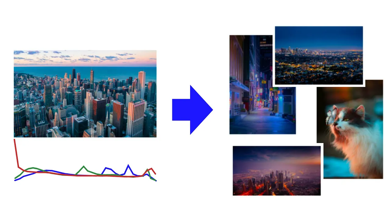
And we can see an example of what we're going to learn about here. So we have this query image, it's just a city, you can see it's very blue and orange, and to the right here, we have this, it was basically, this is what the color histogram is. Now, when we actually build our color histograms and search with them, we are going to convert them into a single vector, so an image embedding.

And with that image embedding, we're going to return these five images. Now, this is using a very small dataset. We have, I think it is literally 21 images, it's tiny. So with that in mind, this is returning pretty relevant images when we speak about the color content of these images.

They all seem to have this similar sort of aesthetic, a lot of blues and oranges. So this is pretty much what we're going to do. And underneath these images, you can actually see the color profiles as well. So the one to the right is actually just a duplicate image, it's the same image.

But then the other ones, we can see that they all have this kind of, or some of them have this peak in the red, and then they're pretty flat with the rest of the colors. So this example demonstrates the core idea of color histograms. That is, we take an image, translate it into the histograms that you saw, which we then translate into a image embedding vector, and then use our color profile embedding to retrieve other similar images based on their color profiles.

Now, there are many pros and cons to this technique. I mean, as you'd expect, it's one of the earliest techniques for image retrieval, but there are a lot of benefits. And we'll discuss a lot of those as we go through this video and just understand how to actually implement a color histogram.

It'll become quite clear what the pros and cons are, if you haven't figured a few of those out already. Now, we're going to work through two notebooks. The first one's just going to show us how we actually build color histograms, so we can actually see step by step the actual process.

And the second one is where we'll implement the search component. Now, you can find links to both of these notebooks in the description of this video. So if you want to follow along, go ahead, open those, and you'll be able to go through the code live. So a few things that we need to install.

So just pip install, we have OpenCV library, NumPy, and datasets. Now, OpenCV is just a public computer vision library. NumPy, I'm sure you probably know what it is. It's just focused on numerical operations for arrays. And datasets is HuggingFace datasets. HuggingFace is like an NLP library, and datasets is their way of allowing people to store datasets and download them super easily.

So for us, we are going to use that to get this image set here. Now, you can use your own images if you like. You don't have to do this one, but this is what I'm going to go with. And this is, like I said, it's, I think, 21 images.

It's really not that many, but it's all we need for this example. So you can load the dataset. So from datasets, load dataset, and we have this pinecone image set. If you'd like to see where this dataset is, you can go to HuggingFace.co/datasets, and then you just type in the dataset name that you see here, pinecone/image set.

And it will take you to where, yeah, this website here, which is where this dataset is actually hosted. Now inside, actually, let me run this. So inside here, we have this image bytes feature, and this is just a base 64 encoded representation of our image bytes. So when we download these, we need to decode them, again, using base 64.

So we do that here. So we're just going to create this processing function, and we're going to decode everything. I don't think there's really much to go through there, but from that, we'll get these images. Okay. And we can actually check. So let's just see how many images there are.

21. Okay. And this should align to appear as always number of rows 21. Okay. Cool. And we can display the images now with matplotlib. And you see we get this image with these three dogs, but they're pretty blue. That's because we have loaded them, or we've decoded them using the OpenCV library.

And OpenCV library, it reads images using the color channels, blue, green, and red in that order. And I don't know why they do that. It's kind of the opposite way of what most things do, which is red, green, and blue, or RGB. So what we need to do is actually flip those color channels if we'd like to see the true color version of this image.

So let me show you. So at the moment, this is a shape of that image. So this image is actually an array. These two here are like the actual pixel values. So you can see two, five, six, zero at the bottom here. And then you can see one, six, zero, zero over here.

Okay. So it's the Y, Y axis or the height of the image, and this is the width of the image. And then this three, these are the color channels. So it's the blue, green, and red color channels. And here are the color values. So blue, green, and red for the very top left pixel, right up there in the corner.

Okay. So we can see these values, by the way, so they go from zero, which is no color up to 255, which is full color. And we'll have a look at that in a moment. I'll show you what I mean. So first let's just flip those color channels. So you do NP flip.

We are going to flip the whole array, but we are going to flip it from axis two, which is a color channel axis. So let's do that. And you can see the shape is exactly the same because all we've done is flipped it, but these, the pixel values here, so it was blue, green, red is now red, green, blue.

So now we can visualize that and we actually get the actual picture, which is these three dobs that are very much not blue. So first we're going to go through building a histogram the slow way, just so we can understand exactly what is actually going on. So let's take a look at image zero again.

So the three dobs, and we're going to have a look at pixel zero. Okay. So we have those, those values. Again, this is the other way around. So it's blue, green, red. Now each pixel, like I said, has those blue, green, red activation values from zero, no color to two, five, five max color.

So if you had, let's say these were zero, zero, and zero, there's no color or there. That means we would get just black. Okay. Cause there's no color. If we had two, five, five, two, five, five, two, five, five, then we have white, which is just all the color you can possibly have in one.

Okay. And in between them, you have everything. So here's a few examples. We have blue, green, red, and a few other things. And I'm just going to plot those in this array here. And I'll show you. Okay. So we can see we have blue, green, red, and so on and so on.

Okay. And you can see all I'm doing is swapping the two, five, fives for the orange one. We've got like half of the green color in there as well, but that's pretty much all we're doing. So every single color can be represented by these values. So back to the previous values, we have that, the top left corner pixel of that picture of three doves, we have blue, green, and red.

So you can think, okay, blue, green, and red, that means it's going to be sort of a greeny blue color, which is going to be quite neutral because you have all of those colors kind of in the middle between zero and two, five, five. So we can see that here.

So this top left block here is actually that pixel, right? Because here, I'm just displaying the three by three pixels in the top left corner of the image. Okay. And this is a true color image, by the way, that's why it's RGB image. So that's the one we flipped.

Now what we are going to want to do when we're comparing these images is actually, we don't want an array, we want a vector. So I'm going to reshape this. Okay. And now we have these 409, or four and a little bit million values, which is just all of the rows in our image, or sorry, yeah, all the rows concatenated together.

Okay. That's what this reshape is doing. Now, if we plot that again, we can still see that those top three values are the same. Okay. But there's no more rows underneath those pixels anymore. It's just a single row. Okay. Now, okay, we have this one row, but it's still actually an array because we have the three color channels.

So we need to also extract those out. Okay. And now we literally just have three vectors that represent our image. And we can visualize each of these with a histogram. So let's do that. And this is the color profile, the red, green, and blue color profile of that image of the three dobs.

So what we have on the X axis here is the color activation value from zero up to 255. And then what we have on the Y axis here is the count of the number of pixels that have that particular value. So, I mean, we can see this is a pretty neutral color.

Okay. Most of the values, and this is probably the case for most images as well. Most of the values are kind of in the middle point. So it's pretty neutral. You can see that there's a lot of pixels here that don't have any blue in whatsoever. But beyond that, I don't think there's as much to note from there.

Okay. So let's put everything we've done so far into a single function so that we can replicate these charts for a few images. So what did we do before? We had our image. We can also change the number of bins that we use. So you see up here where we've got an individual bin for every single color activation value.

We can push those together so that we have less bins and we are going to do that later on because it doesn't really affect the retrieval performance that much unless you go really low. So first we're going to convert to a true color image. So from BGR to RGB, I'm just going to show the image so we can see what's actually happening whenever we call this function.

Convert it into a vector with the three channels. And then what we're going to do is, so here I'm breaking the values or dividing the values by the number of bins and then converting them back to integer values. This is basically just a really quick way of creating the bins.

So if I divided this by two, for example, so I had two bins here we'd get 128 in this division parameter. And we'd divide everything by 128. So we're kind of pushing everything together, all these pixel values into discrete categories or bins. And then we want to get the red, green, blue channels.

And then we plot it. So I'm going to run that and we're just going to try it on a few images. So we'll start with this one. So we have this image of a city and this is, I think, where you can see color histograms are a bit more interesting than the last one.

So it's a very blue image. And we can see that here, like it is super blue. And then we look at the histograms and the blue histogram, there's a lot of high values for blue pixels over here. Now, what you can also do, which I mentioned before, is use the bins parameter.

So we just want, let's say we want 64 bins here. And you can see that we have these sort of bars now where you can really see those before. That's because we have 64 values and we can reduce that even more. Let's say we wanted to go really low and we want to go to two.

Okay. And we just get these two bins now. Okay. And you can still see even from these two bins, it's a very blue image, but of course that's a little bit too much. So we'll stick with sort of values between 32, 64, because you can actually see what's going on with that.

Now, if you have a look at this image, we can see there's very little blue in this image. It's a lot of green, a little bit of red as well. If you take a look, we can see that almost all of the blue values are pushed right to the left, which means there's very few high value blue pixels in this image.

We can do this again here. We see, okay, again, it's very green. So don't really get those blues and we can keep going through all of that. See a few more. And this one, this one's also interesting because it's a very color specific image. It's a lot of orange there.

And you can kind of see that because it just got these really big spikes in particular areas of your histograms. So, well, we can see that represented by the histograms. Now that's a slow way of building histograms. Like I said before, we've gone through that to understand exactly what is going on, but it's not the most efficient way of doing it because there are already functions for creating histograms built into the OpenCV library.

So let's have a look at how we would use that. So we have this CV2, we've imported the CV library earlier, just here. So just import CV2. And then what we're going to do is we create, we use this calc_hist function. We pass in an image, we pass in the color channel.

We can only do this one color channel at a time. Whether you want to mask anything, I'll explain that in a minute and so on. I'll explain the rest in a moment as well. So we'll run that and you see that we get this 64 by 1 shape. And this is actually our histogram.

So we don't even need to use, before we're using matplotlib, the histogram function there. Now we don't even need to use that. We can just plot this directly. Now there are a few things in here. So we have this calc_hist function. What are all these values? So we have images, channels, mask_hist_size and ranges.

What does that mean exactly? So the images. So this is a list of CV2 loaded images with the channels blue, green and red. So if you look up here, that's why I've taken the red histogram from the third channel or position two and green obviously in one and blue in zero.

It can load multiple images. So that's why we have put that single image inside the square brackets, where is it? Here. And then we have channels. So this is what channels you want to create your histogram for. I'm wanting to extract one at a time here. So I've said, okay, I want the red channel or the channel in position two and so on.

Mask is another image or array which just consists of zeros and ones. Now that allows us to mask a part of the image if we would like to. So imagine you had half of the images zeros, half the image is ones. It means that you would literally remove half of the image when you add that mask to this.

Okay. Imagine you multiply all the values in your image by the zero ones, the ones that become zero there, you can't see them anymore because their color activations are zero. Okay. So they just become black. That's how it works. And then bins is the number of bins that we'd like to add in there like we did before.

And then the histogram range is the range of color values that we would expect because we're using RGB, we expect zero to 255. So rewrite zero to 256 because the top value is not inclusive. So that is not included. So actually just goes up to 255. Okay. And let's have a look at what we get from that.

So like I said, we don't need to use the histogram plot from that plot lib anymore. We can just plot it directly and yeah, we get this. Okay. So I think this is, is it the last image? Yeah. So it's this image here. You can see that we get the same thing.

So that's the end of the building histograms notebook. Let's have a look at how we actually create our embeddings with this and then how we actually search using these color histograms. Okay. So we're now in this search histogram notebook and what we're going to do is create a function to basically do everything we've done so far.

So using the CV2CalcHistForth function, we're going to use that. And then we're going to actually concatenate the red, green, and blue channels into a single vector. So you've seen this before. We have red, green, and blue. Then we concatenate red, green, and blue together along axis zero. And then we reshape.

So this is a minus one. That's just to remove, when you run this, there's always like an extra dimension in there. So we're just removing that extra dimension. Now, if we run that, we should see that we get this. So we have a 96 dimension vector. Now, why is it 96?

So we have, we just set the default number of bins to 32 at the top here. So that means we'll get 32 values for the red channel, for the green value and the blue channel, and then we concatenate them all together. So in the end, we have all those 32s together, three of them.

So we get a vector of dimension 96. So if you also imagine this, so let me visualize it even. So we run this. You can see here, we have the vector, the values from up to 32 here from 32 to 64, and from 64 to 96. And these are red, green, and blue.

And we get this. It's the same thing as what we saw before, but we just separated them all into a vector rather than a array with three color channels. Now let's go through and we'll just use this loop to do that for all of our images. So we're going to create all of these image vectors and we can compare vectors with Euclidean distance, although I found this didn't work very well, at least not compared to cosine similarity, which we calculated like this.

So what we're going to do is use cosine similarity to find the most similar matches for each image, and we're going to pull this within a function to keep everything clean. During visualization, we're also going to use the deflect arrays, so the true color arrays. So I can actually see what they are a little bit better.

So I'm going to run that. If I go through here, all we're doing, we're getting the query vector, which is marked by this index value here. So for example, those three dogs, they were position zero within our images. So if I wanted to use that as our query vector, I would just pass zero to this function here, and that will retrieve the query vector from the image vectors we've already created.

Now I'm going to go through and I'm going to calculate the distance between that query vector and that query image and every other vector within our image vectors. That also includes the same image. I mean, it's not hard to remove that from here, but just for the sake of simplicity, I've kept it in.

Plus it tells us if this is actually working, because we should always return that one as the most similar image. And then we're using this NumPy arg partition function, which is just based on the distances we calculate, it's going to retrieve those indexes. And then we can use those indexes to retrieve the images, the actual images themselves that are the most similar.

So if we just run that using the dog image, we see that we returned dog image first, because that's the, oh, sorry, this is reversed. So this is actually the first most similar image. And that is the dog image itself. And then we have these other ones. We didn't know what those are.

So let's go ahead. I'm going to write another function. This is not so important, but this just going to help us visualize these results. So I'm just, there's a lot of NumPy here. We don't really need to go through this, but you can go through this code if you want to.

So run that, and then I am going to get some results, same as what we saw before. And I just want to visualize those. So here I'm actually doing it for another image, so we can ignore that bit there. So for image six. Okay, cool. So we have, this is the image that we're using as our query.

And you can see, this is what I showed you at the start. So it's the city image. And we have these, this is the color histogram for it. And then these are the images that it's returning. So very similar in terms of the color scheme for each of these.

Let's try another one. Okay. So this one, I mean, it's pretty obvious what this should return, probably another image. As we can see, like that one. So we have this yellow background with the dog, and then we have the yellow background with a cat. Okay. And then there's some other images.

These ones are not really that similar, but there aren't that many images in this dataset. So that's why there aren't any others that are more similar. And this one, I think is really good because we can really see that these two color histograms are very aligned, like they're very similar.

And if we want to just have a look at, so at the moment we're using all of the, we're using a default number of bins. I'm not sure what the value is. Anyway, we can modify the number of bins. So we'll go 96. Let's see what we get. Okay.

And we get this. So now we're modifying the bins. We're still returning the same images. So there isn't, I think one of these might be slightly different. Okay. So this one here, actually reducing the number of bins here did damage the quality of this retrieval. So in this case, we still have that relevant image, but it's, we have these other images that are actually being placed before it, which is surprising, but it's just one of the limitations of this technique is it's not particularly robust.

Now this is, this is how we would actually search using these color histograms. Now I think it's probably quite clear what some limitations of this are. This retrieval technique isn't perfect. And I think these results highlight some of those drawbacks. So the key limitation here is like, okay, we come up here and we can see, yeah, we were getting, we're returning this image of a cat with a yellow background.

But what if for your use case, you're, you're not actually looking for the similar color. You're actually looking more for similar content. So you'd actually want to return, okay, this is a dog. I want to return another dog. So probably this image over here, in that case, this is a really bad technique because it's basing everything purely on the color.

It's not even looking, it's not looking at textures and not looking at the edges of an image. It's not looking at what is inside the image. It's just looking at the color profile of each image. So it's very limited with that. Now there was further work on color histograms to improve some of these.

So for example, different techniques that consider the texture of images, they consider the edges within the images and a few other things. But still all of these things, they're not going to get you as far as some of the more recent deep learning methods that allow you to actually consider what is inside the image from a very sort of human perspective.

But that being said, if you just want to return images or retrieve images that have a similar sort of aesthetic to a particular image that you're searching with, say even a similar color profile, like we saw with the earlier results up here, we are returning pictures that kind of look like the first image, like the query image.

So that's one pro to using this technique. Another one is that it's incredibly easy to implement. We've just done it. And in reality, we don't even need to go through that sort of slow building a histogram part. We can just do it super quickly using OpenCV. And another key benefit is the results are very interpretable.

So with a lot of deep learning methods, you have a black box, you put in some data, you return some results. Why did you get those results? A lot of the time you don't really know. With this, you know exactly why you're returning a particular result. You can see that the color profile is very similar to the one, the particular color profile that you're querying with.

So we understand why that's actually happening here. It's not a black box like neural networks. So with all that in mind, this approach to image embedding and retrieving images is great if your use case is looking at the aesthetics or the color profile of images. If you want something more advanced, of course, you're going to want to go for something else.

Now that's it for this video. I hope this sort of introduction to 1D earlier, image embedding techniques and methods for content-based image retrieval has been interesting. But for now, we're going to leave it there. So thank you very much for watching and I will see you again in the next one.

Bye.