So, welcome back everybody. Thanks for coming and I hope you had a good week and had a fun time playing around with artistic style. I know I did. I thought I'd show you. So I tried a couple of things myself over the week with this artistic style stuff. I've just tried a couple of simple little changes which I thought you might be interested in.

One thing before I talk about the artistic style is I just wanted to point out some of the really cool stuff that people have been contributing over the week. If you haven't come across it yet, be sure to check out the wiki. There's a nice thing in Discourse where you can basically set any post as being a wiki, which means that anybody can edit it.

So I created this wiki post early on, and by the end of the week we now have all kinds of stuff with links to the stuff from the class, a summary of the paper, examples, a list of all the links, both snippets, a handy list of steps that are necessary when you're doing style transfer, lots of stuff about the TensorFlow Dead Summit, and so forth.

Lots of other threads. One I saw just this afternoon popped up, which was Greg from XinXin, talked about trying to summarize what they've learned from lots of other threads across the forum. This is a great thing that we can all do is when you look at lots of different things and take some notes, if you put them on the forum for everybody else, this is super handy.

So if you haven't quite caught up on all the stuff going on in the forum, looking at this curating lesson 8 experiments thread would be probably a good place to start. So a couple of little changes I made in my experiments. I tried thinking about how depending on what your starting point is for your optimizer, you get to a very different place.

And so clearly our convex optimization is not necessarily finding a local minimum, but at least saddle points it's not getting out of. So I tried something which was to take the random image and just add a Gaussian blur to it. So that makes a random image into this kind of thing.

And I just found that even the plain style looked a lot smoother, so that was one change that I made which I thought worked quite well. Another change that I made just to play around with it was that I added a different weight to each of the style layers.

And so my zip now has a third thing in which is the weights, and I just multiply by the weight. So I thought that those two things made my little bird look significantly better than my little bird looked before, so I was happy with that. You could do a similar thing for content loss.

You could also maybe add more different layers of content loss and give them different weights as well. I'm not sure if anybody's tried that yet. Yes, Rachel. I have a question in regards to style transfer for cartoons. With cartoons, when we think of transferring the style, what we really mean is transferring the contours of the cartoon to redraw the content in that style.

This is not what style transferring is doing here. How might I implement this? I don't know that anybody has quite figured that out, but I'll show you a couple of directions that may be useful. I've tried selecting activations that correspond with edges, and such is indicated by one of the calm visualization papers and comparing outputs from specifically those activations.

So I'll show you some things you could try. I haven't seen anybody do a great job of this yet, but here's one example from the forum. Somebody pointed out that this cartoon approach didn't work very well with Dr. Seuss, but then when they changed their initial image not to be random but to be the picture of the dog, it actually looked quite a lot better.

So there's one thing you could try. There's some very helpful diagrams that somebody posted which is fantastic. I like this summary of what happens if you add versus remove each layer. So this is what happens if you remove block 0, block 1, block 2, block 3, and block 4 to get a sense of how they impact things.

You can see for the style that the last layer is really important to making it look good, at least for this image. One of you had some particularly nice examples. It seems like there's a certain taste. They're kind of figuring out what photos go with what images. I thought this Einstein was terrific.

I thought this was terrific as well. Brad came up with this really interesting insight that starting with this picture and adding a style to it creates this extraordinary shape here where, as he points out, you can tell it's a man sitting in the corner, but there's less than 10 brush strips.

Sometimes this style transfer does things which are surprisingly fantastic. I have no idea what this is even in the photos, so I don't know what it is in the painting either. I guess I don't watch that kind of music enough. So there's lots of interesting ideas you can try, and I've got a link here, and you might have seen it in the PowerPoint, to a Keras implementation that has a whole list of things that you can try.

Here are some particular examples. All of these examples you can get the details from this link. There's something called chain blurring. For some things, this might work well for cartoons. Notice how the matrix doesn't do a good job with the cat when you use the classic This Is Our Paper.

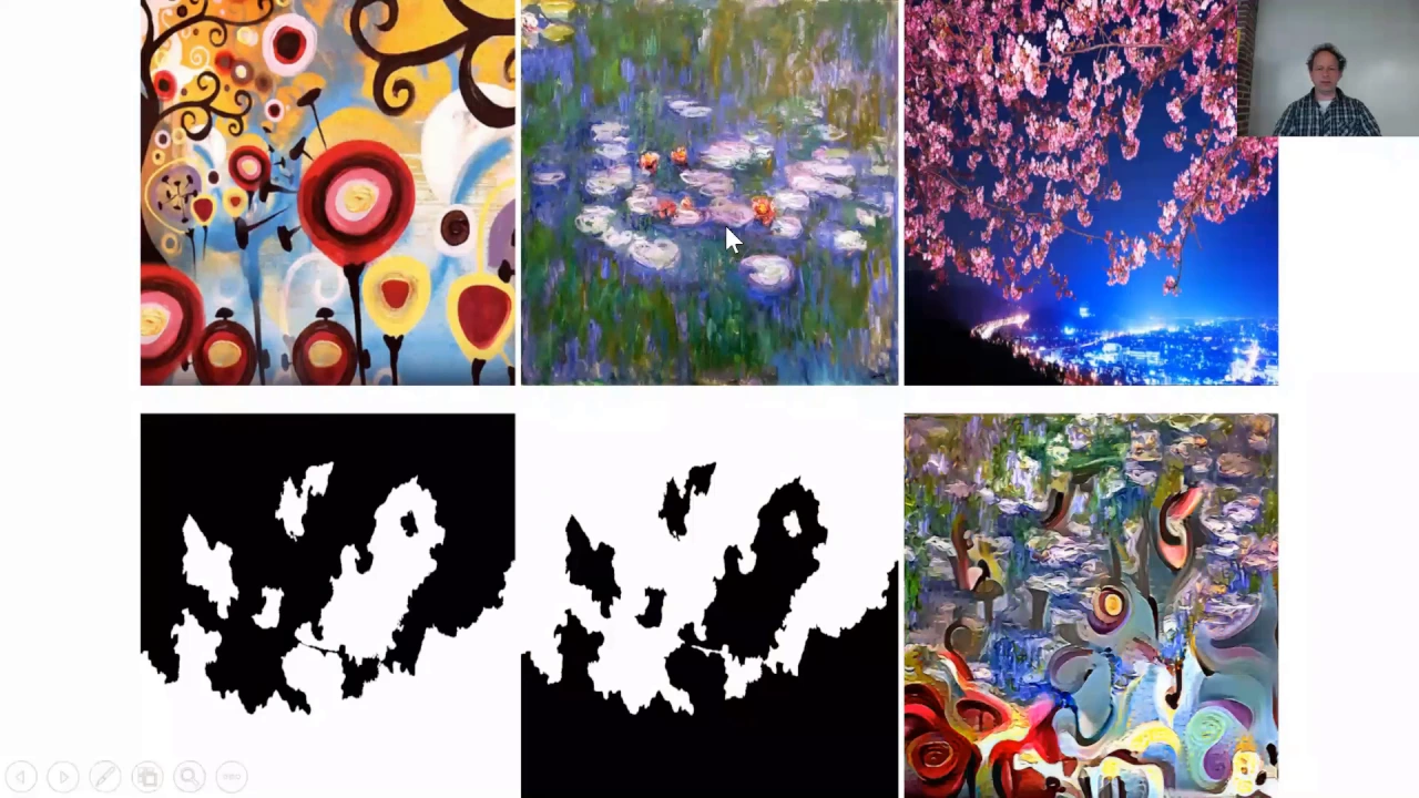
But if you use this chain blurring approach, it does a fantastic job. So I wonder if that might be one secret to the cartoons. Some of you I saw in the forum have already tried this, which is using color preservation and luminance matching, which basically means you're still taking the style but you're not taking the color.

And I think in these particular examples, this is really great results. I think it depends a lot on what things you tried with. You can go a lot further. For example, you can add a mask and then say just do color preservation for one part of the photo. So here the top part of the photo has got color preservation and the bottom hasn't.

They even show in that code how you can use a mask to say one part of my image should not be stylized. This is really crazy. Use masks to decide which one of two style images to use and then you can really generate some creative stuff. So there's a lot of stuff that you can play with and you can go beyond this to coming up with your own ideas.

Now some of the best stuff, you're going to learn a bit more today about how to do some of these things better. But just to give an idea, if you go to likemo.net, you can literally draw something using four colors and then choose a style image and it will turn your drawing into an image.

Basically the idea is blue is going to be water and green is going to be foliage and I guess red is going to be foreground. There's a lot of good examples of this kind of neural doodle they call it online. Something else we'll learn more about how to do better today is if you go to affinelayer.com, there's a very recent paper called Pics2Pics.

We're going to be learning quite a bit in this class about how to do segmentation, which is where you take a photo and turn it into a colored image, basically saying the horse is here, the bicycle is here, the person is here. This is basically doing the opposite. You start by drawing something, saying I want you to create something that has a window here and a window still here and a draw here and a column there, and it generates a photo, which is fairly remarkable.

So the stuff we've learned so far won't quite get you to do these two things, but by the end of today we should be able to. This is a nice example that I think some folks at Adobe built showing that you could basically draw something and it would try and generate an image that was close to your drawing where you just needed a small number of lines.

Again we'll link to this paper from the resources. This actually shows it to you in real time. You can see that there's some new way of doing art that's starting to appear where you don't necessarily need a whole lot of technique. I'm not promising it's going to turn you into a Van Gogh, but you can at least generate images that maybe are in your head in some style that's somewhat similar to somebody else's.

I think it's really interesting. One thing I was thrilled to see is that at least two of you have already written blog posts on Medium. That was fantastic to see. So I hope more of you might try to do that this week. It definitely doesn't need to be something that takes a long time.

I know some of you are also planning on turning your forum posts into blog posts, so hopefully we'll see a lot more blog posts this week popping up. I know the people who have done that have found that a useful experience as well. One of the things that I suggested doing pretty high on the list of priorities for this week's assignment was to go through the paper knowing what it's going to say.

I think this is really helpful is when you already know how to do something is to go back over that paper, and this is a great way to learn how to read papers. You already know what it's telling you. This is like the way I learnt to read papers was totally this method.

So I've gone through and I've highlighted a few key things which as I went through I thought were kind of important. In the abstract of the paper, let me ask, how many people kind of went back and relooked at this paper again? Quite a few of you, that's great.

In the abstract, they basically say what is it that they're introducing. It's a system based on a deep neural network that creates artistic images of higher perceptual quality. So we're going to read this paper and hopefully at the end of it we'll know how to do that. Then in the first section, they tell us about the basic ideas.

When CNNs are trained on object recognition, they developed a representation of an image. Along the processing hierarchy of the network, it's transformed into representations that increasingly care about the actual content compared to the pixel values. So it describes the basic idea of content loss. Then they describe the basic idea of style loss, which is looking at the correlations between the different filter responses over the spatial extent of the feature maps.

This is one of these sentences that read on its own doesn't mean very much, but now that you know how to do it, you can read it and you can see what that means, and then when you get to the methods section, we learn more. So the idea here is that by including the feature correlations, and this answers one of the questions that one of you had on the forum, by including feature correlations of multiple layers, we obtain a multi-scale representation of the input image.

This idea of a multi-scale representation is something we're going to be coming across a lot because a lot of this, as we discussed last week, a lot of this class is about generative models. One of the tricky things with generative models is both to get the general idea of the thing you're trying to generate correct, but also get all the details correct.

So the details generally require you to zoom into a small scale, and the big picture correct is about zooming out to a large scale. So this was one of the key things that they did in this paper was show you how to create a style representation that included multiple resolutions.

We now know that where they did that was to use multiple style layers, and as we go through the layers of VGG, they gradually become lower and lower resolution, larger and larger receptive fields. I'm always great to look at the figures and make sure I was thrilled to see that some of you were trying to recreate these figures, which actually turned out to be slightly non-trivial.

So we can see exactly what that figure is, and if you haven't tried it for yourself yet, you might want to try it, see if you can recreate this figure. It's good to try and find in a paper the key thing that they're showing. In this case, they found that representations of content and style in a CNN are separable, and you can manipulate both to create new images.

So again, hopefully now you can look at that and say, Oh yeah, that makes sense. You can see that with papers, certainly with this paper, there's often quite a lot of introduction that often says the same thing a bunch of different ways. The first time you read it, one paragraph might not make sense, but later on they say it a different way and it starts to make more sense.

So it's worth looking through the introductory remarks, maybe two or three times. They can certainly see that again, talking about the different layers and how they behave. Again, showing the results of some experiments. Again, you can see if you can recreate these experiments, make sure you understand how to do it.

And then there's a whole lot of stuff I didn't find that interesting until we get to the section called methods. So the method section is the section that hopefully you'll learn the most about reading papers after you've implemented something by reading the section called methods. I want to show you a few little tricks of notation.

You do need to be careful of little details that fly by. Like here, they used average pooling. That's a sentence which if you weren't reading carefully, you could skip over it. We need to use average pooling, not math pooling. So they will often have a section which explicitly says, Now I'm going to introduce the notation.

This paper doesn't. This paper just introduces the notation as part of the discussion. But at some point, you'll start getting Greek letters or things with subscripts or whatever. Notation starts appearing. And so at this point, you need to start looking very carefully. And at least for me, I find I have to go back and read something many times to remember what's L, what's M, what's N.

This is the annoying thing with math notation, is they're single letters. They generally don't have any kind of mnemonic. Often though you'll find that across papers in a particular field, they'll tend to reuse the same kind of English and Greek letters for the same kinds of things. So M will generally be the number of rows, capital M.

Capital N will often be the number of columns. K will often be the index that you're summing over, so on and so forth. So here, the first thing which is introduced is x with an arrow on top. So x with an arrow on top means it's a vector. It's actually an input image, but they're going to turn it into a vector by flattening it out.

So our image is called x. And then the CNN has a whole bunch of layers, and every time you see something with a subscript or a superscript like this, you need to look at both of the two bits because they've both got a meaning. The big thing is like the main object.

So in this case, capital N is a filter. And then the subscript or superscript is like in an array or a tensor. In Python, it's like the thing in square brackets. So each filter has a letter l, which is like which number of the filter is it. And so often as I read a paper, I'll actually try to write code as I go and put little comments so that I'll write layer, square bracket, layer number, plus square bracket, and then I have a comment after, say, ml, just to remind myself.

So I'm creating the code and mapping it to the letters. So there are nl filters. We know from a CNN that each filter creates a feature map, so that's why there are nl feature maps. So remember, any time you see the same letter, it means the same thing within a paper.

Each feature map is of size m, and as I mentioned before, m tends to be rows and m tends to be columns. So here it says m is the height times the width of the feature map. So here we can see they've gone .flat, basically, to make it all 1 row.

Now this is another piece of notation you'll see all the time. A layer l can be stored in a matrix called f, and now the l has gone to the top. Same basic idea, just an index. So the matrix f is going to contain our activations. And this thing here where it says r with a little superscript has a very special meaning.

It's referring to basically what is the shape of this. So when you see this shape, it says these are r means that they're floats, and this thing here means it's a matrix. You can see the x, so it means it's rows by a column. So there are n rows and m columns in this matrix, and every matrix, there's one matrix for each layer, and there's a different number of rows and different number of columns for each layer.

So you can basically go through and map it to the code that you've already written. So I'm not going to read through the whole thing, but there's not very much here, and it would be good to make sure that you understand all of it, perhaps with the exception of the derivative, because we don't care about derivatives because they get done for us thanks to a theano-intensor flow.

So you can always skip the bits about derivatives. So then they do the same thing basically describing the Gram matrix. So they show here that the basic idea of the Gram matrix is that they create an inner product between the vectorized feature map i and j. So vectorized here means turned into a vector, so the way you turn a matrix into a vector is flattened.

This means the inner product between the flattened feature maps, so those matrices we saw. So hopefully you'll find this helpful. You'll see there will be small little differences. So rather than taking the mean, they use here the sum, and then they divide back out the number of rows and columns to create the mean this way.

In our code, we actually put the division inside the sum, so you'll see these little differences of how we implement things. And sometimes you may see actual meaningful differences, and that's often a suggestion of something you can try. So that describes the notation and the method, and that's it.

But then very importantly, any time you come across some concept which you're not familiar with, it will pretty much always have a reference, a citation. So you'll see there's little numbers all over the place. There's lots of different ways of doing these references. But anytime you come across something which has a citation, like a new piece of notation or a new concept, you don't know what it is.

Generally the first time I see it in a paper, I ignore it. But if I keep reading and it turns out to be something that actually is important and I can't understand the basic idea at all, I generally then put this paper aside, I put it in my to-read file, and make the new paper I'm reading the thing that it's citing.

Because very often a paper is entirely meaningless until you've read one or two of the key papers it's based on. Sometimes this can be like reading the dictionary if you don't get low English. It can be layer upon layer of citations, and at some point you have to stop.

I think you should find that the basic set of papers that things refer to is pretty much all stuff you guys know at this point. So I don't think you're going to get stuck in an infinite loop. But if you ever do, let us know in the forum and we'll try to help you get unstuck.

Or if there's any notation you don't understand, let us know. In other words, the horrible things about math is it's very hard to search for. It's not like you can take that function name and search for Python and the function name instead of some weird squiggly shape. So again, feel free to ask if you're not sure about that.

There is a great Wikipedia page which lists, I think it's just called math notation or something, which lists pretty much every piece of notation. There are various places you can look up notation as well. So that's the paper. Let's move to the next step. So I think what I might do is kind of try and draw the basic idea of what we did before so that I can draw the idea of what we're going to do differently this time.

So previously, and now this thing is actually calibrated, we had a random image and we had a loss function. It doesn't matter what the loss function was. We know that it happened to be a combination of style_loss plus content_loss. What we did was we took our image, our random image, and we put it through this loss function and we got out of it two things.

One was the loss and the other was the gradients. And then we used the gradients with respect to the original pixels to change the original pixels. So we basically repeated that loop again and again, and the pixels gradually changed to make the loss go down. So that's the basic approach that we just used.

It's a perfectly fine approach for what it is. And in fact, if you are wanting to do lots of different photos with lots of different styles, like if you created a web app where you said please upload any style image and any content image, here's your artistic style version, this is probably still the best, particularly with some of those tweaks I talked about.

But what if you wanted to create a web app that was a Van Gogh irises generator? Upload any image and I will give you that image in the style of Van Gogh's irises. You can do better than this approach, and the reason you can do better is that we can do something where you don't have to do a whole optimization run in order to create that output.

Instead, we can train a CNN to learn to output photos in the style of Van Gogh's irises. The basic idea is very similar. What we're going to do this time is we're going to have lots of images. We're going to take each image and feed it into the exact same loss function that we used before, with the style loss plus the content loss.

For the style loss, we're going to use Van Gogh's irises, and for the content loss, we're going to use the image that we're currently looking at. What we do is rather than changing the pixels of the original photo, instead what we're going to do is we're going to train a CNN to take this out of the way.

Let's put a CNN in the middle. These are the layers of the CNN. We're going to try and get that CNN to spit out a new image. There's an input image and an output image. This new CNN we've created is going to spit out an output image that when you put it through this loss function, hopefully it's going to give a small number.

If it gives a small number, it means that the content of this photo still looks like the original photo's content, and the style of this new image looks like the style of Van Gogh's irises. So if you think about it, when you have a CNN, you can really pick any loss function you like.

We've tended to use pretty simple loss functions so far like mean squared error or cross entropy. In this case, we're going to use a very different loss function which is going to be style plus content loss using the same approach that we used just before. And because that was generated by a neural net, we know it's differentiable.

And you can optimize any loss function as long as the loss function is differentiable. So if we now basically take the gradients of this output, not with respect to the input image, but with respect to the CNN weights, then we can take those gradients and use them to update the weights of the CNN so that the next iteration through the CNN will be slightly better at turning that image into a picture that has a good style match with Van Gogh's irises.

Does that make sense? So at the end of this, we run this through lots of images. We're just training a regular CNN, and the only thing we've done differently is to replace the loss function with the style_loss plus content_loss that we just used. And so at the end of it, we're going to have a CNN that has learnt to take any photo and will spit out that photo in the style of Van Gogh's irises.

And so this is a win, because it means now in your web app, which is your Van Gogh's irises generator, you now don't have to run an optimization path on the new photo, you just do a single forward pass to a CNN, which is instant. This is going to limit the filters you use, let's say you have Photoshop and you want to change multiple styles.

Yeah, this is going to do just one type of style. Is there a way of combining multiple styles, or is it just going to be a combination of all of them? You can combine multiple styles by just having multiple bits of style loss for multiple images, but you're still going to have the problems that that network has only learned to create one kind of image.

It may be possible to train it so it takes both a style image and a content image, but I don't think I've seen that done yet. Having said that, there is something simpler and in my opinion more useful we can do, which is rather than doing style loss plus content loss.

Let's think of another interesting problem to solve, which is called super resolution. Super resolution is something which, honestly, when Rachel and I started playing around with it a while ago, nobody was that interested in it. But in the last year or so it's become really hot. So we were kind of playing around with it quite a lot, we thought it was really interesting but suddenly it's got hot.

The basic idea of super resolution is you start off with a low-res photo. The reason I started getting interested in this was I wanted to help my mom take her family photos that were often pretty low quality and blow them up into something that was big and high quality that she could print out.

So that's what you do. You try to take something which starts with a small low-res photo and turns it into a big high-res photo. Now perhaps you can see that we can use a very similar technique for this. What we could do is between the low-res photo and the high-res photo, we could introduce a CNN.

That CNN could look a lot like the CNN from our last idea, but it's taking in as input a low-res image, and then it's sticking it into a loss function, and the loss function is only going to calculate content loss. The content loss it will calculate is between the input that it's got from the low-res after going through the CNN compared to the activations from the high-res.

So in other words, has this CNN successfully created a bigger photo that has the same activations as the high-res photo does? And so if we pick the right layer for the high-res photo, then that ought to mean that we've constructed a new image. This is one of the things I wanted to talk about today.

In fact, I think it's at the start of the next paper we're going to look at is they even talk about this. This is the paper we're going to look at today, Perceptual Losses for Real-Time Style Transfer and Super Resolutions. This is from 2016. So it took about a year or so to go from the thing we just saw to this next stage.

What they point out in the abstract here is that people had done super resolution with CNNs before, but previously the loss function they used was simply the mean-squared error between the pixel outputs of the upscaling network and the actual high-res image. The problem is that it turns out that that tends to create blurry images.

It tends to create blurry images because the CNN has no reason not to create blurry images. Blurry images actually tend to look pretty good in the loss function because as long as you get the general, oh this is probably somebody's face, I'll put a face color here, then it's going to be fine.

Whereas if you take the second or third conv block of VGG, then it needs to know that this is an eyeball or it's not going to look good. So if you do it not with pixel loss, but with the content loss we just learned about, you're probably going to get better results.

Like many papers in deep learning, this paper introduces its own language. In the language of this paper, perceptual loss is what they call the mean-squared errors between the activations of a network with two images. So the thing we've been calling content loss, they call perceptual loss. So one of the nice things they do at the start of this, and I really like it when papers do this, is to say why is this paper important?

Well this paper is important because many problems can be framed as image transformation tasks, where a system receives some input and chucks out some other output. For example, denoising. Learn to take an input image that's full of noise and spit out a beautifully clean image. Super resolution, take an input image which is low-res and spit out a high-res.

Colorization, take an input image which is black and white and spit out something which is color. Now one of the interesting things here is that all of these examples, you can generate as much input data as you like by taking lots of images, which are either from your camera or you download off the internet or from ImageNet, and you can make them lower-res.

You can add noise. You can make them black and white. So you can generate as much labeled data as you like. That's one of the really cool things about this whole topic of generators. With that example, going to lower-res imagery, it's algorithmically done. Is the neural net only going to learn how to transfer out something that's algorithmically done versus an actual low-res imagery that doesn't have like -- So one thing I'll just mention is the way you would create your labeled data is not to do that low-res on the camera.

You would grab the images that you've already taken and make them low-res just by doing filtering in OpenCV or whatever. That is algorithmic, and it may not be perfect, but there's lots of ways of generating that low-res image. So there's lots of ways of creating a low-res image. Part of it is about how do you do that creation of the low-res image and how well do you match the real low-res data you're going to be getting.

But in the end, in this case, things like low-resolution images or black and white images, it's so hard to start with something which could be like -- I've seen versions with just an 8x8 picture and turning it into a photo. It's so hard to do that regardless of how that 8x8 thing was created that often the details of how the low-res image was created don't really matter too much.

There are some other examples they mention which is turning an image into an image which includes segmentation. We'll learn more about this in coming lessons, but segmentation refers to taking a photo of something and creating a new image that basically has a different color for each object. Horses are green, cars are blue, buildings are red, that kind of thing.

That's called segmentation. As you know from things like the fisheries competition, segmentation can be really important as a part of solving other bigger problems. Another example they mention here is depth estimation. There are lots of important reasons you would want to use depth estimation. For example, maybe you want to create some fancy video effects where you start with a flat photo and you want to create some cool new Apple TV thing that moves around the photo with a parallax effect as if it was 3D.

If you were able to use a CNN to figure out how far away every object was automatically, then you could turn a 2D photo into a 3D image automatically. Taking an image in and sticking an image out is kind of the idea in computer vision at least of generative networks or generative models.

This is why I wanted to talk a lot about generative models during this class. It's not just about artistic style. Artistic style was just my sneaky way of introducing you to the world of generative models. Let's look at how to create this super resolution idea. Part of your homework this week will be to create the new approach to style transfer.

I'm going to build the super resolution version, which is a slightly simpler version, and then you're going to try and build on top of that to create the style transfer version. Make sure you let me know if you're not sure at any point. I've already created a sample of 20,000 image images, and I've created two sizes.

One is 288x288, and one is 72x72, and they're available as bcols arrays. I actually posted the link to these last week, and it's on platform.fast.ai. So we'll open up those bcols arrays. One trick you might have hopefully learned in part 1 is that you can turn a bcols array into a numpy array by slicing it with everything.

Any time you slice a bcols array, you get back a numpy array. So if you slice everything, then this turns it into a numpy array. This is just a convenient way of sharing numpy arrays in this case. So we've now got an array of low resolution images and an array of high resolution images.

So let me start maybe by showing you the final network. Okay, this is the final network. So we start off by taking in a batch of low-res images. The very first thing we do is stick them through a convolutional block with a stride of 1. This is not going to change its size at all.

This convolutional block has a filter size of 9, and it generates 64 filters. So this is a very large filter size. Particularly nowadays, filter sizes tend to be 3. Actually in a lot of modern networks, the very first layer is very often a large filter size, just the one, just one very first layer.

And the reason is that it basically allows us to immediately increase the receptive field of all of the layers from now on. So by having 9x9, and we don't lose any information because we've gone from 3 channels to 64 filters. So each of these 9x9 convolutions can actually have quite a lot of information because you've got 64 filters.

So you'll be seeing this quite a lot in modern CNN architectures, just a single large filter conv layer. So this won't be unusual in the future. Now the next thing, I'm going to give the green box behind you. Oh, just a moment, sorry. The stride 1 is also pretty popular, I think.

Well the stride 1 is important for this first layer because you don't want to throw away any information yet. So in the very first layer, we want to keep the full image size. So with the stride 1, it doesn't change, it doesn't downsample at all. But there's also a lot of duplication, right?

Like 9 filter size and 1 filter size? They overlap a lot, absolutely. But that's okay. A good implementation of a convolution is going to hopefully memoize some of that, or at least keep it in cache. So it hopefully won't slow it down too much. One of the discussions I was just having during the break was how practical are the things that we're learning at the moment compared to part 1 where everything was just designed entirely to be the most practical things which we have best practices for.

And the answer is a lot of the stuff we're going to be learning, no one quite knows how practical it is because a lot of it just hasn't really been around that long and isn't really that well understood and maybe there aren't really great libraries for it yet. So one of the things I'm actually hoping from this part 2 is by learning the edge of research stuff or beyond amongst a diverse group is that some of you will look at it and think about whatever you do 9 to 5 or 8 to 6 or whatever and think, oh, I wonder if I could use that for this.

If that ever pops into your head, please tell us. Please talk about it on the forum because that's what we're most interested in. It's like, oh, you could use super-resolution for blah or depth-finding for this or generative models in general for this thing I do in pathology or architecture or satellite engineering or whatever.

So it's going to require some imagination sometimes on your part. So often that's why I do want to spend some time looking at stuff like this where it's like, okay, what are the kinds of things this can be done for? I'm sure you know in your own field, one of the differences between expert and beginner is the way an expert can look at something from first principles and say, okay, I could use that for this totally different thing which has got nothing to do with the example that was originally given to me because I know the basic steps are the same.

That's what I'm hoping you guys will be able to do is not just say, okay, now I know how to do artistic style. Are there things in your field which have some similarities? We were going to talk about the super-resolution network. We talked about the idea of the initial conv block.

After the initial conv block, we have the computation. In any kind of generative network, there's the key work it has to do, which in this case is starting with a low-res image, figure out what might that black dot be. Is it a label or is it a wheel? Basically if you want to do really good upscaling, you actually have to figure out what the objects are so you know what to draw.

That's kind of like the key computation this CNN is going to have to learn to do. In generative models, we generally like to do that computation at a low resolution. There's a couple of reasons why. The first is that at a low resolution there's less work to do so the computation is faster.

But more importantly, at higher resolutions it generally means we have a smaller receptive field. It generally means we have less ability to capture large amounts of the image at once. If you want to do really great computations where you recognize that this blob here is a face and therefore the dot inside it is an eyeball, then you're going to need enough of a receptive field to cover that whole area.

Now I noticed a couple of you asked for information about receptive fields on the forum thread. There's quite a lot of information about this online, so Google is your friend here. But the basic idea is if you have a single convolutional filter of 3x3, the receptive field is 3x3.

So it's how much space can that convolutional filter impact. On the other hand, what if you had a 3x3 filter which had a 3x3 filter as its input? So that means that the center one took all of this. But what did this one take? Well this one would have taken, depending on the stride, probably these ones here.

And this one over here would have taken these ones here. So in other words, in the second layer, assuming a stride of 1, the receptive field is now 5x5, not 3x3. So the receptive field depends on two things. One is how many layers deep are you, and the second is how much did the previous layers either have a nonunit stride or maybe they had max pooling.

So in some way they were becoming down sampled. Those two things increased the receptive field. And so the reason it's great to be doing layer computations on a large receptive field is that it then allows you to look at the big picture and look at the context. It's not just edges anymore, but eyeballs and noses.

So in this case, we have four blocks of computation where each block is a ResNet block. So for those of you that don't recall how ResNet works, it would be a good idea to go back to Part 1 and review. But to remind ourselves, let's look at the code.

Here's a ResNet block. So all a ResNet block does is it takes some input and it does two convolutional blocks on that input, and then it adds the result of those convolutions back to the original input. So you might remember from Part 1 we actually drew it. We said there's some input and it goes through two convolutional blocks and then it goes back and is added to the original.

And if you remember, we basically said in that case we've got y equals x plus some function of x, which means that the function equals y minus x and this thing here is a residual. So a whole stack of residual blocks, ResNet blocks on top of each other can learn to gradually get thrown in on whatever it's trying to do.

In this case, what it's trying to do is get the information it's going to need to upscale this in a smart way. So we're going to be using a lot more of this idea of taking blocks that we know work well for something and just reusing them. So then what's a conv block?

All a conv block is in this case is it's a convolution followed by a batch norm, optionally followed by an activation. And one of the things we now know about ResNet blocks is that we generally don't want an activation at the end. That's one of the things that a more recent paper discovered.

So you can see that for my second conv block I have no activation. I'm sure you've noticed throughout this course that I refactor my network architectures a lot. My network architectures don't generally list every single layer, but they're generally functions which have a bunch of layers. A lot of people don't do this.

A lot of the architectures you find online are like hundreds of lines of layer definitions. I think that's crazy. It's so easy to make mistakes when you do it that way, and so hard to really see what's going on. In general, I would strongly recommend that you try to refactor your architectures so that by the time you write the final thing, it's half a page.

You'll see plenty of examples of that, so hopefully that will be helpful. So we've increased the receptive field, we've done a bunch of computation, but we still haven't actually changed the size of the image, which is not very helpful. So the next thing we do is we're going to change the size of the image.

And the first thing we're going to learn is to do that with something that goes by many names. One is deconvolution, another is transposed convolutions, and it's also known as fractionally strided convolutions. In Keras they call them decomvolutions. And the basic idea is something which I've actually got a spreadsheet to show you.

The basic idea is that you've got some kind of image, so here's a 4x4 image, and you put it through a 3x3 filter, a convolutional filter, and if you're doing valid convolutions, that's going to leave you with a 2x2 output, because here's one 3x3, another 3x3, and four of them.

So each one is grabbing the whole filter and the appropriate part of the data. So it's just a standard 2D convolution. So we've done that. Now let's say we want to undo that. We want something which can take this result and recreate this input. How would you do that?

So one way to do that would be to take this result and put back that implicit padding. So let's surround it with all these zeros such that now if we use some convolutional filter, and we're going to put it through this entire matrix, a bunch of zeros with our result matrix in the middle, and then we can calculate our result in exactly the same way, just a normal convolutional filter.

So if we now use gradient descent, we can look and see, what is the error? So how much does this pixel differ from this pixel? And how much does this pixel differ from this pixel? And then we add them all together to get our mean squared error. So we can now use gradient descent, which hopefully you remember from Part 1 in Excel is called solver.

And we can say, set this cell to a minimum by changing these cells. So this is basically like the simplest possible optimization. Solve that, and here's what it's come up with. So it's come up with a convolutional filter. You'll see that the result is not exactly the same as the original data, and of course, how could it be?

We don't have enough information, we only have 4 things to try and regenerate 16 things. But it's not terrible. And in general, this is the challenge with upscaling. When you've got something that's blurred and down-sampled, you've thrown away information. So the only way you can get information back is to guess what was there.

But the important thing is that by using a convolution like this, we can learn those filters. So we can learn how to up-sample it in a way that gives us the loss that we want. So this is what a deconvolution is. It's just a convolution on a padded input.

Now in this case, I've assumed that my convolutions had a unit strived. There was just 1 pixel between each convolution. If your convolutions are of strived 2, then it looks like this picture. And so you can see that as well as putting the 2 pixels around the outside, we've also put a 0 pixel in the middle.

So these 4 cells are now our data cells, and you can then see it calculating the convolution through here. I strongly suggest looking at this link, which is where this picture comes from. And in turn, this link comes from a fantastic paper called the Convolution Arithmetic Guide, which is a really great paper.

And so if you want to know more about both convolutions and deconvolutions, you can look at this page and it's got lots of beautiful animations, including animations on transposed convolutions. So you can see, this is the one I just showed you. So that's the one we just saw in Excel.

So that's a really great site. So that's what we're going to do first, is we're going to do deconvolutions. So in Keras, a deconvolution is exactly the same as convolution, except with DE on the front. You've got all the same stuff. How many filters do you want? What's the size of your filter?

What's your stride or subsample, as they call it? Border mode, so close. We have a question. If TensorFlow is the backend, shouldn't the batch normalization axis equals negative 1? And then there was a link to a GitHub conversation where Francois said that for Theano, axis is 1. No, it should be.

And in fact, axis minus 1 is the default. So, yes. Thank you. Well spotted. Thank David Gutmann. He is also responsible for some of our beautiful pictures we saw earlier. So let's remove axis. That will make things look better. And go faster as well. So just in case you weren't clear on that, you might remember from part 1 that the reason we had that axis equals 1 is because in Theano that was the channel axis.

So we basically wanted not to throw away the xy information, the batch normal across channels. In Theano, channel is now the last axis. And since minus 1 is the default, we actually don't need that. So that's our deconvolution blocks. So we're using a stride of 2,2. So that means that each time we go through this deconvolution, it's going to be doubling the size of the image.

For some reason I don't fully understand it and haven't really looked into it. In Keras, you actually have to tell it the shape of the output. So you can see here, you can actually see it's gone from 72x72 to 144x144 to 288x288. So because these are convolutional filters, it's learning to upscale.

But it's not upscaling with just three channels, it's upscaling with 64 filters. So that's how it's able to do more sophisticated stuff. And then finally, we're kind of reversing things here. We have another 9x9 convolution in order to get back our three channels. So the idea is we previously had something with 64 channels, and so we now want to turn it into something with just three channels, the three colors, and to do that we want to use quite a bit of context.

So we have a single 9x9 filter at the end to get our three channels out. So at the end we have a 288x288x3 tensor, in other words, an image. So if we go ahead now and train this, then it's going to do basically what we want, but the thing we're going to have to do is create our loss function.

And creating our loss function is a little bit messy, but I'll take you through it slowly and hopefully it'll all make sense. So let's remember some of the symbols here. Input, imp, is the original low-resolution input tensor. And then the output of this is called @p, and so let's call this whole network here, let's call it the upsampling network.

So this is the thing that's actually responsible for doing the upsampling network. So we're going to take the upsampling network and we're going to attach it to VGG. And VGG is going to be used only as a loss function to get the content lost. So before we can take this output and stick it into VGG, we need to stick it through our standard mean subtraction pre-processing.

So this is just the same thing that we did over and over again in Part 1. So let's now define this output as being this lambda function applied to the output of our upsampling network. So that's what this is. This is just our pre-processed upsampling network output. So we can now create a VGG network, and let's go through every layer and make it not trainable.

You can't ever make your loss function be trainable. The loss function is the fixed in stone thing that tells you how well you're doing. So clearly you have to make sure VGG is not trainable. Which bit of the VGG network do we want? We're going to try a few things.

I'm using block2.conf2. So relatively early, and the reason for that is that if you remember when we did the content reconstruction last week, the very first thing we did, we found that you could basically totally reconstruct the original image from early layer activations, or else by the time we got to block4 we've got pretty horrendous things.

So we're going to use a somewhat early block as our content loss, or as the paper calls it, the perceptual loss. You can play around with this and see how it goes. So now we're going to create two versions of this VGG output. This is something which is I think very poorly understood or appreciated with the Keras dysfunctional API, which is any kind of layer, and a model is a layer as far as Keras is concerned, can be treated as if it was a function.

So we can take this model and pretend it's a function, and we can pass it any tensor we like. And what that does is it creates a new model where those two pieces are joined together. So VGG2 is now equal to this model on the top and this model on the bottom.

Remember this model was the result of our upsampling network followed by pre-processing. In the upsampling network, is the lambda function to normalize the output image? Yeah, that's a good point. So we use a fan activation which can go from -1 to 1. So if you then go that plus 1 times 127.5, that gives you something that's between 0 and 255, which is the range that we want.

Interestingly, this was suggested in the original paper and supplementary materials. More recently, on Reddit I think it was, the author said that they tried it without the fan activation and therefore without the final deprocessing and it worked just as well. You can try doing that. If you wanted to try it, you would just remove the activation and you would just remove this last thing entirely.

But obviously if you do have a fan, then you need the output. This is actually something I've been playing with with a lot of different models. Any time I have some particular range that I want, one way to enforce that is by having a fan or sigmoid followed by something that turns that into the range you want.

It's not just images. So we've got two versions of our BGG layer output. One which is based on the output of the upscaling network, and the other which is based on just an input. And this just an input is using the high-resolution shape as its input. So that makes sense because this BGG network is something that we're going to be using at the high-resolution scale.

We're going to be taking the high-resolution target image and the high-resolution up-sampling result and comparing them. Now that we've done all that, we're nearly there. We've now got high-res perceptual activations and we've got the low-res up-sampled perceptual activations. We now just need to take the mean sum of squares between them, and here it is here.

In Keras, anytime you put something into a network, it has to be a layer. So if you want to take just a plain old function and turn it into a layer, you just chuck it inside a capital L lambda. So our final model is going to take our low-res input and our high-res input as our two inputs and return this loss function as an output.

One last trick. When you fit things in Keras, it assumes that you're trying to take some output and make it close to some target. In this case, our loss is the actual loss function we want. It's not that there's some target. We want to make it as low as possible.

Since it's the sum of mean squared errors, it can't go beneath 0. So what we can do is we can basically check Keras and say that our target for the loss is 0. And you can't just use the scalar 0, remember every time we have a target set of labels in Keras, you need 1 for every row.

So we're going to create an array of zeros. That's just so that we can fit it into what Keras expects. And I kind of find that increasingly as I start to move away from the world trodden path of deep learning, more and more, particularly if you want to use Keras, you kind of have to do weird little hacks like this.

So there's a weird little pattern. There's probably more elegant ways of doing this, but this works. So we've got our loss function that we're trying to get every row as close to 0 as possible. We have a question. If we're only using up to block2/conf2, could we pop off all the layers afterwards to save some computation?

Sure. It wouldn't be a bad idea at all. So we compile it, we fit it. One thing you'll notice I've started doing is using this callback called TQDM notebook callback. TQDM is a really terrific library. Basically it does something very simple, which is to add a progress meter to your loops.

You can use it in a console, as you can see. Basically where you've got a loop, you can add TQDM around it. That loop does just what it used to do, but it gets its progress. It even guesses how much time it's left and so forth. You can also use it inside a Jupyter notebook and it creates a neat little graph that gradually goes up and shows you how long it's left and so forth.

So this is just a nice little trick. Use some learning rate annealing. At the end of training it for a few epochs, we can try out a model. The model we're interested in is just the upsampling model. We're going to be feeding the upsampling model low-res inputs and getting out the high-res outputs.

We don't actually care about the value of the loss. I'll now define a model which takes the low-res input and spits out this output, our high-res output. With that model, we can try it called predict. Here is our original low-resolution mashed potato, and here is our high-resolution mashed potato.

It's amazing what it's done. You can see in the original, the shadow of the leaf was very unclear, the bits in the mashed potato were just kind of big blobs. In this version we have bare shadows, hard edges, and so forth. Question. Can you explain the size of the target?

It's the first dimension of the high-res times 128. Why? Obviously it's this number. This is basically the number of images that we have. Then it's 128 because that layer has 128 filters, so this ends up giving you the mean squared error of 128 filter losses. Question. Would popping the unused layers really save anything?

Aren't you only getting the layers you want when you do the bgg.getLayer block2.com2? I'm not sure. I can't quite think quickly enough. You can try it. It might not help. Intuitively, what features is this model learning? What it's learning is it's looking at 20,000 images, very, very low-resolution images like this.

When there's a kind of a soft gray bit next to a hard bit in certain situations, that's probably a shadow, and when there's a shadow, this is what a shadow looks like, for example. It's learning that when there's a curve, it doesn't actually meant to look like a jagged edge, but it's actually meant to look like something smooth.

It's really learning what the world looks like. Then when you take that world and blur it and make it small, what does it then look like? It's just like when you look at a picture like this, particularly if you blur your eyes and de-focus your eyes, you can often see what it originally looked like because your brain basically is doing the same thing.

It's like when you read a really blurry text. You can still read it because your brain is thinking like it knows. That must have been an E, that must have been an E. So are you suggesting there is a similar universality on the other way around? You know when BGG is saying the first layer is learning a line and then a square and a nose or an eye?

Are you saying the same thing is true in this case? Yeah. Yeah, absolutely. It has to be. There's no way to up-sample. There's an infinite number of ways you can up-sample. There's lost information. So in order to do it in a way that decreases this lost function, it actually has to figure out what's probably there based on this context.

But don't you agree, just intuitively thinking about it, like example of the, you say, suggesting like the album pictures for your mom. Would you think it would be a bit easier if we're just feeding you pictures of humans because it's like the interaction of the circle of the eye and the nose is going to be a lot better.

In the most extreme versions of super resolution networks, where they take 8 by 8 inches, you'll see that all of them pretty much use the same dataset, which is something called the Celeb A. Celeb A is a dataset of pictures of celebrity spaces. And all celebrity spaces are pretty similar.

And so they show these fantastic, and they are fantastic in amazing results, but they take an 8 by 8, and it looks pretty close. And that's because they're taking advantage of this. In our case, we've got 20,000 images from 1,000 categories. It's not going to do nearly as well.

If we wanted to do as well as the Celeb A versions, we would need hundreds of millions of images of 1,000 categories. Yeah, it's just hard for me to imagine mashed potatoes in a face in the same category. That's my biggest thing here. The key thing to realize is there's nothing qualitatively different between what mashed potato looks like in one face or another.

So something can work to recognize the unique features of mashed potatoes. And a big enough network can learn enough examples, can learn not just mashed potatoes, but writing and anger pictures and whatever. So for your examples, you're most likely to be doing stuff which is more domain-specific. And so you should use more domain-specific data taking advantage of exactly these transformations.

One thing I mentioned here is I haven't used a test set, so another piece of the homework is to add in a test set and tell us, is this mashed potato overfit? Is this actually just matching the particular training set version of this mashed potato or not? And if it is overfitting, can you create something that doesn't overfit?

So there's another piece of homework. So it's very simple now to take this and turn it into our fast style transfer. So the fast style transfer is going to do exactly the same thing, but rather than turning something low-res into something high-res, it's going to take something that's a photo and turn it into Van Gogh's irises.

So we're going to do that in just the same way. Rather than go from low-res through a CNN to find the content loss against high-res, we're going to take a photo through a CNN and do both style loss and content loss against a single fixed style image. I've given you links here, so I have not implemented this for you, this is for you to implement, but I have given you links to the original paper, and very importantly also to the supplementary material, which is a little hard to find because there's two different versions, and only one of them is correct.

And of course I don't tell you which one is correct. So the supplementary material goes through all of the exact details of what was their loss function, what was their processing, what was their exact architecture, and so on and so forth. So while I wait for that to load, like we did a doodle regeneration using the model's photographers weights, could we create a regular image to see how you would look if you were a model?

I don't know. If you could come up with a loss function, which is how much does somebody look like a model? You could. So you'd have to come up with a loss function. And it would have to be something where you can generate labeled data. One of the things they mentioned in the paper is that they found it very important to add quite a lot of padding, and specifically they didn't add zero padding, but they add reflection padding.

So reflection padding literally means take the edge and reflect it to your padding. I've written that for you because there isn't one, but you may find it interesting to look at this because this is one of the simplest examples of a custom layer. So we're going to be using custom layers more and more, and so I don't want you to be afraid of them.

So a custom layer in Keras is a Python class. If you haven't done OO programming in Python, now's a good time to go and look at some tutorials because we're going to be doing quite a lot of it, particularly for PyTorch. PyTorch absolutely relies on it. So we're going to create a class.

It has to inherit from layer. In Python, this is how you can create a constructor. Python's OO syntax is really gross. You have to use a special weird custom name thing, which happens to be the constructor. Every single damn thing inside a class, you have to manually type out self-commerce as the first parameter.

If you forget, you'll get stupid errors. In the constructor for a layer, this is basically a way you just save away any of the information you were given. In this case, you've said that I want this much padding, so you just have to save that somewhere and save only this much padding.

And then you need to do two things in every Keras custom layer. One is you have to define something called get output shape 4. That is going to pass in the shape of an input, and you have to return what is the shape of the output that that would create.

So in this case, if s is the shape of the input, then the output is going to be the same batch size and the same number of channels. And then we're going to add in twice the amount of padding for both the rows and columns. This is going to tell it, because remember one of the cool things about Keras is you just chuck the layers on top of each other, and it magically knows how big all the intermediate things are.

It magically knows because every layer has this thing defined. That's how it works. The second thing you have to define is something called call. Call is the thing which will get your layer data and you have to return whatever your layer does. In our case, we want to cause it to add reflection padding.

In this case, it happens that TensorFlow has something built in for that called tf.pad. Obviously, generally it's nice to create Keras layers that would work with both Fiano and TensorFlow backends by using that capital K dot notation. But in this case, Tiano didn't have anything obvious that did this easily, and since it was just for our class, I just decided just to make it TensorFlow.

So here is a complete layer. I can now use that layer in a network definition like this. I can call dot predict, which will take an input and turn it into, you can see that the bird now has the left and right sides here being reflected. So that is there for you to use because in the supplementary material for the paper, they add spatial reflection padding at the beginning of the network.

And they add a lot 40x40. And the reason they add a lot is because they mention in the supplementary material that they don't want to use same convolutions, they want to use valid convolutions in their computation because if you add any black borders during those computation steps, it creates weird artifacts on the edges of the images.

So you'll see that through this computation of all their residual blocks, the size gets smaller by 4 each time. And that's because these are valid convolutions. So that's why they have to add padding to the start so that these steps don't cause the image to become too small. So this section here should look very familiar because it's the same as our app sampling network.

A bunch of residual blocks, two decompositions, and one 9x9 convolution. So this is identical. So you can copy it. This is the new bit. We've already talked about why we have this 9x9 conv. But why do we have these downsampling convolutions to start with? We start with an image up here of 336x336, and we halve its size, and then we halve its size again.

Why do we do that? The reason we do that is that, as I mentioned earlier, we want to do our computation at a lower resolution because it allows us to have a larger receptive field and it allows us to do less computation. So this pattern, where it's reflective, the last thing is the same as the top thing, the second last thing is the same as the second thing.

You can see it's like a reflection symmetric. It's really, really common in generative models. It's first of all to take your object, down-sample it, increasing the number of channels at the same time. So increasing the receptive field, you're creating more and more complex representations. You then do a bunch of computation on those representations and then at the end you up-sample again.

So you're going to see this pattern all the time. So that's why I wanted you guys to implement this yourself this week. So there's that, the last major piece of your homework yesterday. That's exactly the same as Decombolution Strive 2. So I remember I mentioned earlier that another name for Decombolution is fractionally strided convolution.

So you can remember that little picture we saw, this idea that you put little columns and rows of zeros in between each row and column. So you kind of think of it as doing like a half-stride at a time. So that's why this is exactly what we already have.

I don't think you need to change it at all except you'll need to change my same convolutions to valid convolutions. But this is well worth reading the whole supplementary material because it really has the details. It's so great when a paper has supplementary material like this, you'll often find the majority of papers don't actually tell you the details of how to do what they did, and many don't even have code.

These guys both have code and supplementary material, which makes this absolute A+ paper. Plus it works great. So that is super-resolution, perceptual losses, and so on and so forth. So I'm glad we got there. Let's make sure I don't have any more slides. There's one other thing I'm going to show you, which is these deconvolutions can create some very ugly artifacts.

I can show you some very ugly artifacts because I have some right here. You see it on the screen Rachel, this checkerboard? This is called a checkerboard pattern. The checkerboard pattern happens for a very specific reason. I've provided a link to this paper. It's an online paper. You guys might remember Chris Ola.

He had a lot of the best learning materials we looked at in Part 1. He's now got this cool thing called distill.pub, done with some of his colleagues at Google. He wrote this thing, discovering why is it that everybody gets these goddamn checkerboard patterns. What he shows is that it happens because you have stride 2 size 3 convolutions, which means that every pair of convolutions sees one pixel twice.

So it's like a checkerboard is just a natural thing that's going to come out. So they talk about this in some detail and all the kind of things you can do. But in the end, they point out two things. The first is that you can avoid this by making it that your stride divides nicely into your size.

So if I change size to 4, they're gone. So one thing you could try if you're getting checkerboard patterns, which you will, is make your size 3 convolutions into size 4 convolutions. The second thing that he suggests doing is not to use deconvolutions. Instead of using a deconvolution, he suggests first of all doing an upsampling.

What happens when you do an upsampling is it's basically the opposite of Max Pauling. You take every pixel and you turn it into a 2x2 grid of that exact pixel. That's called upsampling. If you do an upsampling followed by a regular convolution, that also gets rid of the checkerboard pattern.

And as it happens, Keras has something to do that, which is called upsampling2D. So all this does is the opposite of Max Pauling. It's going to double the size of your image, at which point you can use a standard normal unit-strided convolution and avoid the artifacts. So extra credit after you get your network working is to change it to an upsampling and unit-strided convolution network and see if the checkerboard artifacts go away.

So that is that. At the very end here I've got some suggestions for some more things that you can look at. Let's move on. I want to talk about going big. Going big can mean two things. Of course it does mean we get to say big data, which is important.

I'm very proud that even during the big data thing I never said big data without saying rude things about the stupid idea of big data. Who cares about how big it is? But in deep learning, sometimes we do need to use either large objects, like if you're doing diabetic retinopathy you all have like 4,000 by 4,000 pictures of eyeballs, or maybe you've got lots of objects, like if you're working with ImageNet.

To handle this data that doesn't fit in RAM, we need some tricks. I thought we would try some interesting project that involves looking at the whole ImageNet competition dataset. The ImageNet competition dataset is about 1.5 million images in 1,000 categories. As I mentioned in the last class, if you try to download it, it will give you a little form saying you have to use it for research purposes and that they're going to check it and blah blah blah.

In practice, if you fill out the form you'll get back an answer seconds later. So anybody who's got a terabyte of space, and since you're building your own boxes, you now have a terabyte of space, you can go ahead and download ImageNet, and then you can start working through this project.

This project is about implementing a paper called 'Divides'. And 'Divides' is a really interesting paper. I actually just chatted to the author about it quite recently. An amazing lady named Andrea Fromme, who's now at Clarify, which is a computer vision start-up. What she did was devise was she created a really interesting multimodal architecture.

So multimodal means that we're going to be combining different types of objects. In her case, she was combining language with images. It's quite an early paper to look at this idea. She did something which was really interesting. She said normally when we do an ImageNet network, our final layer is a one-hot encoding of a category.

So that means that a pug and a golden retriever are no more similar or different in terms of that encoding than a pug and a jumbo jet. And that seems kind of weird. If you had an encoding where similar things were similar in the encoding, you could do some pretty cool stuff.

In particular, one of the key things she was trying to do is to create something which went beyond the 1000 ImageNet categories so that you could work with types of images that were not in ImageNet at all. So the way she did that was to say, alright, let's throw away the one-hot encoded category and let's replace it with a word embedding of the thing.

So pug is no longer 0 0 0 1 0 0 0, but it's now the word-to-vec vector of the pug. And that's it. That's the entirety of the thing. Train that and see what happens. I'll provide a link to the paper. One of the things I love about the paper is that what she does is to show quite an interesting range of the kinds of cool results and cool things you can do when you replace a one-hot encoded output with a vector output embedding.

Let's say this is an image of a pug. It's a type of dog. So pug gets turned into, let's say pug is the 300th class in ImageNet. It's going to get turned into a 1000-long vector with a thousand zeros and a 1 in position 300. That's normally what we use as our target when we're doing image classification.

We're going to throw that 1000-long thing away and replace it with a 300-long thing. The 300-long thing will be the word vector for pug that we downloaded from Word2Vec. Normally our input image comes in, it goes through some kind of computation in our CNN and it has to predict something.

Normally the thing it has to predict is a whole bunch of zeros and a 1 here. So the way we do that is that the last layer is a softmax layer which encourages one of the things to be much higher than the others. So what we do is we throw that away and we replace it with the word vector for that thing, fox or pug or jumbo-jet.

Since the word vector, so generally that might be 300 dimensions, and that's dense, that's not lots of zeros, so we can't use a softmax layer at the end anymore. We probably now just use a regular linear layer. So the hard part about doing this really is processing image data.

There's nothing weird or interesting or tricky about the architecture. All we do is replace the last layer. So we're going to leverage big holes quite a lot. So we start off by inputting our usual stuff and don't forget with TensorFlow to call this limit_mem thing I created so that you don't use up all of your memory.

One thing which can be very helpful is to define actually two parts. Once you've got your own box, you've got a bunch of spinning hard disks that are big and slow and cheap, and maybe a couple of fast, expensive, small SSDs or NVMe drives. So I generally think it's a good idea to define a path for both.

This actually happens to be a mount point that has my big, slow, cheap spinning disks, and this path happens to live somewhere, which is my fast SSDs. And that way, when I'm doing my code, any time I've got something I'm going to be accessing a lot, particularly if it's in a random order, I want to make sure that that thing, as long as it's not too big, sits in this path, and anytime I'm accessing something which I'm accessing generally sequentially, which is really big, I can put it in this path.

This is one of the good reasons, another good reason to have your own box is that you get this kind of flexibility. So the first thing we need is some word vectors. The paper builds their own Wikipedia word vectors. I actually think that the Word2vec vectors you can download from Google are maybe a better choice here, so I've just gone ahead and shown how you can load that in.

One of the very nice things about Google's Word2vec word vectors is that in part 1, when we used word vectors, we tended to use GloVe. GloVe would not have a word vector for GoldenRetriever, they would have a word vector for Golden. They don't have phrase things, whereas Google's word vectors have phrases like GoldenRetriever.

So for our thing, we really need to use Google's Word2vec vectors, plus anything like that which has multi-part concepts as things that we can look at. So you can download Word2vec, I will make them available on our platform.ai site because the only way to get them otherwise is to get them from the author's Google Drive directory, and trying to get to a Google Drive directory from Linux is an absolute nightmare.

So I will save them for you so that you don't have to get it. So once you've got them, you can load them in, and they're in a weird proprietary binary. If you're going to share data, why put it in a weird proprietary binary format in a Google Drive thing that you can't access from Linux?

Anyway, this guy did, so I then save it as text to make it a bit easier to work with. The word vectors themselves are in a very simple format, they're just the word followed by a space, followed by the vector, space separated. I'm going to save them in a simple dictionary format, so what I'm going to share with you guys will be the dictionary.

So it's a dictionary from a word or a phrase to a NumPy array. I'm not sure I've used this idea of zip-star before, so I should talk about this a little bit. So if I've got a dictionary which maps from word to vector, how do I get out of that a list of the words and a list of the vectors?

The short answer is like this. But let's think about what that's doing. So I don't know, we've used zip quite a bit. So normally with zip, you go like zip, list1, list2, whatever. And what that returns is an iterator which first of all gives you element1 of list1, element1 of list2, element1 of list3, and then element2 of list1, so forth.

That's what zip normally does. There's a nice idea in Python that you can put a star before any argument. And if that argument is an iterator, something that you can go through, it acts as if you had taken that whole list and actually put it inside those brackets. So let's say that wtov list contained like fox, colon, array, hug, colon, array, and so forth.

When you go zip-star that, it's the same as actually taking the contents of that list and putting them inside there. You would want star-star if it was a dictionary star for list? Not quite. Star just means you're treating it as an iterator. In this case we are using a list, so let's talk about star-star another time.

But you're right, in this case we have a list which is actually just in this form, fox, comma, array, hug, comma, array, and then lots more. So what this is going to do is when we zip this, it's going to basically take all of these things and create one list for those.

So this idea of zip-star is something we're going to use quite a lot. Honestly I don't normally think about what it's doing, I just know that any time I've got like a list of tuples and I want to turn it into a tuple of lists, you just do zip-star.

So that's all that is, it's just a little Python thing. So this gives us a list of words and a list of vectors. So any time I start looking at some new data, I always want to test it, and so I wanted to make sure this worked the way I thought it ought to work.

So one thing I thought was, okay, let's look at the correlation coefficient between small j Jeremy and big j Jeremy, and indeed there is some correlation which you would expect, or else the correlation between Jeremy and banana, I hate bananas, so I was hoping this would be massively negative.

Unfortunately it's not, but it is at least lower than the correlation between Jeremy and big Jeremy. So it's not always easy to exactly test data, but try and come up with things that ought to be true and make sure they are true, so in this case this has given me some comfort that these word vectors behave the way I expect them to.

Now I don't really care about capitalization, so I'll just go ahead and create a lower-cased word2vec dictionary, where I just do the lower-cased version of everything. One trick here is I go through in reverse, because word2vec is ordered where the most common words are first, so by going in reverse it means if there is both a capital J Jeremy and a small j Jeremy, the one that's going to end up in my dictionary will be the more common one.

So what I want for device is to now get this word vector for each one of our 1000 categories in ImageNet. And then I'm going to go even further than that, because I want to go beyond ImageNet. So I actually went and downloaded the original WordNet categories, and I filtered it down to find all the nouns, and I discovered that there are actually 82,000 nouns in WordNet, which is quite a few, it's quite fun looking through them.

So I'm going to create a map of word vectors for every ImageNet category, one set, and every WordNet noun, another set. And so my goal in this project will be to try and create something that can do useful things with the full set of WordNet nouns. We're going to go beyond ImageNet.

We've already got the 1000 ImageNet categories, we've used that many times before, so I'll grab those, load them in, and then I'll do the same thing for the full set of WordNet IDs, which I will share with you. And so now I can go ahead and create a dictionary which goes through every one of my ImageNet 1000 categories and converts it into the word vector.

Notice I have a filter here, and that's because some of the ImageNet categories won't be in Word2vec, and that's because sometimes the ImageNet categories will say things like hug bracket doc. They won't be exactly in the same format. If you wanted to, you could probably get a better match than this, but I found even with this simple approach I managed to match 51,600 out of the 82,000 WordNet nouns, which I thought was pretty good.

So what I did then was I created a list of all of the categories which didn't match, and this commented out bit, as you can see, is something which literally just moved those folders out of the way so that they're not in my ImageNet path anymore. So the details aren't very important, but hopefully you can see at the end of this process I've got something that maps every ImageNet category to a word vector, at least if I could find it, and every WordNet noun to a vector, at least if I could find it, and that I've modified my ImageNet data so that the categories I couldn't find moved those folders out of the way.

Nothing particularly interesting there. And that's because WordNet's not that big. It's in RAM, so that's pretty straightforward. The images are a bit harder because we've got a million or so images. So we're going to try everything we can to make this RAM as quickly as possible. To start with, even the very process of getting a list of the file names of everything in ImageNet takes a non-trivial amount of time.

So everything that takes a non-trivial amount of time is going to save its output. So the first thing I do is I use glob, I can't remember if we used glob in Part 1, I think we did, it's just a thing that's like ls star.start. So we use glob to grab all of the ImageNet training set, and then I just go ahead and pickle.dump that.

For various reasons we'll see shortly, it's actually a very good idea though at this point to randomize that list of file names, put them in a random order. The basic idea is later on if we use chunks of file names that are next to each other, they're not all going to be the same type of thing.

So by randomizing the file names now it's going to save us a bit of time, so then I can go ahead and save that randomized list. I've given it a different name, so I can always come back to the original. So I want to resize all of my images to a constant size.

I'm being a bit lazy here, I'm going to resize them to 224x224, that's the input size for a lot of models obviously, including the one that we're going to use. That would probably be better if we resize to something bigger and then we randomly zoom and crop. Maybe if we have time we'll try that later, but for now we're just going to resize everything to 224x224.

So we have nearly a million images it turns out to resize to 224x224. That could be pretty slow. So I've got some handy tricks to make it much faster. Generally speaking there are three ways to make an algorithm significantly faster. The three ways are memory locality, the second is SIMD also known as vectorization.

The third is parallel processing. Rachel is very familiar with these because she's currently creating a course for the master students here on numerical linear algebra, which is very heavily about these things. So these are the three ways you can make data processing faster. Memory locality simply means in your computer you have lots of different kinds of memory.

For example, level 1 cache, level 2 cache, RAM, solid state disk, regular hard drives, whatever. The difference in speed as you go up from one to the other is generally like 10 times or 100 times or 1000 times slower. You really, really, really don't want to go to the next level of the memory hierarchy if you can avoid it.

Unfortunately level 1 cache might be more like 16k, level 2 cache might be a few meg, RAM is going to be a few gig, solid state drives is probably going to be a few hundreds of gig, and your hard drives are probably going to be a few terabytes. So in reality you've got to be careful about how you manage these things.

You want to try and make sure that you're putting stuff in the right place, that you're not filling up the resources unnecessarily, and that if you're going to use a piece of data multiple times, try to use it each time, immediately use it again so that it's already in your cache.

The second thing, which is what we're about to look at, is SIMD, which stands for Single Instruction Multiple Data. Something that a shockingly large number of people even who claim to be professional computer programmers don't know is that every modern CPU is capable of, in a single operation, in a single thread, calculating multiple things at the same time.

And the way that it does it is that you basically create a little vector, generally about 8 things, and you put all the things you want to calculate. Let's say you want to take the square root of something. You put 8 things into this little vector, and then you call a particular CPU instruction which takes the square root of 8 floating point numbers that is in this register.

And it does it in a single clock cycle. So when we say clock cycle, your CPU might be 2 or 3 GHz, so it's doing 2 or 3 billion things per second. Well it's not, it's doing 2 or 3 billion times 8 things per second if you're using SIMD.

Because so few people are aware of SIMD, and because a lot of programming environments don't make it easy to use SIMD, a lot of stuff is not written to take advantage of SIMD, including, for example, pretty much all of the image processing in Python. However, you can do this.

You can go pip install pillow SIMD, and that will replace your pillow, and remember pillow is like the main Python imaging library, with a new version that does use SIMD for at least some of its things. Because SIMD only works on certain CPUs, any vaguely recent CPU works, but because it's only some, you have to add some special directives to the compiler to tell it, I have this kind of CPU, so please do use these kinds of instructions.

And what pillow SIMD does, it actually literally replaces your existing pillow, so that's why you have to say pause/reinstall, because it's going to be like, oh you already have a pillow, but this is like, no I want a pillow by SIMD. So if you try this, you'll find that the speed of your resize literally goes up by 600%, you don't have to change any code.

I'm a huge fan of SIMD in general. It's one of the reasons I'm not particularly fond of Python, because it doesn't make it all easy to use SIMD, but luckily some people have written stuff in C which does use SIMD and then provided these Python interfaces. Okay, so this is something to remember to try to get working when you go home.

Before you do it, write a little benchmark that resizes 1000 images and times it, and then run this command and make sure that it gets 600% faster, that way you know it's actually working. We have two questions, I don't know if you want to finish the three ways to do things faster first.

One is, how could you get the relation between a pug and a dog and the photo of a pug and its relation to the bigger category of dog? Yes, sure, we'll think about that. Okay, now there, why do we want to randomize the file names, can't we use shuffle equals true on the Keras flowform directory?

The short answer is kind of to do with locality. If you say shuffle equals true, you're jumping from here on the hard disk to here on the hard disk to here on the hard disk, and hard disks take that. Remember there's a spinning disk with a little needle, and the thing's moving all over the place.

So you want to be getting things that are all on a row. It's basically the reason. As you'll see, this is going to basically work for the concept of dog versus pug, because the word vector for dog is very similar to word vector for pug, so at the end we'll try it.

We'll see if we can find dogs and see if it works. I'm sure it will. Finally, parallel processing refers to the fact that any modern CPU has multiple cores, which literally means multiple CPUs in your CPU. Often boxes that you buy for home might even have multiple CPUs in them.

Again, Python is not great for parallel processing. Python 3 is certainly a lot better. But a lot of stuff in Python doesn't use parallel processing very effectively. But a lot of modern CPUs have 10 cores or more, even for consumer CPU. So if you're not using parallel processing, you're missing out on a 10x speedup.

If you're not using SAMD, you're missing out on a 6-8x speedup. So if you can do both of these things, you can get 50+. I mean you will, you'll get 50+ speedup, assuming your CPU has enough cores. So we're going to do both. To get SAMD, we're just going to install it.

To get parallel processing, we're probably not going to see all of it today, but we're going to be using parallel processing. I define a few things to do my resizing. One thing is I've actually recently changed how I do resizing. As I'm sure you guys have noticed, in the past when I've resized things to square, I've tended to add a black border to the bottom or a black border to the right, because that's what Keras did.

Now that I've looked into it, no best practice papers, capital results in a thing used that way. And it makes perfect sense because CNN is going to have to learn to deal with the black border. You're throwing away all that information. What pretty much all the best practice approaches is to rather than rescale the longest side to be the size of your square and then fill it in with black, instead take the smallest side and make that the size of your square.

The other side's now too big, so just chop off the top and bottom, or chop off the right or right and left. That's called center cropping. So resizing and center cropping. What I've done here is I've got something which resizes to the size of the shortest side, and then over here I've got something which does the center cropping.

You can look at the details when you get home if you like, it's not particularly exciting, so I've got something that does the resizing. This is something you can improve. Currently I'm making sure that it's a three channel image, so I'm not doing a black and white or something with an alpha channel.

So before I finish up, next time when we start is we're going to learn about parallel processing. So anybody who's interested in pre-reading, feel free to start reading and playing around with Python parallel processing. Thanks everybody, see you next week. I hope your assignments go really well, and let me know if I can help you out in the forum.