The last class of Part 1, I guess the theme of Part 1 is classification and regression with deep learning, and specifically it's about identifying and learning the best practices to classification and regression. We started out with, here are three lines of code to do image classification, and gradually we've been, well the first four lessons were then kind of going through NLP, structured data, cognitive filtering and kind of understanding some of the key pieces, and most importantly understanding how to actually make these things work well in practice.

And then the last three lessons are then kind of going back over all of those topics in kind of reverse order to understand more detail about what was going on and understanding what the code looks like behind the scenes and wanting to write them from scratch. Part 2 of the course will move from a focus on classification and regression, which is kind of predicting 'a' thing, like 'a' number, or at most a small number of things, like a small number of labels.

And we'll focus more on generative modelling. generative modelling means predicting lots of things. For example, creating a sentence, such as in neural translation, or image captioning, or question-answering, or creating an image, such as in style transfer, super-resolution, segmentation, and so forth. And then in Part 2, it'll move away from being just, here are some best practices, established best practices either through people that have written papers or through research that Fast AI has done and kind of got convinced that these are best practices, to some stuff which will be a little bit more speculative.

Some stuff which is maybe recent papers that haven't been fully tested yet, and sometimes in Part 2, papers will come out in the middle of the course, and we'll change direction with the course and study that paper because it's just interesting. And so if you're interested in learning a bit more about how to read a paper and how to implement it from scratch and so forth, then that's another good reason to do Part 2.

It still doesn't assume any particular math background, but it does assume that you're prepared to spend time digging through the notation and understanding it and converting it to code and so forth. Alright, so where we're up to is RNNs at the moment. I think one of the issues I find most with teaching RNNs is trying to ensure that people understand that they're not in any way different or unusual or magical, they're just a standard fully connected network.

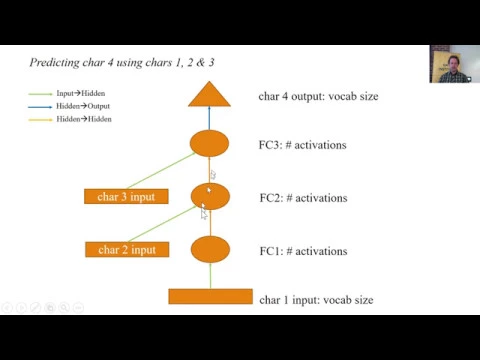
Let's go back to the standard fully connected network which looks like this. To remind you, the arrows represent one or more layer operations, generally speaking a linear, followed by a nonlinear function. In this case, they're matrix modifications, followed by ReLU or THAN. The arrows of the same color represent exactly the same weight matrix being used.

And so one thing which was just slightly different from previous fully connected networks we've seen is that we have an input coming in not just at the first layer but also at the second layer and also at the third layer. And we tried a couple of approaches, one was concatenating the inputs and one was adding the inputs.

But there was nothing at all conceptually different about this. So that code looked like this. We had a model where we basically defined the three arrows colors we had as three different weight matrices. And by using the linear class, we got actually both the weight matrix and the bias vector wrapped up for free for us.

And then we went through and we did each of our embeddings, put it through our first linear layer and then we did each of our, we call them hidden, I think they were orange arrows. And in order to avoid the fact that there's no orange arrow coming into the first one, we decided to invent an empty matrix and that way every one of these rows looked the same.

And so then we did exactly the same thing except we used a loop just to refactor the code. So it was just a code refactoring, there was no change of anything conceptually. And since we were doing a refactoring, we took advantage of that to increase the number of characters to 8 because I was too lazy to type 8 linear layers, but I'm quite happy to change the loop index to 8.

So this now loops through this exact same thing, but we had 8 of these rather than 3. So then we refactored that again by taking advantage of nn.rnn, which basically puts that loop together for us and keeps track of this h as it goes along for us. And so by using that we were able to replace the loop with a single call.

And so again, that's just a refactoring, doing exactly the same thing. So then we looked at something which was mainly designed to save some training time, which was previously, if we had a big piece of text, so we've got a movie review, we were basically splitting it up into 8-character segments, and we'd grab segment number 1 and use that to predict the next character.

But in order to make sure we used all of the data, we didn't just split it up like that, we actually said here's our whole thing, the first will be to grab this section, the second will be to grab that section, then that section, then that section, and each time we're predicting the next one character along.

And so I was a bit concerned that that seems pretty wasteful because as we calculate this section, nearly all of it overlaps with the previous section. So instead what we did was we said what if we actually did split it into non-overlapping pieces and we said let's grab this section here and use it to predict every one of the characters one along.

And then let's grab this section here and use it to predict every one of the characters one along. So after we look at the first character in, we try to predict the second character. And then after we look at the second character, we try to predict the third character.

And then what if you perceptive folks asked a really interesting question, or expressed a concern, which was, after we got through the first point here, we kind of threw away our H activations and started a new one, which meant that when it was trying to use character 1 to predict character 2, it's got nothing to go on.

It's only done one linear layer, and so that seems like a problem, which indeed it is. So we're going to do the obvious thing, which is let's not throw away H. So let's not throw away that matrix at all. So in code, the big problem is here. Every time we call forward, in other words every time we do a new mini-batch, we're creating our hidden state, which remember is the orange circles, we're resetting it back to a bunch of zeroes.

And so as we go to the next non-overlapping section, we're saying forget everything that's come before. But in fact, the whole point is we know exactly where we are, we're at the end of the previous section and about to start the next contiguous section, so let's not throw it away.

So instead the idea would be to cut this out, move it up to here, store it away in self, and then kind of keep updating it. So we're going to do that, and there's going to be some minor details to get right. So let's start by looking at the model.

So here's the model, it's nearly identical, but I've got, as expected, one more line in my constructor where I call something called init_hidden, and as expected init_hidden sets self.h to be a bunch of zeroes. So that's entirely unsurprising. And then as you can see our RNN now takes in self.h, and it, as before, spits out our new hidden activations.

And so now the trick is to now store that away inside self.h. And so here's wrinkle number 1. If you think about it, if I was to simply do it like that, and now I train this on a document that's a million characters long, then the size of this unrolled RNN is the one that has a million circles in.

And so that's fine going forwards, but when I finally get to the end and I say here's my character, and actually remember we're doing multi-output now, so multi-output looks like this. Or if we were to draw the unrolled version of multi-output, we would have a triangle coming off at every point.

So the problem is then when we do backpropagation, we're calculating how much does the error at character 1 impact the final answer, how much does the error at character 2 impact the final answer, and so forth. And so we need to go back through and say how do we have to update our weights based on all of those errors.

And so if there are a million characters, my unrolled RNN is a million layers long, I have a 1 million layer fully connected network. And I didn't have to write the million layers because I have the for loop and the for loop is hidden away behind the self dot RNN, but it's still there.

So this is actually a 1 million layer fully connected network. And so the problem with that is it's going to be very memory intensive because in order to do the chain rule, I have to be able to multiply it every step like f'u g'x. So I have to remember those values u, the value of every set of layers, so I'm going to have to remember all those million layers, and I'm going to have to do a million multiplications, and I'm going to have to do that every batch.

So that would be bad. So to avoid that, we basically say from time to time, I want you to forget your history. So we can still remember the state, which is to remember what's the actual values in our hidden matrix, but we can remember the state without remembering everything about how we got there.

So there's a little function called repackaged variable, which literally is just this. It just simply says, grab the tensor out of it, because remember the tensor itself doesn't have any concept of history, and create a new variable out of that. And so this variable is going to have the same value, but no history of operations, and therefore when it tries to backpropagate, it'll stop there.

So basically what we're going to do then is we're going to call this in our forward. So that means it's going to do 8 characters, it's going to backpropagate through 8 layers, it's going to keep track of the actual values in our hidden state, but it's going to throw away at the end of those 8 its history of operations.

So this approach is called backprop through time, and when you read about it online, people make it sound like a different algorithm, or some big insight or something, but it's not at all. It's just saying hey, after our for loop, just throw away your history of operations and start afresh.

So we're keeping our hidden state, but we're not keeping our hidden state's history. So that's wrinkle number 1, that's what this repackage bar is doing. So when you see bptt, that's referring to backprop through time, and you might remember we saw that in our original RNN lesson, we had a variable called bptt = 70, and so when we set that, we're actually saying how many layers to backprop through.

Another good reason not to backprop through too many layers is if you have any kind of gradient instability like gradient explosion or gradient spanishing, the more layers you have, the harder the network gets to train. So it's slower and less resilient. On the other hand, a longer value for bptt means that you're able to explicitly capture a longer kind of memory, more state.

So that's something that you get to tune when you create your RNN. Wrinkle number 2 is how are we going to put the data into this. It's all very well the way I described it just now where we said we could do this, and we can first of all look at this section, then this section, then this section, but we want to do a mini-batch at a time, we want to do a bunch at a time.

So in other words, we want to say let's do it like this. So mini-batch number 1 would say let's look at this section and predict that section. And at the same time in parallel, let's look at this totally different section and predict this. And at the same time in parallel, let's look at this totally different section and predict this.

And so then, because remember in our hidden state, we have a vector of hidden state for everything in our mini-batch, so it's going to keep track of at the end of this is going to be a vector here, a vector here, a vector here, and then we can move across to the next one and say okay, for this part of the mini-batch, use this to predict that, and use this to predict that, and use this to predict that.

So you can see that we've got a number of totally separate bits of our text that we're moving through in parallel. So hopefully this is going to ring a few bells for you, because what happened was back when we started looking at TorchText for the first time, we started talking about how it creates these mini-batches.

And I said what happened was we took our whole big long document consisting of the entire works of Nietzsche, or all of the IMDb reviews concatenated together, or whatever, and a lot of you, not surprisingly, because this is really weird at first, a lot of you didn't quite hear what I said correctly.

What I said was we split this into 64 equal-sized chunks, and a lot of your brains went, "Jermi just said we split this into chunks of size 64." But that's not what Jermi said. Jermi said we split it into 64 equal-sized chunks. So if this whole thing was length 64 million, which would be a reasonable sized corpus, then each of our 64 chunks would have been of length 1 million.

And so then what we did was we took the first chunk of 1 million and we put it here. And then we took the second chunk of 1 million and we put it here. The third chunk of 1 million, we put it here. And so forth to create 64 chunks.

And then each mini-batch consisted of us going, "Let's split this down here, and here, and here." And each of these is of size BPTT, which I think we had something like 70. And so what happened was we said, "All right, let's look at our first mini-batch is all of these." So we do all of those at once and predict everything offset by 1.

And then at the end of that first mini-batch, we went to the second chunk and used each one of these to predict the next one offset by 1. So that's why we did that slightly weird thing, is that we wanted to have a bunch of things we can look through in parallel, each of which hopefully are far enough away from each other that we don't have to worry about the fact that the truth is the start of this million characters was actually in the middle of a sentence, but who cares?

Because it only happens once every million characters. I was wondering if you could talk a little bit more about augmentation for this kind of dataset? Data augmentation for this kind of dataset? Yeah. No, I can't because I don't really know a good way. It's one of the things I'm going to be studying between now and Part 2.

There have been some recent developments, particularly something we talked about in the machine learning course, which I think we briefly mentioned here, which was somebody for a recent Kaggle competition won it by doing data augmentation by randomly inserting parts of different rows, basically. Something like that may be useful here, and I've seen some papers that do something like that, but I haven't seen any kind of recent-ish state-of-the-art NLP papers that are doing this kind of data augmentation, so it's something we're planning to work on.

So Jeremy, how do you choose BPTT? So there's a couple of things to think about when you pick your BPTT. The first is that you'll note that the matrix size for a mini-batch has BPTT by batch size. So one issue is your GPU RAM needs to be able to fit that by your embedding matrix, because every one of these is going to be of length embedding, plus all of the hidden state.

So one thing is if you get a CUDA out of memory error, you need to reduce one of those. If your training is very unstable, like your loss is shooting off to NAN suddenly, then you could try decreasing your BPTT because you've got less layers to gradient explode through.

You could try decreasing your BPTT because it's got to do one of those steps at a time, like that for loop can't be paralyzed. Well I say that. There's a recent thing called QRNN, which we'll hopefully talk about in Part 2 which kind of does paralyze it, but the versions we're looking at don't paralyze it.

So that would be the main issues, look at performance, look at memory, and look at stability, and try and find a number that's as high as you can make it, but all of those things work for you. So trying to get all that chunking and lining up to work is more code than I want to write, so for this section we're going to go back and use Torch Text again.

When you're using APIs like FastAI and Torch Text, which in this case these two APIs are designed to work together, you often have a choice which is like, okay, this API has a number of methods that expect the data in this kind of format, and you can either change your data to fit that format, or you can write your own data set subclass to handle the format that your data is already in.

I've noticed on the forum a lot of you are spending a lot of time writing your own data set classes, whereas I am way lazier than you and I spend my time instead changing my data to fit the data set classes I have. Either is fine, and if you realize there's a kind of a format of data that me and other people are likely to be seeing quite often and it's not in the FastAI library, then by all means write the data set subclass, submit it as a PR, and then everybody can benefit.

In this case, I just thought I want to have some niche data fed into Torch Text, I'm just going to put it in the format that Torch Text kind of already supports. So Torch Text already has, or at least the FastAI wrapper around Torch Text, already has something where you can have a training path and a validation path and one or more text files in each path containing a bunch of stuff that's concatenated together for your language model.

So in this case, all I did was I made a copy of my nature file, copied it into training, made another copy, stuck it into the validation, and then in the training set, I deleted the last 20% of rows, and in the validation set, I deleted all except for the last 20% of rows.

And I was done. In this case, I found that easier than writing a custom data set class. The other benefit of doing it that way was that I felt like it was more realistic to have a validation set that wasn't a random shuffled set of rows of text, but was like a totally separate part of the corpus, because I feel like in practice you're very often going to be saying, "Oh, I've got these books or these authors I'm learning from, and then I want to apply it to these different books and these different authors." So I felt like getting a more realistic validation of my nature model, I should use a whole separate piece of the text, so in this case it was the last 20% of the rows of the corpus.

So I haven't created this for you intentionally, because this is the kind of stuff I want you practicing is making sure that you're familiar enough, comfortable enough with bash or whatever you can create these, and that you understand what they need to look like and so forth. So in this case, you can see I've now got a train and a validation here, and then I could go inside here.

So you can see I've literally just got one file in it, because when you're doing a language model, i.e. predicting the next character or predicting the next word, you don't really need separate files. It's fine if you do have separate files, but they just get concatenated together anyway. So that's my source data, and so here is the same lines of code that we've seen before, and let's go over them again because it's a couple of lessons ago.

So in Torch Text, we create this thing called a field, and a field initially is just a description of how to go about pre-processing the text. In this case, I'm going to say lowercase it, because I don't -- now I think about it, there's no particular reason to have done this lowercase, uppercase would work fine too.

And then how do I tokenize it? And so you might remember last time we used a tokenization function which largely spit on white space and tried to do clever things with punctuation, and that gave us the word model. In this case, I want a character model, so I actually want every character put into a separate token.

So I can just use the function list in Python, because list in Python does that. So this is where you can kind of see like, understanding how libraries like Torch Text and FastAI are designed to be extended can make your life a lot easier. So when you realize that very often, both of these libraries kind of expect you to pass a function that does something, and then you realize, oh, I can write any function I like.

So this is now going to mean that each mini-batch is going to contain a list of characters. And so here's where we get to define all our different parameters. And so to make it the same as previous sections of this notebook, I'm going to use the same batch size, the same number of characters, and I'm going to rename it to bptt since we know what that means.

The number of the size of the embedding, and the size of our hidden state. Remembering the size of our hidden state simply means going all the way back to the start, and then hidden simply means the size of the state that's created by each of those orange arrows. So it's the size of each of those circles.

So having done that, we can then create a little dictionary saying what's our training, validation and test set. In this case, I don't have a separate test set, so I'll just use the same thing. And then I can say I want a language model data subclass with model data, I'm going to grab it from text files, and this is my path, and this is my field, which I defined earlier, and these are my files, and these are my hyperparameters.

MinFract is not going to do anything actually in this case because I don't think there's going to be any character that appears less than 3 times, so that's probably redundant. So at the end of that, it says there's going to be 963 batches to go through. And so if you think about it, that should be equal to the number of tokens divided by the batch size divided by bptt, because that's the size of each of those rectangles.

You'll find that in practice it's not exactly that, and the reason it's not exactly that is that the authors of TorchText did something pretty smart, which I think we've briefly mentioned this before. They said we can't shuffle the data, like with images we like to shuffle the order so every time we see them in a different order, so there's a bit more randomness.

We can't shuffle because we need to be contiguous, but what we could do is basically randomize bptt a little bit each time. And so that's what PyTorch does. It's not always going to give us exactly 8 characters long, 5% of the time it'll actually cut it in half, and then it's going to add on a small little standard deviation to make it slightly bigger or smaller than 4 or 8.

So it's going to be slightly different to 8 on average. So a mini-batch needs to do a matrix multiplication, and the mini-batch size has to remain constant because we've got this h-weight matrix that has to line up in size with the size of the mini-batch. But the sequence length can change, no problem.

So that's why we have 963, so the length of a data loader is how many mini-batches, in this case it's a little bit approximate. Number of tokens is how many unique things are in the vocabulary. And remember, after we run this line, text now does not just contain a description of what we want, but it also contains an extra attribute called vocab, which contains stuff like a list of all of the unique items in the vocabulary and a reverse mapping from each item to its number.

So that text object is now an important thing to keep track of. Let's now try this. Now we started out by looking at the class. So the class is exactly the same as the class we've had before. The only key difference is to call init_hidden, which sets out. So h is not a variable anymore, it's now an attribute, self.h is a variable containing a bunch of zeroes.

Now I mentioned that batch size remains constant each time, but unfortunately when I said that I lied to you. And the way that I lied to you is that the very last mini-batch will be shorter. The very last mini-batch is actually going to have less than 64 -- it might be exactly the right size if it so happens that this data set is exactly divisible by bptt times batch size.

But it probably isn't, so the last batch will probably have a little bit less. And so that's why I do a little check here that says let's check that the batch size inside self.h is going to be the height, the number of activations, and the width is going to be the mini-batch size.

Check that that's equal to the actual batch size length that we've received. And if they're not the same, then set it back to zeroes again. So this is just a minor little ring call that basically at the end of each epoch, it's going to do like a little mini-batch.

And so then as soon as it starts the next epoch, it's going to see that they're not the same again, and it will reinitialize it to the correct full batch size. So that's why if you're wondering, there's an init hidden not just in the constructor, but also inside forward, it's to handle this end of each epoch, start of each epoch difference.

Not an important point by any means, but potentially confusing when you see it. So the last ring call. The last ring call is something that slightly sucks about PyTorch, and maybe somebody can be nice enough to try and fix it with a PR if anybody feels like it, which is that the loss functions such as softmax are not happy receiving a rank 3 tensor.

Remember a rank 3 tensor is just another way of saying a dimension 3 array. There's no particular reason they ought to not be happy receiving a rank 3 tensor. Like somebody could write some code to say hey, a rank 3 tensor is probably a sequence length by batch size by results thing, and so you should just do it for each of the two initial axes.

But no one's done that. And so it expects it to be a rank 2 tensor. Funnily enough, it can handle rank 2 or rank 4, but not rank 3. So we've got a rank 2 tensor containing, for each time period (I can't remember which way around the axes are, but whatever) for each time period for each batch, we've got our predictions.

And then we've got our actuals for each time period for each batch, we've got our predictions, and we've got our actuals. And so we just want to check whether they're the same. And so in an ideal world, our loss function would check item 1 1, then item 1 2, and then item 1 3, but since that hasn't been written, we just have to flatten them both out.

We can literally just flatten them out, put rows to rows. And so that's why here I have to use .view, and so .view says the number of columns will be equal to the size of the vocab, because remember we're going to end up with a probability for each letter.

And then the number of rows is however big is necessary, which will be equal to batch size times bptt. And then you may be wondering where I do that for the target, and the answer is torch text knows that the target needs to look like that, so torch text has already done that for us.

So torch text automatically changes the target to be flattened out. And you might actually remember if you go back to lesson 4 when we actually looked at a mini-batch that spat out of torch text, we noticed actually that it was flattened, and I said we'll learn about why later, and so later is now arrived.

So there are the 3 wrinkles. Get rid of the history, I guess 4 wrinkles. Recreate the hidden state if the batch size changes, flatten out, and then use torch text to create mini-batches that line up nicely. So once we do those things, we can then create our model, create our optimizer with that model's parameters, and fit it.

One thing to be careful of here is that softmax now, as of PyTorch 0.3, requires that we pass in a number here saying which axis do we want to do the softmax over. So at this point, this is a 3-dimensional tensor, and so we want to do the softmax over the final axis.

So when I say which axis do we do the softmax over, remember we divide by, so we go e to the x_i divided by the sum of e to the x_i. So it's saying which axis do we sum over, so which axis do we want to sum to 1.

And so in this case, clearly we want to do it over the last axis, because the last axis is the one that contains the probability per letter of the alphabet, and we want all of those probabilities to sum to 1. So therefore, to run this notebook, you're going to need PyTorch 0.3, which just came out this week.

So if you're doing this on the MOOC, you're fine, I'm sure you've got at least 0.3 or later. Where else are the students here? The really great news is that 0.3, although it does not yet officially support Windows, it does in practice. I successfully installed 0.3 from Conda yesterday by typing Conda install PyTorch in Windows.

I then attempted to use the entirety of Lesson 1, and every single part worked. So I actually ran it on this very laptop. So for those who are interested in doing deep learning on their laptop, I can definitely recommend the New Surface Book. The New Surface Book 15" has a GTX 1060 6GB GPU in it, and it was running about 3 times slower than my 1080Ti, which I think means it's about the same speed as an AWS P2 instance.

And as you can see, it's also a nice convertible tablet that you can write on, and it's thin and light, so I've never seen such a good deep learning box. Also I successfully installed Linux on it, and all of the fastai stuff worked on the Linux as well, so a really good option if you're interested in a laptop that can run deep learning stuff.

So that's going to be aware of with this dm= -1. So then we can go ahead and construct this, and we can call fit, and we're basically going to get pretty similar results to what we got before. So then we can go a bit further with our RNN by just unpacking it a bit more.

And so this is now exactly the same thing, gives exactly the same answers, but I have removed the call to RNN. So I've got rid of this self.RNN. And so this is just something, I won't spend time on it, but you can check it out. So instead, I've now defined RNN as RNN cell, and I've copied and pasted the code above.

Don't run it, this is just for your reference, from PyTorch. This is the definition of RNN cell in PyTorch. And I want you to see that you can now read PyTorch source code and understand it. Not only that, you'll recognize it as something we've done before. It's a matrix multiplication of the weights by the inputs plus biases.

So f.linear simply does a matrix product followed by an addition. And interestingly, you'll see they do not concatenate the input bit and the hidden bit, they sum them together, which is our first approach. As I said, you can do either, neither one is right or wrong, but it's interesting to see that this is the definition here.

Can you give us an insight about what are they using that particular activation function? I think we might have briefly covered this last week, but very happy to do it again if I did. Basically, than looks like that. So in other words, it's a sigmoid function, double the height -1, literally, they're equal.

So it's a nice function in that it's forcing it to be no smaller than -1, no bigger than +1. And since we're multiplying by this weight matrix again and again and again and again, we might worry that a ReLU, because it's unbounded, might have more of a gradient explosion problem.

That's basically the theory. Having said that, you can actually ask PyTorch for an RNN cell which uses a different nonlinearity. So you can see by default it uses than, but you can ask for a ReLU as well. But most people seem to, pretty much everybody still seems to use than as far as I can tell.

So you can basically see here, this is all the same except now I've got an RNN cell, which means now I need to put my for loop back. And you can see every time I call my little linear function, I just append the result onto my list. And at the end, the result is that all stacked up together.

So I'm just trying to show you how nothing inside PyTorch is mysterious, you should find you get basically exactly the same answer from this as the previous one. In practice you would never write it like this, but what you may well find in practice is that somebody will come up with a new kind of RNN cell, or a different way of keeping track of things over time, or a different way of doing regularization.

And so inside fastai's code, you will find that we do this by hand because we use some regularization approaches that aren't supported by PyTorch. So another thing I'm not going to spend much time on but I'll mention briefly is that nobody really uses this RNN cell in practice. And the reason we don't use that RNN cell in practice is even though the than is here, you do tend to find gradient explosions are still a problem, so we have to use pretty low learning rates to get these to train, and pretty small values for bptt to get them to train.

So what we do instead is we replace the RNN cell with something like this. This is called a GRU cell, and here's a picture of it, and there's the equations for it. So basically I'll show you both quickly, but we'll talk about it much more in Part 2. We've got our input, and our input normally gets multiplied by a weight matrix to create our new activations.

That's not what happens, and then of course we add it to the existing activations. That's not what happens here. In this case, our input goes into this h_tilde temporary thing, and it doesn't just get added to our previous activations, but our previous activations get multiplied by this value R.

And R stands for reset, it's a reset gate. And how do we calculate this value, it goes between 0 and 1 in our reset gate? Well the answer is, it's simply equal to a matrix product between some weight matrix and the concatenation of our previous hidden state and our new input.

In other words, this is a little one hidden layer neural net. And in particular it's a one hidden layer neural net because we then put it through the sigmoid function. One of the things I hate about mathematical notation is symbols are overloaded a lot. When you see sigma, that means standard deviation.

When you see it next to a parenthesis like this, it means the sigmoid function. So in other words, that which looks like that. So this is like a little mini-neuronet with no hidden layers, so to think of it another way is like a little logistic regression. And I mentioned this briefly because it's going to come up a lot in part 2, so it's a good thing to start learning about.

It's this idea that in the very learning itself, you can have little mini-neuronets inside your neural nets. And so this little mini-neuronet is going to be used to decide how much of my hidden state am I going to remember. And so it might learn that in this particular situation, forget everything you know.

For example, there's a full stop. When you see a full stop, you should throw away nearly all of your hidden state. That is probably something it would learn, and that's very easy for it to learn using this little mini-neuronet. And so that goes through to create my new hidden state along with the input.

And then there's a second thing that happens, which is there's this gate here called z. And what z says is you've got some amount of your previous hidden state plus your new input, and it's going to go through to create your new state. And I'm going to let you decide to what degree do you use this new input version of your hidden state, and to what degree will you just leave the hidden state the same as before.

So this thing here is called the update gate. And so it's got two choices it can make. The first is to throw away some hidden state when deciding how much to incorporate that versus my new input, and how much to update my hidden state versus just leave it exactly the same.

And the equation hopefully is going to look pretty familiar to you, which is check this out here. Remember how I said you want to start to recognize some common ways of looking at things? Well here I have a 1 minus something by a thing, and a something without the 1 minus by a thing, which remember is a linear interpolation.

So in other words, the value of z is going to decide to what degree do I have keep the previous hidden state, and to what degree do I use the new hidden state. So that's why they draw it here as this kind of like, it's not actually a switch, but you can put it in any position.

You can be like, oh it's here, or it's here, or it's here to decide how much to update. So they're basically the equations. It's a little mini-neuronet with its own weight matrix to decide how much to update, a little mini-neuronet with its own weight matrix to decide how much to reset, and then that's used to do an interpolation between the two hidden states.

So that's called a GRU, gated recurrent network. There's the definition from the PyTorch source code. They have some slight optimizations here that if you're interested in we can talk about them on the forum, but it's exactly the same formula we just saw. And so if you go nn.giu, then it uses this same code, but it replaces the RNN cell with this cell.

And as a result, rather than having something where we're getting a 1.54, we're now getting down to 1.40, and we can keep training even more, get right down to 1.36. So in practice, a GRU, or very nearly equivalently, we'll see in a moment, an LSTM, is in practice what pretty much everybody always uses.

So the RT and HT are ultimately scalars after they go through the sigmoid, but they're applied element-wise. Is that correct? Yes, although of course one for each mini-batch. On the excellent Chris Olar's blog, there's an understanding LSTM networks post, which you can read all about this in much more detail if you're interested.

And also, the other one I was dealing with here is WildML, I also have a good blog post on this. If somebody wants to be helpful, feel free to put them in the lesson wiki. So then putting it all together, I'm now going to replace my GRU with an LSTM.

I'm not going to bother showing you the cell for this, it's very similar to GRU. But the LSTM has one more piece of state in it called the cell state, not just the hidden state. So if you do use an LSTM, you now inside your init_hidden have to return a tuple of matrices.

They're exactly the same size as the hidden state, but you just have to return the tuple. The details don't matter too much, but we can talk about it during the week if you're interested. When you pass in, you still pass in self.h, it still returns a new value of h, you still can repackage it in the usual way.

So this code is identical to the code before. One thing I've done though is I've added dropout inside my RNN, which you can do with the PyTorch RNN function, so that's going to do dropout after each time step. And I've doubled the size of my hidden layer since I've now added 0.5 dropout, and so my hope was that this would be able to learn more but be more resilient as it does so.

So then I wanted to show you how to take advantage of a little bit more fast.ai magic without using the layer class. And so I'm going to show you how to use callbacks, and specifically we're going to do SGDR without using the learner class. So to do that, we create our model again, just a standard PyTorch model.

And this time, rather than going, remember the usual PyTorch approach is opt=optim.atom and you pass in the parameters and the learning rate, I'm not going to do that, I'm going to use the fast.ai layer optimizer class, which takes my optim class constructor from PyTorch. It takes my model, it takes my learning rate, and optionally takes weight decay.

And so this class is tiny, it doesn't do very much at all. The key reason it exists is to do differential learning rates and differential weight decay. But the reason we need to use it is that all of the mechanics inside fast.ai assumes that you have one of these.

So if you want to use callbacks or SGDR or whatever in code where you're not using the learner class, then you need to use, rather than saying opt=optim.atom, and here's my parameters, you instead say layer optimizer. So that gives us a layer optimizer object, and if you're interested, basically behind the scenes, you can now grab a .opt property which actually gives you the optimizer.

You don't have to worry about that yourself, but that's basically what happens behind the scenes. The key thing we can now do is that when we call fit, we can pass in that optimizer, and we can also pass in some callbacks. And specifically we're going to use the cosine annealing callback.

And so the cosine annealing callback requires a layer optimizer object. And so what this is going to do is it's going to do cosine annealing by changing the learning rate inside this object. So the details are terribly important, we can talk about them on the forum, it's really the concept I wanted to get across here.

Which is that now that we've done this, we can say create a cosine annealing callback which is going to update the learning rates in this layer optimizer. The length of an epoch is equal to this here. How many mini batches are there in an epoch? Well it's whatever the length of this data loader is, because it's going to be doing the cosine annealing, it needs to know how often to reset.

And then you can pass in the cycle melt in the usual way. And then we can even save our model automatically, like remember how there was that cycle save name parameter that we can pass to learn.fit? This is what it does behind the scenes. It sets an on-cycle end callback, and so here I have to find that callback as being something that saves my model.

So there's quite a lot of cool stuff that you can do with callbacks. Callbacks are basically things where you can define at the start of training, or at the start of an epoch, or at the start of a batch, or at the end of training, or at the end of an epoch, or at the end of a batch, please call this code.

And so we've written some for you, including SGDR, which is the cosine annealing callback. And then Sahar recently wrote a new callback to implement the new approach to decoupled rate decay. We use callbacks to draw those little graphs of the loss of a time, so there's lots of cool stuff you can do with callbacks.

So in this case, by passing in that callback, we're getting SGDR, and that's able to get us down to 1.31 here, and then we can train a little bit more, and eventually get down to 1.25. And so we can now test that out. And so if we pass in a few characters of text, we get not surprisingly an e after 4 or thus.

Let's do then 400, and now we have our own Nietzsche. So Nietzsche tends to start his sections with a number and a dot. So 293, perhaps that every life of values of blood, of intercourse, when it senses there is unscrupulous, his very rights and still impulse love. So it's slightly less clear than Nietzsche normally, but it gets the tone right.

And it's actually quite interesting to play around with training these character-based language models, to run this at different levels of loss, to get a sense of what does it look like. You really notice that this is like 1.25, and at slightly worse, like 1.3, this looks like total junk.

There's punctuation in random places and nothing makes sense. And you start to realize that the difference between Nietzsche and random junk is not that far in language model terms. And so if you train this for a little bit longer, you'll suddenly find it's making more and more sense. So if you are playing around with NLP stuff, particularly generative stuff like this, and you're like, the results are kind of okay but not great, don't be disheartened because that means you're actually very very nearly there.

The difference between something which is starting to create something which almost vaguely looks English if you squint, and something that's actually a very good generation, it's not far in loss function terms. So let's take a 5-minute break, we'll come back at 7.45 and we're going to go back to computer vision.

So now we come full circle back to vision. So now we're looking at lesson 7, sci-fi 10 notebook. You might have heard of sci-fi 10. It's a really well-known dataset in academia. And it's actually pretty old by computer vision standards, well before ImageNet was around, there was sci-fi 10.

You might wonder why we're going to be looking at such an old dataset, and actually I think small datasets are much more interesting than ImageNet. Because most of the time you're likely to be working with stuff with a small number of thousands of images rather than 1.5 million images.

Some of you will work with 1.5 million images, but most of you won't. So learning how to use these kind of datasets I think is much more interesting. Often also a lot of the stuff we're looking at in medical imaging, we're looking at the specific area where there's a lung nodule, you're probably looking at 32x32 pixels at most as being the area where that lung nodule actually exists.

And so sci-fi 10 is small both in terms of it doesn't have many images, and the images are very small, and so therefore I think in a lot of ways it's much more challenging than something like ImageNet. In some ways it's much more interesting. And also, most importantly, you can run stuff much more quickly on it, so it's much better to test out your algorithms with something you can run quickly, and it's still challenging.

And so I hear a lot of researchers complain about how they can't afford to study all the different versions of their algorithm properly because it's too expensive, and they're doing it on ImageNet. So it's literally a week of expensive GPU work for every study they do, and I don't understand why you would do that kind of study on ImageNet, it doesn't make sense.

And so there's been a lot of debate about this this week because a really interesting researcher named Ali Rahami at NIPS this week gave a talk, a really great talk about the need for rigor in experiments in deep learning, and he felt like there's a lack of rigor. And I've talked to him about it quite a bit since that time, and I'm not sure we yet quite understand each other as to where we're coming from, but we have very similar kinds of concerns, which is basically people aren't doing carefully tuned, carefully thought about experiments, but instead they throw lots of GPUs and lots of data and consider that a day.

And so this idea of saying, well, is my algorithm meant to be good at small images, at small data sets, well if so, let's study it on so far 10 rather than studying it on ImageNet and then do more studies of different versions of the algorithm, turning different bits on and off, understand which parts are actually important, and so forth.

People also complain a lot about MNIST, which we've looked at before, and I would say the same thing about MNIST, which is like if you're actually trying to understand which parts of your algorithm make a difference and why, using MNIST for that kind of study is a very good idea.

And all these people who complain about MNIST, I think they're just showing off. They're saying, I work at Google and I have a pod of TPUs and I have $100,000 a week of time to spend on it, no worries. But I think that's all it is, it's just signaling rather than actually academically rigorous.

Okay, so sci-fi 10, you can download from here. This person has very kindly made it available in image form. If you Google for sci-fi 10, you'll find a much less convenient form, so please use this one. It's already in the exact form you need. Once you download it, you can use it in the usual way.

So here's a list of the classes that are there. Now you'll see here I've created this thing called stats. Normally when we've been using pre-trained models, we have been saying transforms from model, and that's actually created the necessary transforms to convert our dataset into a normalized dataset based on the means and standard deviations of each channel in the original model that was trained.

In our case, this time we've got to train a model from scratch, so we have no such thing. So we actually need to tell it the mean and standard deviation of our data to normalize it. And so in this case, I haven't included the code here to do it.

You should try and try this yourself to confirm that you can do this and understand where it comes from. But this is just the mean per channel and the standard deviation per channel of all of the images. So we're going to try and create a model from scratch. And so the first thing we need is some transformations.

So for sci-fi 10, people generally do data augmentation of simply flipping randomly horizontally. So here's how we can create a specific list of augmentations to use. And then they also tend to add a little bit of black padding around the edge and then randomly pick a 32x32 spot from within that padded image.

So if you add the pad parameter to any of the fastai transform creators, it'll do that for you. And so in this case, I'm just going to add 4 pixels around each size. And so now that I've got my transforms, I can go ahead and create my image_classifier data.from_paths in the usual way.

I'm going to use a batch size of 256 because these are pretty small, so it's going to let me do a little bit more at a time. So here's what the data looks like. So for example, here's a boat. And just to show you how tough this is, what's that?

It's a frog. So I guess it's this big thing, whatever the thing is called, there's your frog. So these are the kinds of things that we want to look at. So I'm going to start out, so our student, Karim, we saw one of his posts earlier in this course, he made this really cool notebook which shows how different optimizers work.

So Karim made this really cool notebook, I think it was maybe last week, in which he showed how to create various different optimizers from scratch. So this is kind of like the Excel thing I had, but this is the Python version of Momentum and Adam and Nesterov and Adagrad, all written from scratch, which is very cool.

One of the nice things he did was he showed a tiny little general-purpose fully connected network generator. So we're going to start with his. So he called that SimpleNet, so are we. So here's a simple class which has a list of fully connected layers. Whenever you create a list of layers in PyTorch, you have to wrap it in an nn.module list just to tell PyTorch to register these as attributes.

And so then we just go ahead and flatten the data that comes in, because it's fully connected layers, and then go through each layer and call that linear layer, do the value to it, and at the end do a softmax. So there's a really simple approach, and so we can now take that model and now I'm going to show you how to step up one level of the API higher.

Rather than calling the fit function, we're going to create a learn object, but we're going to create a learn object from a custom model. And so we can do that by saying we want a convolutional learner, we want to create it from a model and from some data, and the model is this one.

This is just a general PyTorch model, and this is a model data object of the usual kind. And that will return a learner. So this is a bit easier than what we just saw with the RNN -- we don't have to fiddle around with layer optimizers and cosine annealing callbacks and whatever.

This is now a learner that we can do all the usual stuff with, but we can do it with any model that we create. So if we just go Learn, that will go ahead and print it out. You can see we've got 3,072 features coming in because we've got 32 by 32 pixels by 3 channels.

And then we've got 40 features coming out of the first layer, that's going to go into the second layer, 10 features coming out because we've got the sci-fi 10 categories. You can call dot summary to see that in a little bit more detail. We can do LRfind, we can plot that, and we can then go fit, and we can use cycle length, and so forth.

So with a simple -- how many hidden layers do we have? One hidden layer, one output layer, one hidden layer model. And here we can see the number of parameters we have is over 120,000. We get a 47% accuracy. So not great, so let's kind of try and improve it.

And so the goal here is we're going to try and eventually replicate the basic architecture of a ResNet. So that's where we're going to try and get to here, to gradually build up to a ResNet. So the first step is to replace our fully connected model with a convolutional model.

So to remind you, a fully connected layer is simply doing a dot product. So if we had all of these data points and all of these weights, then we basically do some product of all of those together, in other words it's a matrix model. And that's a fully connected layer.

And so the weight matrix is going to contain every element of the input for every element of the output. So that's why we have here a pretty big weight matrix. And so that's why despite the fact that we have such a crappy accuracy, we have a lot of parameters because in this very first layer we've got 3072 coming in and 40 coming out, so that gives us 3000x40 parameters.

And so we end up not using them very efficiently because we're basically saying every single pixel in the input has a different weight. And of course what we really want to do is find groups of 3x3 pixels that have particular patterns to them, and remember we call that a convolution.

So a convolution looks like so. We have a little 3x3 section of our image and a corresponding 3x3 set of filters, or a filter with a 3x3 kernel, and we just do a sum product of just that 3x3 by that 3x3. And then we do that for every single part of our image.

And so when we do that across the whole image, that's called a convolution. And remember, in this case we actually had multiple filters, so the result of that convolution actually had a tensor with an additional third dimension to it effectively. So let's take exactly the same code that we had before, but we're going to replace nn.linear with nn.com2d.

Now what I want to do in this case is each time I have a layer, I want to make the next layer smaller. And so the way I did that in my Excel example was I used max_pooling. So max_pooling took every 2x2 section and replaced it with its maximum value.

Nowadays we don't use that kind of max_pooling much at all. Instead nowadays what we tend to do is do what's called a Stride 2 convolution. A Stride 2 convolution, rather than saying let's go through every single 3x3, it says let's go through every second 3x3. So rather than moving this 3x3 1 to the right, we move it 2 to the right.

And then when we get to the end of the row, rather than moving one row down, we move two rows down. So that's called a Stride 2 convolution. And so a Stride 2 convolution has the same kind of effect as a max_pooling, which is you end up halving the resolution in each dimension.

So we can ask for that by saying Stride = 2. We can say we want it to be 3x3 by saying kernel size, and then the first two parameters are exactly the same as nn.linear, they're the number of features coming in and the number of features coming out. So we create a module list of those layers, and then at the very end of that, so in this case I'm going to say I've got three channels coming in, the first one layer will come out with 20, then 40, and then 80.

So if we look at the summary, we're going to start with a 32x32, we're going to spit out a 15x15, and then a 7x7, and then a 3x3. And so what do we do now to get that down to a prediction of one of 10 classes? What we do is we do something called adaptive max_pooling, and this is what is pretty standard now for state-of-the-art algorithms, is that the very last layer we do a max_pool, but rather than doing a 2x2 max_pool, we say it doesn't have to be 2x2, it could have been 3x3, which is like replace every 3x3 pixels with its maximum, it could have been 4x4.

Adaptive max_pool is where you say, I'm not going to tell you how big an area to pool, but instead I'm going to tell you how big a resolution to create. So if I said, for example, I think my input here is 28x28, if I said do a 14x14 adaptive max_pool, that would be the same as a 2x2 max_pool, because in other words it's saying please create a 14x14 output.

If I said do a 2x2 adaptive max_pool, then that would be the same as saying do a 14x14 max_pool. And so what we pretty much always do in modern CNNs is we make our penultimate layer a 1x1 adaptive max_pool. So in other words, find the single largest cell and use that as our new activation.

And so once we've got that, we've now got a 1x1 tensor, or actually 1x1 by number of features tensor. So we can then on top of that go x.view, x.size, -1, and actually there are no other dimensions to this basically. So this is going to return a matrix of mini-batch by number of features.

And so then we can feed that into a linear layer with however many classes we need. So you can see here the last thing I pass in is how many classes am I trying to predict, and that's what's going to be used to create that last layer. So it goes through every convolutional layer, does a convolution, does a ReLU, does an adaptive max_pool.

This dot view just gets rid of those trailing unit axes, the 1,1 axis, which is not necessary. That allows us to feed that into our final linear layer that bits out something of size C, which here is 10. So you can now see how it works. It goes 32 to 15 to 7x7 to 3x3.

The adaptive max_pool makes it 80 by 1 by 1, and then our dot view makes it just mini-batch size by 80, and then finally a linear layer which takes it from 80 to 10, which is what we wanted. So that's our most basic -- you'd call this a fully convolutional network, so a fully convolutional network is something where every layer is convolutional except for the very last.

So again, we can now go lr.find, and now in this case when I did lr.find, it went through the entire data set and was still getting better. And so in other words, the default final learning rate it tries is 10, and even at that point it was still pretty much getting better.

So you can always override the final learning rate by saying end_lr=, and that'll just get it to try more things. So here is the learning rate finder, and so I picked 10^-1, trained that for a while, and that's looking pretty good, so then I tried it with a cycle length of 1, and it's starting to flatten out at about 60%.

So you can see here the number of parameters I have here are 500, 7000, 28000, about 30,000. So I have about 1/4 of the number of parameters, but my accuracy has gone up from 47% to 60%. And the time per epoch here is under 30 seconds, and here also.

So the time per epoch is about the same. And that's not surprising because when you use small simple architectures, most of the time is the memory transfer, the actual time during the compute is trivial. So I'm going to refactor this slightly because I want to try and put less stuff inside my forward, and so calling relu every time doesn't seem ideal.

So I'm going to create a new class called conv_layer, and the conv_layer class is going to contain a convolution with a kernel size of 3 and a stride of 2. One thing I'm going to do now is add padding. Did you notice here the first layer went from 32x32 to 15x15, not 16x16?

And the reason for that is that at the very edge of your convolution, here, see how this first convolution, there isn't a convolution where the middle is the top left point because there's nothing outside it. Or else if we had put a row of 0's at the top and a row of 0's at the edge of each column, we now could go all the way to the edge.

So pad=1 adds that little layer of 0's around the edge for us. And so this way we're going to make sure that we go 32x32 to 16x16 to 8x8. It doesn't matter too much when you've got these bigger layers, but by the time you get down to 4x4, you really don't want to throw away a whole piece.

So padding becomes important. So by refactoring it to put this with its defaults here, and then in the forward I'll put the ReLU in here as well, it makes my ConvNet a little bit smaller and more to the point it's going to be easier for me to make sure that everything's correct in the future by always using this ConvLayer class.

So now you know not only how to create your own neural network model, but how to create your own neural network layer. So here now I can use ConvLayer. This is such a cool thing about PyTorch is a layer definition and a neural network definition are literally identical. They both have a constructor and a forward.

And so anytime you've got a layer, you can use it as a neural net, anytime you have a neural net, you can use it as a layer. So this is now the exact same thing as we had before. One difference is I now have padding. And another thing just to show you, you can do things differently.

Back here, my max_pull I did as an object, I used the class nn.adaptive_max_pull, and I stuck it in this attribute and then I called it. But this actually doesn't have any state. There's no weights inside max_pulling, so I can actually do it with a little bit less code by calling it as a function.

So everything that you can do as a class, you can also do as a function inside this capital F which is nn.functional. So this should be a tiny bit better because this time I've got the padding. I didn't train it for as long to actually check, so let's skip over that.

So one issue here is that in the end, when I tried to add more layers, I had trouble training it. The reason I was having trouble training it was if I used larger learning rates, it would go off to nin, and if I used smaller learning rates, it kind of takes forever and doesn't really have a chance to explore properly.

So it wasn't resilient. So to make my model more resilient, I'm going to use something called batch normalization, which literally everybody calls batchnorm. And batchnorm is a couple of years old now, and it's been pretty transformative since it came along because it suddenly makes it really easy to train deeper networks.

So the network I'm going to create is going to have more layers. I've got 1, 2, 3, 4, 5 convolutional layers plus a fully connected layer. So back in the old days, that would be considered a pretty deep network and we'd be considered pretty hard to train. Nowadays it's super simple thanks to batchnorm.

Now to use batchnorm, you can just write in nn.batchnorm, but to learn about it, we're going to write it from scratch. So the basic idea of batchnorm is that we've got some vector of activations. Any time I draw a vector of activations, obviously I mean you can repeat it for the minibatch, so pretend it's a minibatch of 1.

So we've got some vector of activations, and it's coming into some layer, so probably some convolutional matrix multiplication, and then something comes out the other side. So imagine this is just a matrix multiply, say it was an identity matrix. Then every time I multiply it by that across lots and lots of layers, my activations are not getting bigger, they're not getting smaller, they're not changing at all.

That's all fine, but imagine if it was actually like 2, 2, 2. And so if every one of my weight matrices or filters was like that, then my activations are doubling each time. And so suddenly I've got this exponential growth, and in deep models that's going to be a disaster because my gradients are exploding at an exponential rate.

And so the challenge you have is that it's very unlikely unless you try carefully to deal with it that your weight matrices on average are not going to cause your activations to keep getting smaller and smaller, or keep getting bigger and bigger. You have to carefully control things to make sure that they stay at a reasonable size, you want to keep them at a reasonable scale.

So we start things off with 0 mean standard deviation 1 by normalizing the inputs, but what we'd really like to do is to normalize every layer, not just the inputs. And so, okay, fine, let's do that. So here I've created a bn layer which is exactly like my conv layer.

It's got my conv2d with my stride, my padding. I do my conv and my relu, and then I calculate the mean of each channel or of each filter, and the standard deviation of each channel or each filter, and then I subtract the means and divide by the standard deviations.

So now I don't actually need to normalize my input at all because it's actually going to do it automatically. It's normalizing it per channel, and for later layers it's normalizing it per filter. So it turns out that's not enough because SGD is bloody-minded. And so if SGD decided that it wants the weight matrix to be like so, where that matrix is something which is going to increase the values overall repeatedly, then subtract the means and divide by the standard deviations just means the next mini-batch is going to try and do it again.

So it turns out that this actually doesn't help, it literally does nothing because SGD is just going to go ahead and undo the next mini-batch. So what we do is we create a new multiplier for each channel and a new added value for each channel, and we just start them out as the addition is just a bunch of zeros, so for the first layer, 3 zeros, and the multiplier for the first layer is just 3 ones.

So the number of filters for the first layer is just 3. And so we then basically undo exactly what we just did, or potentially we undo them. So by saying this is an nn.parameter, that tells PyTorch you're allowed to learn these as weights. So initially it says subtract the means, divide by the standard deviations, multiply by 1, add on 0, okay that's fine, nothing much happened there.

Like if it wants to kind of scale the layer up, it doesn't have to scale up every single value in the matrix, it can just scale up this single trio of numbers, self.m. If it wants to shift it all up or down a bit, it doesn't have to shift the entire weight matrix, it can just shift this trio of numbers, self.a.

So I will say this, at this talk I mentioned at Nip's Ali Rahimi's talk about rigor, he actually pointed to this batch norm paper as being a particularly useful, particularly interesting paper where a lot of people don't necessarily know why it works. And so if you're thinking subtracting out the means and then adding some learned weights of exactly the same rank and size sounds like a weird thing to do, there are a lot of people that feel the same way.

So at the moment I think the best is intuitively what's going on here is that we're normalizing the data and then we're saying you can then shift it and scale it using far fewer parameters than would have been necessary if I was asking you to actually shift and scale the entire set of convolutional filters.

That's the kind of basic intuition. More importantly, in practice, what this does is it basically allows us to increase our learning rates and it increases the resilience of training and allows us to add more layers. So once I added a bn layer rather than a conv layer, I found I was able to add more layers to my model and it's still trained effectively.

Question 6 Are we worried about anything that maybe we are divided by something very small or anything like that? Once we do this... Answer 7 Yeah, probably. I think in the PyTorch version it would probably be divided by self.studs plus epsilon or something. This worked fine for me, but that is definitely something to think about if you were trying to make this more reliable.

Question 8 So the self.m and self.a, I'm guessing it's getting updated through backpropagation as well? Answer 9 Yeah, so by saying it's an nn.parameter, that's how we flag to PyTorch to learn it through backprop. The other interesting thing it turns out that BatchNorm does is it regularizes. In other words, you can often decrease or remove dropout or decrease or remove weight decay when you use BatchNorm.

And the reason why is if you think about it, each many batch is going to have a different mean and a different standard deviation to the previous mini-batch. So these things keep changing. Because they keep changing, it's kind of changing the meaning of the filters in this subtle way.

And so it's adding a regularization effect because it's noise. When you add noise of any kind, it regularizes your model. I'm actually cheating a little bit here. In the real version of BatchNorm, you don't just use this batch's mean and standard deviation, but instead you take an exponentially weighted moving average standard deviation and mean.

And so if you wanted to exercise to try during the week, that would be a good thing to try. But I will point out something very important here, which is if self.training. When we are doing our training loop, this will be true when it's being applied to the training set, and it will be false when it's being applied to the validation set.

And this is really important because when you're going through the validation set, you do not want to be changing the meaning of the model. So this really important idea is that there are some types of layer that are actually sensitive to what the mode of the network is, whether it's in training mode or, as PyTorch calls it, evaluation mode, or we might say test mode.

We actually had a bug a couple of weeks ago when we did our Mininet for MovieLens, the collaborative filtering, we actually had f.dropout in our forward pass without protecting it with a if self.training f.dropout, as a result of which we were actually doing dropout in the validation piece as well as the training piece, which obviously isn't what you want.

So I've actually gone back and fixed this by changing it to using an n.dropout. And nn.dropout has already been written for us to check whether it's being used in training mode or not. Or alternatively, I could have added an if self.training before I use the dropout here. So it's important to think about that, and the main two, or pretty much the only two built into PyTorch where this happens is dropout and that's not.

And so interestingly, this is also a key difference in fast.ai, which no other library does, is that these means and standard deviations get updated in training mode in every other library as soon as you basically say I'm training, regardless of whether that layer is set to trainable or not.

And it turns out that with a pre-trained network, that's a terrible idea. If you have a pre-trained network, the specific values of those means and standard deviations in batch norm, if you change them, it changes the meaning of those pre-trained layers. And so in fast.ai, always by default it won't touch those means and standard deviations if your layer is frozen.

As soon as you unfreeze it, it'll start updating them. Unless you've set learn.bnfreeze true. If you set learn.bnfreeze true, it says never touch these means and standard deviations. And I've found in practice that that often seems to work a lot better for pre-trained models, particularly if you're working with data that's quite similar to what the pre-trained model was trained with.

So, I have two questions. Looks like you did a lot more work calculating the aggregates, you know, as you... Looks like I did a lot of work, did you say? Like quite a lot of code here? Well, you're doing more work than you would normally do, essentially you're calculating all these aggregates as you go through each layer.

Yes. Wouldn't this mean you're training like your epoch time loser? Now this is super fast. If you think about what a conv has to do, a conv has to go through every 3x3 with a stride and do this multiplication and then addition. That is a lot more work than simply calculating the per-channel mean.

So it adds a little bit of time, but it's less time-intensive than the convolution. So how would you basically position the batch norm? Would it be right after the convolutional layer, or would it be after the relu? Yeah, we'll talk about that in a moment. So at the moment, we have it after the relu, and in the original batch norm paper, I believe that's where they put it.

So there's this idea of something called an ablation study, and an ablation study is something where you basically try kind of turning on and off different pieces of your model to see which bits make which impacts. And one of the things that wasn't done in the original batch norm paper was any kind of really effective ablation study, and one of the things therefore that was missing was this question which you just asked, which is where do you put the batch norm, before the relu, after the relu, whatever.

And so since that time, that oversight has caused a lot of problems because it turned out the original paper didn't actually put it in the best spot. And so then other people since then have now figured that out, and now every time I show people code where it's actually in the spot that turns out to be better, people always say your batch norm is in the wrong spot, and I have to go back and say no, I know that's what the paper said, but it turned out that's not actually the right spot, and so it's kind of caused this confusion.

So there's been a lot of question about that. So, a little bit of a higher level question, so we started out with CIFAR data, so is the basic reasoning that you use a smaller data set to quickly train a new model, and then you take the same model and you're using a much bigger data set to get a higher accuracy level?

Is that the basic question? Maybe. So if you had a large data set, or if you were interested in the question of how good is this technique on a large data set, then yes, what you just said would be what I would do. I would do lots of testing on a small data set which I had already discovered had the same kinds of properties as my larger data set, and therefore my conclusions would likely carry forward and then I would test them at the end.

Having said that, personally, I'm actually more interested in actually studying small data sets for their own sake because I find most people I speak to in the real world don't have a million images, they have somewhere between about 2,000 and 20,000 images seems to be much more common. So I'm very interested in having fewer rows because I think it's more valuable in practice.

I'm also pretty interested in small images, not just for the reason you mentioned which is it allows me to test things out more quickly, but also as I mentioned before, often a small part of an image actually turns out to be what you're interested in that's certainly true in medicine.

I have two questions. The first is on what you mentioned in terms of small data sets, particularly medical imaging if you've heard of, I guess, is it vicarious to start up in the specialization and one shot learning? So your opinions on that, and then the second being, this is related to I guess Ali's talk at NIPS, so I don't want to say it's controversial, but like Yann LeCun, there was like a really, I guess, controversial thread attacking it in terms of what you're talking about as a baseline of theory just not keeping up with practice.

And so I guess I was starting with Yann, whereas Ali actually, he tweeted at me quite a bit trying to defend like he wasn't attacking Yann at all, but in fact, he was trying to support him, but I just kind of feel like a lot of theory as you go is just sort of added data.

It's hard to keep up other than an archive from Andre Keparthi to keep up, but if the theory isn't keeping up but the industry is the one that's actually setting the standard, then doesn't that mean that people who are actual practitioners are the ones like Yann LeCun that are publishing the theory that are keeping up to date, or is like academic research institutions are actually behind?

So I don't have any comments on the vicarious papers because I haven't read them. I'm not aware of any of them as actually showing better results than other papers, but I think they've come a long way in the last 12 months, so that might be wrong. I think the discussion between Yann LeCun and Ali Rahimi is very interesting because they're both smart people who have interesting things to say.

Unfortunately, a lot of people talk Ali's talk as meaning something which he says it didn't mean, and when I listen to his talk I'm not sure he didn't actually mean it at the time, but he clearly doesn't mean it now, which is, he's now said many times he was not talking about theory, he was not saying we need more theory at all.

Actually he thinks we need more experiments. And so specifically he's also now saying he wished he hadn't used the word rigor, which I also wish because rigor is kind of meaningless and everybody can kind of say when he says rigor he means the specific thing I study. So lots of people have kind of taken his talk as being like "Oh yes, this proves that nobody else should work in neural networks unless they are experts at the one thing I'm an expert in." So I'm going to catch up with him and talk more about this in January and hopefully we'll figure some more stuff out together.

But basically what we can clearly agree on, and I think Yann LeCun also agrees on, is careful experiments are important, just doing things on massive amounts of data using massive amounts of TPUs or GPUs is not interesting of itself, and we should instead try to design experiments that give us the maximum amount of insight into what's going on.

So Jeremy, is it a good statement to say something like, so dropout and bashnorm are very different things. Dropout is a regularization technique and bashnorm has maybe some realization effect but it's actually just about convergence of the optimization method. And I would further say I can't see any reason not to use batchnorm.

There are versions of batchnorm that in certain situations turned out not to work so well, but people have figured out ways around that for nearly every one of those situations now. So I would always seek to find a way to use batchnorm. It may be a little harder in RNNs at least, but even there, there are ways of doing batchnorm in RNNs as well.

Try and always use batchnorm on every layer if you can. The question that somebody asked is, does it mean I can stop normalizing my data? It does, although do it anyway because it's not at all hard to do it, and at least that way the people using your data, I don't know, they kind of know how you've normalized it.

And particularly with these issues around a lot of libraries, in my opinion, my experiments don't deal with batchnorm correctly for pre-trained models. Just remember that when somebody starts retraining, those averages and stuff are going to change for your dataset, and so if your new dataset has very different input averages, it could really cause a lot of problems.

So yeah, I went through a period where I actually stopped normalizing my data, and things kind of worked, but it's probably not worth it. So the rest of this is identical. All I've done is I've changed conv_layer to bn_layer, but I've done one more thing, which is I'm trying to get closer and closer to modern approaches, which I've added a single convolutional layer at the start, with a bigger kernel size and a stride of 1.

Why have I done that? So the basic idea is that I want my first layer to have a richer input. So before my first layer had an input of just 3, because it was just 3 channels. But if I start with my image, and I kind of take a bigger area, and I do a convolution using that bigger area, in this case I'm doing 5x5, then that kind of allows me to try and find more interesting, richer features in that 5x5 area.

And so then I spit out a bigger output, in this case I spit out 10 5x5 filters. And so the idea is pretty much every state-of-the-art convolutional architecture now starts out with a single conv layer with like a 5x5 or 7x7 or sometimes even like 11x11 convolution with quite a few filters, something like 32 filters coming out.

And it's just a way of trying to -- because I used a stride of 1 and a padding of kernel size -1/2, that means that my output is going to be exactly the same size as my input, but just got more filters. So this is just a good way of trying to create a richer starting point for my sequence of convolutional layers.

So that's the basic theory of why I've added this single convolution, which I just do once at the start, and then I just go through all my layers, and then I do my adaptive max pooling and my final classifier layer. So it's a minor tweak, but it helps. And so you'll see now I can go from 60% and after a couple it's 45%, now after a couple it's 57%, and after a few more I'm up to 68%.

So you can see the batch norm and tiny bit, the conv layer at the start, it's helping. And what's more, you can see this is still increasing. So that's looking pretty encouraging. So given that this is looking pretty good, an obvious thing to try is to try increasing the depth of the model.

And now I can't just add more of my stride 2 layers, because remember how at half the size of the image each time? I'm basically down to 2x2 at the end, so I can't add much more. So what I did instead was I said, okay, here's my original layers, these are my stride 2 layers, for every one also create a stride 1 layer.

So a stride 1 layer doesn't change the size. And so now I'm saying zip my stride 2 layers and my stride 1 layers together, and so first of all do the stride 2 and then do the stride 1. So this is now actually twice as deep, but I end up with the exact same 2x2 that I had before.

And so if I try this, here after 1, 2, 3, 4 epochs is at 65%, after 1, 2, 3 epochs I'm still at 65%. It hasn't helped. And so the reason it hasn't helped is I'm now too deep even for batch norm to handle it. So my depth is now 1, 2, 3, 4, 5 times 2 is 10, 11, conv1, 12.

So 12 layers deep, it's possible to train a standard convNet 12 layers deep, but it starts to get difficult to do it properly. And it certainly doesn't seem to be really helping much, if at all. So that's where I'm instead going to replace this with a ResNet. So ResNet is our final stage, and what a ResNet does is I'm going to replace our BN layer, I'm going to inherit from BN layer, and replace our forward with that.

And that's it, everything else is going to be identical. But now I'm going to do way lots of layers, I'm going to make it 4 times deeper, and it's going to train beautifully, just because of that. So why does that help so much? So this is called a ResNet block, and as you can see I'm saying my predictions equals my input plus some function, in this case a convolution of my input.

That's what I've written here. And so I'm now going to shuffle that around a little bit. And I'm going to say f(x) = y - x. So that's the same thing shuffled around. That's my prediction from the previous layer. And so what this is then doing is it's trying to fit a function to the difference between these two.

And so the difference is actually the residual. So if this is what I'm trying to calculate, my actual y value, and this is the thing that I've most recently calculated, then the difference between the two is basically the error in terms of what I've calculated so far. And so this is therefore saying that try to find a set of convolutional weights that attempts to fill in the amount I was off by.

So in other words, if we have some inputs coming in, and then we have this function which is basically trying to predict the error, it's like how much are we off by, right? And then we add that on. So we basically add on this additional prediction of how much were we wrong by.

And then we add on another prediction of how much were we wrong by that time. And add on another prediction of how much were we wrong by that time. Then each time we're kind of zooming in, getting closer and closer to our correct answer. And each time we're saying we've got to a certain point, but we've still got an error.

We've still got a residual. So let's try and create a model that just predicts that residual, and add that onto our previous model. And then let's build another model that predicts the residual, and add that onto our previous model. And if we keep doing that again and again, we should get closer and closer to our answer.

And this is based on a theory called boosting, which people that have done some machine learning will have certainly come across. And so basically the trick here is that by specifying that as being the thing that we're trying to calculate, then we kind of get boosting for free. It's because we can just juggle that around to show that actually it's just calculating a model on the residual.

So that's kind of amazing. And it totally works. As you can see here, I've now got my standard batch norm layer, which is something which is going to reduce my size by 2 because it's got the stride 2. And then I've got a ResNet layer of stride 1, and another ResNet layer of stride 1.

I think I said that was 4 of these, it's actually 3 of these. So this is now 3 times deeper, I've zipped through all of those. And so I've now got a function of a function of a function. So 3 layers per group, and then my conv at the start, and my linear at the end.

So this is now 3 times bigger than my original. And if I fit it, you can see it just keeps going up, and up, and up, and up. I keep fitting it more, it keeps going up, and up, and up, and up, and up. And it's still going up when I kind of got bored.

So the ResNet has been a really important development, and it's allowed us to create these really deep networks. The full ResNet does not quite look the way I've described it here. The full ResNet doesn't just have one convolution, but it actually has two convolutions. So the way people normally draw ResNet blocks is they normally say you've got some input coming into the layer, it goes through one convolution, two convolutions, and then gets added back to the original input.

That's the full version of a ResNet block. In my case, I've just done one convolution. And then you'll see also, in every block, one of them is not a ResNet block, but a standard convolution with a stride of 2. This is called a bottleneck layer, and the idea is this is not a ResNet block.

So from time to time, we actually change the geometry, we're doing the stride too. In ResNet, we don't actually use just a standard convolutional layer, there's actually a different form of bottleneck block that I'm not going to teach you in this course, I'm going to teach you in Part 2.

But as you can see, even this somewhat simplified version of a ResNet still works pretty well. And so we can make it a little bit bigger. And so here I've just increased all of my sizes, I have still got my 3, and also I've added dropout. So at this point, I'm going to say this is, other than the minor simplification of ResNet, a reasonable approximation of a good starting point for a modern architecture.

And so now I've added in my point 2 dropout, I've increased the size here, and if I train this, I can train it for a while, it's going pretty well, I can then add in TTA at the end, eventually I get 85%. And this is at a point now where literally I wrote this whole notebook in like 3 hours.

We can create this thing in 3 hours, and this is like an accuracy that in 2012, 2013 was considered pretty much state-of-the-art for SciFi 10. Nowadays, the most recent results are like 97%, there's plenty of room we can still improve, but they're all based on these techniques. There isn't really anything -- when we start looking in Part 2 at how to get this right up to state-of-the-art, you'll see it's basically better approaches to data augmentation, better approaches to regularization, some tweaks on ResNet, but it's all basically this idea.

"So is the training on the residual method, is that only, looks like it's a generic thing that can be applied, non-image problems?" Oh, great question. Yeah, yes it is, but it's been ignored everywhere else. In NLP, something called the transformer architecture recently appeared, and it was shown to be the state-of-the-art for translation, and it's got a simple ResNet structure in it.

First time I've ever seen it in NLP. I haven't really seen anybody else take advantage of it. This general approach, we call these skip connections, this idea of skipping over a layer and doing an identity, it's been appearing a lot in computer vision and nobody else much seems to be using it, even though there's nothing computer vision specific about it.

So I think it's a big opportunity. So final stage I want to show you is how to use an extra feature of PyTorch to do something cool, and it's going to be a segue into Part 2. It's going to be our first little hint as to what else we can build on these neural nets.

It's also going to take us all the way back to lesson 1, which is we're going to do dogs and cats. So going all the way back to dogs and cats, we're going to create a ResNet-34. So these different ResNet-34, 50, 101, they're basically just different numbers, different size blocks, it's like how many of these pieces do you have before each bottleneck block, and then how many of these sets of super blocks do you have.

That's all these different numbers mean. So if you look at the TorchVision source code, you can actually see the definition of these different ResNets, you'll see they're all just different parameters. So we're going to use ResNet-34, and so we're going to do this a little bit more by hand.

So if this is my architecture, this is just the name of a function, then I can call it to get that model. And then true, if we look at the definition, is do I want the pre-trained, so in other words, is it going to load in the pre-trained image net weights.

So m now contains a model, and so I can take a look at it like so. And so you can see here what's going on is that inside here I've got my initial 2D convolution, and here is that kernel size of 7x7. And interestingly in this case, it actually starts out with a 7x7 strived 2.

There's the padding that we talked about to make sure that we don't lose the edges. There's our batchnorm, there's our ReLU, and you get the idea, right? And then so here you can now see there's a layer that contains a bunch of blocks. So here's a block which contains a conv, batchnorm, ReLU, conv, batchnorm.

You can't see it printed, but after this is where it does the addition. So there's like a whole ResNet block, and then another ResNet block, and then another ResNet block. And then you can see also sometimes you see one where there's a strived 2. So here's actually one of these bottleneck layers.

So you can kind of see how this is structured. So in our case, sorry I skipped over this a little bit, but the approach that we ended up using for ReLU was to put it before our batchnorm, which we've got batchnorm, ReLU, conv, batchnorm, ReLU, conv. So you can see the order that they're using it here.

And you'll find there's 3 different versions of ResNet floating around. The one which actually turns out to be the best is called the Preact ResNet, which has a different ordering again, but you can look it up. It's basically a different order of where the ReLU and where the batchnorm sit.

So we're going to start with a standard ResNet 34, and normally what we do is we need to now turn this into something that can predict dogs versus cats. So currently the final layer has 1000 features because ImageNet has 1000 features. So we need to get rid of this.

So when you use conf-learner from pre-trained in fast.ai, it actually deletes this layer for you, and it also deletes this layer. And something that as far as I know is unique to fast.ai is we see this average pooling layer of size 7x7, so this is basically the adaptive pooling layer.

But whoever wrote this didn't know about adaptive pooling, so they manually said I know it's meant to be 7x7. So in fast.ai, we replace this with adaptive pooling, but we actually do both adaptive average pooling and adaptive max pooling, and we then concatenate the two together, which is something we invented, but at the same time we invented it, somebody wrote a paper about it, so we don't get any credit.

But I think we're the only library that provides it, and certainly anyone that does it by default. We're going to, for the purpose of this exercise though, do a simple version where we delete the last two layers, so we'll grab all the children of the model, we'll delete the last two layers, and then instead we're going to add a convolution which just has two outputs.

I'll show you why in a moment. Then we're going to do our average pooling, and then we're going to do our softmax. So that's a model which you'll see that this one has a fully connected layer at the end, this one does not have a fully connected layer at the end.

But if you think about it, this convolutional layer is going to be 2 filters only, and it's going to be 2x7x7. And so once we then do the average pooling, it's going to end up being just two numbers that it produces. So this is a different way of producing just two numbers.

I'm not going to say it's better, I'm just going to say it's different, but there's a reason we do it. I'll show you the reason. We can now train this model in the usual way. So we can say transforms.model, image_classifier_data_from_paths, and then we can use that conv_learner_from_model_data we just learned about.

I'm now going to freeze every single layer except for that one, and this is the 4th last layer, so we'll say freeze to -4. And so this is just training the last layer. So we get 99.1% accuracy, so this approach is working fine. And here's what we can do though.

We can now do something called class_activation_maps. What we're going to do is we're going to try to look at this particular cat, and we're going to use a technique called class_activation_maps where we take our model and we ask it which parts of this image turned out to be important.

And when we do this, it's going to feed out, this is the picture it's going to create. And so as you can see here, it's found the cat. So how did it do that? Well the way it did that, we'll kind of work backwards, is to produce this matrix.

You'll see in this matrix, there's some pretty big numbers around about here which correspond to our cat. So what is this matrix? This matrix is simply equal to the value of this feature matrix times this py vector. The py vector is simply equal to the predictions, which in this case said I'm 100% confident it's a cat.

So this is just equal to the value of, if I just call the model passing in our cat, then we get our predictions. So that's just the value of our predictions. So py is just the value of our predictions. What about feed? What's that equal to? Feed is equal to the values in this layer.

In other words, the value that comes out of the final convolutional layer. So it's actually the 7x7x2. And so you can see here, the shape of features is 2 filters by 7x7. So the idea is, if we multiply that vector by that tensor, then it's going to end up grabbing all of the first channel, because that's a 1, and none of the second channel, because that's a 0.

And so therefore it's going to return the value of the last convolutional layer for the section which lines up with being a cat. But if you think about it, the first section lines up with being a cat, the second section lines up with being a dog. So if we multiply that tensor by that tensor, we end up with this matrix.

And this matrix is which parts are most like a cat. Or to put it another way, in our model, the only thing that happened after the convolutional layer was an average pooling layer. So the average pooling layer took that 7x7 grid and said average out how much each part is cat-like.

And so my final prediction was the average cattiness of the whole thing. And so because it had to be able to average out these things to get the average cattiness, that means I could then just take this matrix and resize it to be the same size as my original cat and just overlay it on top to get this heatmap.

So the way you can use this technique at home is to basically calculate this matrix on some really big picture. You can calculate this matrix on a quick small little ConvNet and then zoom into the bit that has the highest value, and then rerun it just on that part.

So this is the area that seems to be the most like a cat or the most like a dog, that zoom in to that bit. So I skipped over that pretty quickly because we ran out of time. And so we'll be learning more about these kind of approaches in Part 2 and we can talk about it more on the forum, but hopefully you get the idea.

The one thing I totally skipped over was how do we actually ask for that particular layer. I'll let you read about this during the week, but basically there's a thing called a hook. So we called save_features, which is this little class that we wrote that goes register_forward_hook. And basically a forward_hook is a special PyTorch thing that every time it calculates a layer, it runs this function.

It's like a callback, basically. It's like a callback that happens every time it calculates a layer. And so in this case, it just saved the value of the particular layer that I was interested in. And so that way I was able to go inside here and grab those features out after I was done.

So I called save_features, that gives me my hook, and then later on I can just grab the value that I saved. So I skipped over that pretty quickly, but if you look in the PyTorch docs, they have some more information and help about that. Yes, you're next. Can you spend five minutes talking about your journey into deep learning and finally how can we keep up with important research that is important to practitioners?

I think I'll close more on the latter bit, which is like what now? So for those of you who are interested, you should aim to come back for part 2. If you're aiming to come back for part 2, how many people would like to come back for part 2?

Okay, that's not bad. I think almost everybody. So if you want to come back for part 2, be aware of this. By that time, you're expected to have mastered all of the techniques we've learned in part 1. There's plenty of time between now and then, even if you haven't done much or any ML before, but it does assume that you're going to be working at the same level of intensity from now until then that you have been with practicing.

So generally speaking, the people who did well in part 2 last year had watched each of the videos about three times, and some of the people I knew had actually discovered they learned some of them off by heart by mistake. Watching the videos again is helpful. And make sure you get to the point that you can recreate the notebooks without watching the videos.

And so to make it more interesting, obviously try and recreate the notebooks using different datasets. And definitely then just keep up with the forum and you'll see people keep on posting more stuff about recent papers and recent advances, and over the next couple of months you'll find increasingly less and less of it seems weird and mysterious, and more and more of it makes perfect sense.

And so it's a bit of a case of staying tenacious, there's always going to be stuff that you don't understand yet, but you'll be surprised. If you go back to lesson 1 and 2 now, you'll be like, oh that's all trivial. So that's kind of hopefully a bit of your learning journey, and I think the main thing I've noticed is the people who succeed are the ones who just keep working at it.

So not coming back here every Monday, you're not going to have that forcing function. I've noticed the forum suddenly gets busy at 5pm on a Monday. It's like, oh, the course is about to start and suddenly these questions start coming in. So now that you don't have that forcing function, try and use some other technique to give yourself that little kick.

Maybe you can tell your partner at home, I'm going to try and produce something every Saturday for the next 4 weeks, or I'm going to try and finish reading this paper or something. So I hope to see you all back in March, and regardless whether I do or don't, it's been a really great pleasure to get to know you all, and I hope to keep seeing you on the forum.

Thanks very much. (applause)