Hi, everybody, and welcome back. This is lesson 10 of practical deep learning for coders. It's the second lesson in part two, which is where we're going from deep learning foundations to stable diffusion. So before we dive back into our notebook, I think first of all, let's take a look at some of the interesting work that students in the course have done over the last week.

I'm just going to show a small sample of what's on the forum. So check out the share your work here thread on the forum for many, many, many more examples. So Puro did some something interesting, which is to create a bunch of images of doing a linear interpolation. I mean, details actually spherical linear interpolation, but it doesn't matter.

Doing a linear interpolation between two different latent, you know, noisy, you know, latent noise starting points for an auto picture and then showed all the intermediate results that came out pretty nice and they did something similar starting with an old car prompt and going to a modern Ferrari prompt.

I can't remember exactly what the prompts were, but you can see how as it kind of goes through that latent space, it actually is changing the image that's coming out. I think that's really cool. And then I love the way Namrata took that and took it to another level in a way, which is starting with a dinosaur and turning into a bird.

And this is a very cool intermediate picture of one of the steps along the way. The dino bird. I love it. Dino chick. Fantastic. So much creativity on the forums. I loved this. John Richmond took his daughter's dog and turned it gradually into a unicorn. And I thought this one along the way actually came out very, very nicely.

I think this is adorable. And I suspect that John has won the dad of the year or dad of the week, maybe award this week for this fantastic project. And Maureen did something very interesting, which is she took John O's parrot image from his lesson and tried bringing it across to various different painter's styles.

And so her question was, anyone want to guess the artists in the prompts? So I'm just going to let you pause it before I move on. If you want to try to guess. And there they are. Most of them pretty obvious, I guess. I think it's so funny that Frida Kahlo appears in all of her paintings.

So the parents actually turned into Frida Kahlo. All right. Not all of her paintings, but all of her famous ones. So the very idea of Frida Kahlo painting without her in it is so unheard of that the parrots turned into Frida Kahlo. And I like this Jackson Pollock. It's still got the parrot going on there.

So that's a really lovely one, Maureen. Thank you. And this is a good reminder to make sure that you check out the other two lesson videos. So she was working with John Ono's stable diffusion lesson. So be sure to check that out if you haven't yet. It is available on the course web page and on the forums and has lots of cool stuff that you can work with, including this parrot.

And then the other one to remind you about is the video that Waseem and Tanish did on the math of diffusion. And I do want to read out what Alex said about this because I'm sure a number of you feel the same way. My first reaction on seeing something with the title math of diffusion was to assume that, oh, that's just something for all the smart people who have PhDs in maths on the course.

And it'll probably be completely incomprehensible. But of course, it's not that at all. So be sure to check this out. Even if you don't think of yourself as a math person, I think it's some nice background that you may find useful. It's certainly not necessary. But you might. Yeah, I think it's kind of useful to start to dig in some of the math at this point.

One particularly interesting project that's been happening during the week is from Jason Antich, who is a bit of a legend around here. Many of you will remember him as being the guy that created De-Oldify and actually worked closely with us on our research, which together turned into Nogan and Decrapify and other things, created lots of papers.

And Jason has kindly joined our little research team working on the stuff for these lessons and for developing a kind of fast AI approach to stable diffusion. And he took the idea that I prompted last week, which is maybe we should be using classic optimizers rather than differential equation solvers.

And he actually made it work incredibly well already within a week. These faces were generated on a single GPU in a few hours from scratch by using classic deep learning optimizers, which is like an unheard of speed to get this quality of image. And we think that this research direction is looking extremely promising.

So really great news there. And thank you, Jason, for this fantastic progress. Yeah, so maybe we'll do a quick reminder of what we looked at last week. So last week, I used a bit of a mega one note hand-drawn thing. I thought this week I might just turn it into some slides that we can use.

So the basic idea, if you remember, is that we started with, if we're doing handwritten digits, for example, we'd start with a number seven. This would be one of the ones with a stroke through it that some countries use. And then we add to it some noise. And the seven plus the noise together would equal this noisy seven.

And so what we then do is we present this noisy seven as an input to a unit. And we have it try to predict which pixels are noise, basically, or predict the noise. And so the unit tries to predict the noise from the number. It then compares its prediction to the actual noise.

And it's going to then get a loss, which it can use to update the weights in the unit. And that's basically how stable diffusion, the main bit, if you like, the unit is created. To make it easier for the unit, we can also pass in an embedding of the actual digit, the actual number seven.

So for example, a one hot encoded vector, which goes through an embedding layer. And the nice thing about that to remind you is that if we do this, then we also have the benefit that then later on we can actually generate specific digits by saying I want a number seven or I want a number five and it knows what they look like.

I've skipped over here the VAE Latents piece, which we talked about last week. And to remind you, that's just a computational shortcut. It makes it it makes it faster. And so we don't need to include that in this picture because it's just a just a computational shortcut that we can pre-process things into that latent space with the VAE first, if we wish.

So that's what the unit does. Now then to remind you, you know, we want to handle things that are more interesting than just the number seven. We want to actually handle things where we can say, for example, a graceful swan or a scene from Hitchcock. And the way we do that is we turn these sentences into embeddings as well.

And we turn them into embeddings by trying to create embeddings of these sentences, which are as similar as possible to embeddings of the photos or images that they are connected with. And remind you, the way we did that or the way that was done originally as part of this thing called clip was to basically download from the internet lots of examples of lots of images, find their alt tags.

And then for each one, we then have their image and its alt tag. So here's the graceful swan and its alt tag. And then we build two models, an image encoder that turns each image into some feature vector. And then we have a text encoder that turns each piece of text into a bunch of features.

And then we create a loss function that says that the features for a graceful swan, the text, should be as close as possible to the features for the picture of a graceful swan. And specifically, we take the dot product and then we add up all the green ones because these are the ones that we want to match and we subtract all the red ones because those are the ones we don't want to match.

Those are where the text doesn't match the image. And so that's the contrastive lost, which gives us the CL in clip. So that's a review of some stuff we did last week. And so with this, then we can, we now have a text encoder, which we can now say a graceful swan, and it will spit out some embeddings.

And those are the embeddings that we can feed into our unit during training. And so then we haven't been doing any of that training ourselves, except for some fine tuning, because it takes a very long time on a lot of computers. But instead, we take pre-trained models and do inference.

And the way we do inference is we put in an example of the thing that we want, that we have an embedding for. So let's say we're doing handwritten digits, and we put in some random noise into the unit. And then it spits out a prediction of which bits of noise you could remove to leave behind a picture of the number three.

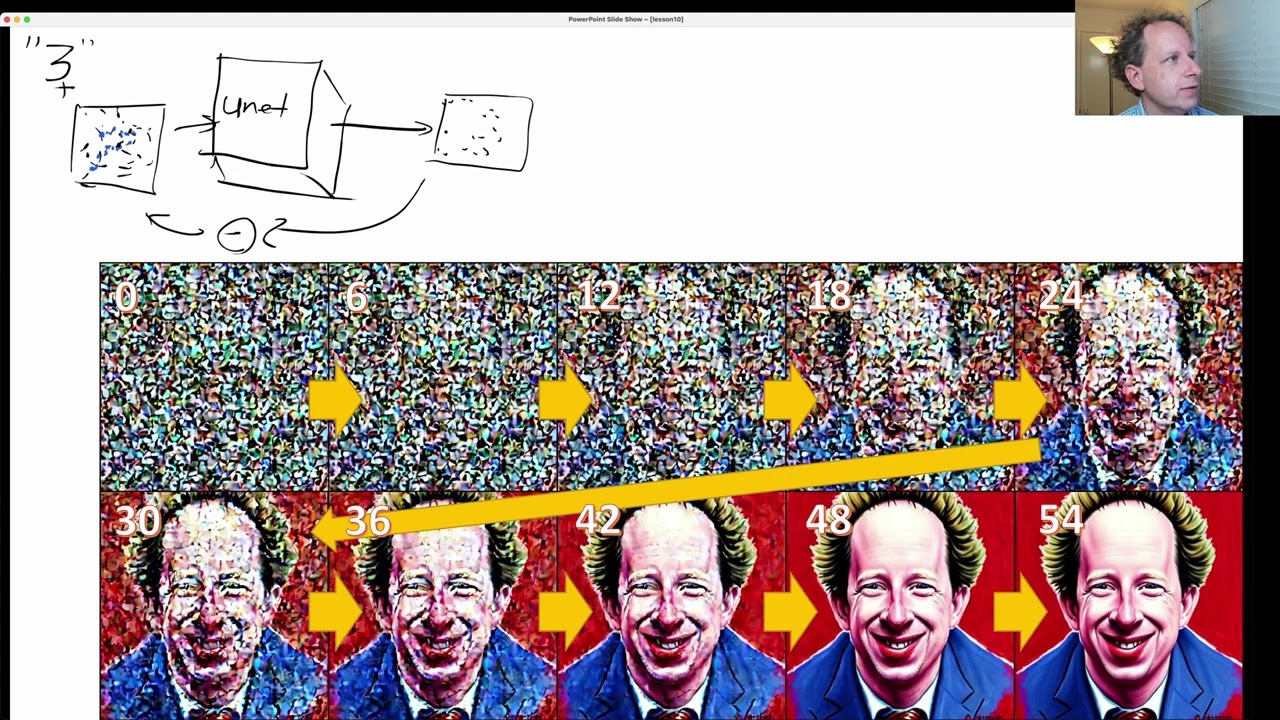
Initially, it's going to do quite a bad job of that. So we subtract just a little bit of that noise from the image to make it a little bit less noisy, and we do it again, and we do it a bunch of times. So here's what that looks like, creating a-- I think somebody here did a smiling picture of Jeremy Howard or something, if I remember correctly.

And if we print out the noise at kind of step zero, and it's step six, and it's step 12, you can see the first signs of a face starting to appear. Definitely a face appearing here, 18, 24. By step 30, it's looking much more like a face. By 42, it's getting there.

It's just got a few little blemishes to fix up. And here we are. I think I've slightly messed up my indexes here because it should finish at 60, not 54, but such is life. So rather rosy red lips, too, I would have to say. So remember, in the early days, this took 1,000 steps, and now there are some shortcuts to make it take 60 steps.

And this is what the process looks like. And the reason this doesn't look like normal noise is because now we are actually doing the VAE Latents thing. And so noisy Latents don't look like a Gaussian noise. They look like, well, they look like this. This is what happens when you decode those noisy Latents.

Now, you might remember last week I complained that things are moving too quickly. And there was a couple of papers that had come out the day before and made everything entirely out of date. So John and I and the team have actually had time to read those papers. And I thought now would be a good time to start going through some papers for the first time.

So what we're actually going to do is show how these papers have taken the required number of steps to go through this process down from 60 steps to 4 steps, which is pretty amazing. So let's talk about that. And the paper is specifically is this one progressive distillation for fast sampling of diffusion models.

So it's only been a week, so I haven't had much of a chance to try to explain this before. So apologies in advance if this is awkward, but hopefully it's going to make some sense. What we're going to start with is so we're going to start with this process, which is gradually denoising images and actually I wonder if we can copy it.

Okay, so how are we going to get this down from 60 steps to 4 steps? The basic idea is that we're going to do a process. We're going to do a process called distillation, which I have no idea how to spell, but hopefully that's close enough that you get the idea.

Distillation is a process which is pretty common in deep learning. And the basic idea of distillation is that you take something called a teacher network, which is some neural network that already knows how to do something, but it might be slow and big. And the teacher network is then used by a student network, which tries to learn how to do the same thing, but faster or with less memory.

And in this case, we want ours to be faster. We want to do less steps. And the way we can do this conceptually, it's actually, in my opinion, reasonably straightforward. We have. Like when I look at this and I think like, wow, you know, neural nets are really amazing.

So given your own, it's really amazing. Why is it taking like 18 steps to go from there to there? Like that seems like something that you should be able to do in one step. The fact that it's taking 18 steps and originally, of course, that was hundreds and hundreds of steps is because it's kind of that's just a kind of a side effect of the math of how this thing was originally developed, you know, this idea of this diffusion process.

But the idea in this paper is something that actually we've, I think I might have even mentioned in the last lesson, it's something we were thinking of doing ourselves before this paper beat us to it, which is to say, well, what if we train a new model where the model takes as input this image, right, and puts it through some other unit, unit B.

Okay. And then that spits out some result. And what we do is we take that result and we compare it to this image, the thing we actually want. Because the nice thing is now, which we've never really had before is we have for each intermediate output, like the desired goal where we're trying to get to.

And so we could compare those two just using, you know, whatever means squared error. Keep on forgetting to change my pen means squared error. And so then if we keep doing this for lots and lots of images and lots of lots of pairs and exactly this way, this unit is going to hopefully learn to take these incomplete images and turn them into complete images.

And that is exactly what this paper does. It just says, okay, now that we've got all these examples of showing what step 36 should turn into at step 54, let's just feed those examples into a model. And that works. And you'd kind of expect it to work because you can see that like a human would be able to look at this.

And if they were a competent artist, they could turn that into a, you know, a well finished product. So you would expect that a computer could as well. There are some little tweaks around how it makes this work, which I will briefly describe because we need to be able to go from kind of step one through to step 10 through to step 20 and so forth.

And so the way that it does this, it's actually quite clever. What they do is they initially, so they take their teacher model. So remember the teacher model is one that has already been trained. Okay. So the teacher model already is a complete stable diffusion model. That's finished. We take that as a given and we put in our image.

Well, actually it's noise. We put in our noise, right? And we put it through two time steps. Okay. And then we train our unit B or whatever you want to call it to try to go directly from the noise to time step number two. And it's pretty easy for it to do.

And so then what they do is they take this. Okay. And so this thing here, remember is called the student model. They then say, okay, let's now take that student model and treat that as the new teacher. So they now take their noise and they run it through the student model twice, once and twice, and they get out something at the end.

And so then they try to create a new student, which is a copy of the previous student, and it learns to go directly from the noise to two goes of the student model. And you won't be surprised to hear they now take that new student model and use that to go two goes.

And then they learn, they use that. Then they copy that to become the next student model. And so they're doing it again and again and again. And each time they're basically doubling the amount of work. So it goes one to two, effectively it's then going two to four and then four to eight.

And that's basically what they're what they're doing. And they're doing it for multiple different time steps. So the single student model is learning to both do these initial steps, trying to jump multiple steps at a time. And it's also learning to do these later steps, multiple steps at a time.

And that's it, believe it or not. So this is this neat paper that came out last week. And that's how it works. Now I mentioned that there was actually two papers. The second one is called On Distillation of Guided Diffusion Models. And the trick now is this second paper, these came out at basically the same time, if I remember correctly, even though they build on each other from the same teams, is that they say, okay, this is all very well, but we don't just want to create random pictures.

We want to be able to do guidance, right? And you might remember, I hope you remember from last week that we used something called Classifier Free Guided Diffusion Models, which, because I'm lazy, we will just use an acronym, Classifier Free Guided Diffusion Models. And this one, you may recall, we take, let's say we want a cute puppy.

We put in the prompt cute puppy into our clip text encoder, and that spits out an embedding. And we put that, let's ignore the VAE Latents business. We put that into our unit, but we also put the empty prompt into our clip text encoder. We concatenate these things too together so that then out the other side, we get back two things.

We get back the image of the cute puppy, and we get back the image of some arbitrary thing. Could be anything. And then we effectively do something very much like taking the weighted average of these two things together, combine them. And then we use that for the next stage of our diffusion process.

Now, what this paper does is it says, this is all pretty awkward. We end up having to train two images instead of one. And for different types of levels of guided diffusion, we have to do it multiple different times. It's all pretty annoying. How do we skip it? And based on the description of how we did it before, you may be able to guess.

What we do is we do exactly the same student-teacher distillation we did before, but this time we pass in, in addition, the guidance. And so again, we've got the entire stable diffusion model, the teacher model available for us. And we are doing actual CFGD, Classifier Free Guided Diffusion, to create our guided diffusion cute puppy pictures.

And we're doing it for a range of different guidance scales. So you might be doing two in 7.5 and 12 and whatever, right? And those now are becoming inputs to our student model. So the student model now has additional inputs. It's getting the noise as always. It's getting the caption or the prompt, I guess I should say, as always, but it's now also getting the guidance scale.

And so it's learning to find out how all of these things are handled by the teacher model. Like what does it do after a few steps each time? So it's exactly the same thing as before, but now it's learning to use the Classifier Free Guided Diffusion as well. Okay.

So that's got quite a lot going on there. And if it's a bit confusing, that's okay. It is a bit confusing. And what I would recommend is you check out the extra information from Jono who has a whole video on this. And one of the cool things actually about this video is it's actually a paper walkthrough.

And so part of this course is hopefully we're going to start reading papers together. Reading papers is extremely intimidating and overwhelming for all of us, all of the time, at least for me, it never gets any better. There's a lot of math. And by watching somebody like Jono, who's an expert at this stuff, read through a paper, you'll kind of get a sense of how he is skipping over lots of the math, right?

To focus on, in this case, the really important thing, which is the actual algorithm. And when you actually look at the algorithm, you start to realize it's basically all stuff, nearly all stuff, maybe all stuff that you did in primary school or secondary school. So we've got division, okay, sampling from a normal distribution, so high school, subtraction, division, division, multiplication, right?

Oh, okay, we've got a log there. But basically, you know, there's not too much going on. And then when you look at the code, you'll find that once you turn this into code, of course, it becomes even more understandable if you're somebody who's more familiar with code, like me.

So yeah, definitely check out Jono's video on this. So another paper came out about three hours ago. And I just had to show you it to you because I think it's amazing. And so this is definitely the first video about this paper because yeah, only came out a few hours ago.

But check this out. This is a paper called iMagic. And with this algorithm, you can pass in an input image. This is just a, you know, a photo you've taken or downloaded off the internet. And then you pass in some text saying a bird spreading wings. And what it's going to try to do is it's going to try to take this exact bird in this exact pose and leave everything as similar as possible, but adjust it just enough so that the prompt is now matched.

So here we take this, this little guy here, and we say, oh, this is actually what we want this to be a person giving the thumbs up. And this is what it produces. And you can see everything else is very, very similar to the previous picture. So this dog is not sitting.

But if we put in the prompt, a sitting dog, it turns it into a sitting dog, leaving everything else as similar as possible. So here's an example of a waterfall. And then you say it's a children's drawing of a waterfall and now it's become a children's drawing. So lots of people in the YouTube chat going, oh my God, this is amazing, which it absolutely is.

And that's why we're going to show you how it works. And one of the really amazing things is you're going to realize that you understand how it works already. Just to show you some more examples, here's the dog image. Here's the sitting dog, the jumping dog, dog playing with the toy, jumping dog holding a frisbee.

Okay. And here's this guy again, giving the thumbs up, crossed arms in a greeting pose to namaste hands, holding a cup. So that's pretty amazing. So I had to show you how this works. And I'm not going to go into too much detail, but I think we can get the idea actually pretty well.

So what we do is again, we start with a fully pre-trained, ready to go generative model like a stable diffusion model. And this is what this is talking about here, pre-trained diffusion model. In the paper, they actually use a model called Imogen, but none of the details as far as I can see in any way depend on what the model is.

It should work just fine for stable diffusion. And we take a photo of a bird spreading wings. Okay. So that's our, that's our target. And we create an embedding from that using, for example, our clip encoder as usual. And we then pass it through our pre-trained diffusion model. And we then see what it creates.

And it doesn't create something that's actually like our bird. So then what they do is they fine-tune this embedding. So this is kind of like textual inversion. They fine-tune the embedding to try to make the diffusion model output something that's as similar as possible to the, to the input image.

And so you can see here, they're saying, oh, we're moving our embedding a little bit. They don't do this for very long. They just want to move it a little bit in the right direction. And then now they lock that in place and they say, okay, now let's fine-tune the entire diffusion model end to end, including the VAE or actually with Imogen, they have a super resolution model, but same idea.

So we fine-tune the entire model end to end. And now the embedding, this optimized embedding we created, we, we, we store in place. We don't change that at all. That's now frozen. And we try to make it so that the diffusion model now spits out our bird as close as possible.

So you fine-tune that for a few epochs. And so you've now got something that takes this, embedding that we fine-tuned, goes through a fine-tuned model and spits out our bird. And then finally, the original target embedding we actually wanted is a photo of a bird spreading its wings. We ended up with this slightly different embedding and we take the weighted average of the two.

That's called the interpolate step, the weighted average of the two. And we pass that through this fine-tune diffusion model and we're done. And so that's pretty amazing. This, this would not take, I don't think a particularly long time or require any particular special hardware. It's the kind of thing I expect people will be doing, yeah, in the coming days and weeks.

But it's very interesting because, yeah, I mean, the ability to take any photo of a person or whatever and change it, like literally change what the person's doing is, you know, societally very important and really means that anybody I guess now can generate believable photos that never actually existed.

I see John O in the chat saying it took about eight minutes to do it for Imogen on TPUs. Although Imogen is quite a slow big model, although the TPUs they used were very, the latest TPUs. So might be, you know, maybe it's an hour or something for stable diffusion on GPUs.

All right. So that is a lot of fun. All right. So with that, let's go back to our notebook where we left it last time. We had kind of looked at some applications that we can play with in this diffusion NBS repo, in the stable diffusion notebook. And what we've got now, and to remind you, when I say we, it's mainly actually Pedro, Patrick and Suraj, just a little bit of help from me.

So hugging face folks. What we/they have done is they now dig into the pipeline to pull it all apart step by step. So you can see exactly what happens. The first thing I was just going to mention is this is how you can create those gradual denoising pictures. And this is thanks to something called the callback.

So you can say here, when you go through the pipeline, every 12 steps, call this function. And as you can see, it's going to call it with I and T and the latents. And so then we can just make an image and stick it on the end of an array.

And that's all that's happening here. So this is how you can start to interact with a pipeline without rewriting it yourself from scratch. But now what we're going to do is we're actually going to write it, we're going to build it from scratch. So you don't actually have to use a callback because you'll be able to change it yourself.

So let's take a look. So looking inside the pipeline, what exactly is going on? So what's going to be going on in the pipeline is seeing all of the steps that we saw in last week's OneNote notes that I drew. And it's going to be all the code. And we're not going to show the code of how each step is implemented.

So for example, the clip text model we talked about, the thing that takes as input a prompt and creates an embedding, we just take that as a given. So we download it, open AI is trained one called clip, the IT large patch 14. So we just say from tree change.

So hugging face will transformers will download and create that model for us. Ditto for the tokenizer. And so ditto for the auto encoder, and ditto for the unit. So there they all are, we can just grab them. So we just take that all as a given. These are the three models that we've talked about, the text encoder, the clip encoder, the VAE, and the unit.

So there they are. So given that we now have those, the next thing we need is that thing that converts time steps into the amount of noise. Remember that graph we drew. And so we can basically, again, use something that hugging face, well, actually, in this case, Catherine Carlson has already provided, which is a scheduler, it's basically something that shows us that connection.

So we've got that. So we use that scheduler. And we say how much noise when we're using. And so we have to make sure that that matches. And so we just use these numbers that were given. Okay, so now to create our photograph of astronaut riding a horse again, in 70 steps with a 7.5 guide and scale, batch size of one, step number one is to take our prompt and tokenize it.

Okay, so we looked at that in part one of the course. So check that out if you can't remember what tokenizing does, but it's just splitting it in basically splitting it into words, or subword units if they're long and unusual words. So here are so this will be the start the start of sentence token, and this will be a photograph of an astronaut, etc.

And then you can see the same token is repeated again again at the end. That's just the padding to say we're all done. And the reason for that is that GPUs and TPUs really like to do lots of things at once. So we kind of have everything be the same length by padding them.

That may sound like a lot of wasted work, which it kind of is. But a GPU would rather do lots of things at the same time on exactly the same sized input. So this is why we have all this padding. So you can see here if we decode that number, it's the end of text marker, just just padding really in this case.

As well as getting the input IDs, so these are just lookups into a vocabulary. There's also a mask, which is just telling it which ones are actual words as opposed to padding, which is not very interesting. So we can now take those input IDs, we can put them on the GPU, and we can run them through the clip encoder.

And so for a batch size of one, so you've got one image that gives us back a 77 by 768, because we've got 77 here. And each one of those creates a 768 long vector. So we've got a 77 by 768 tensor. So these are the embeddings for a photograph of an astronaut riding a horse that come from clip.

So remember, everything's pre-trained. So that's all done for us. We're just doing inference. And so remember, for the classifier free guidance, we also need the embeddings for the empty string. So we do exactly the same thing. So now we just concatenate those two together, because this is just a trick to get the GPU to do both at the same time, because we like the GPU to do as many things at once as possible.

And so now we create our noise. And because we're doing it with a VAE, we can call it Latents, but it's just noise, really. I wonder if you'd still call it that without the VAE. Maybe you would have to think about that. So that's just random numbers normally generated, normally distributed random numbers of size one, that's our batch size.

And the reason that we've got this divided by eight here is because that's what the VAE does. It allows us to create things that are eight times smaller by height and width. And then it's going to expand it up again for us later. That's why this is so much faster.

You'll see a lot of this after we put it on the GPU, you'll see a lot of this dot half. This is converting things into what's called half precision or FB 16. Details don't matter too much. It's just making it half as big in memory by using less precision.

Modern GPUs are much, much, much, much faster if we do that. So you'll see that a lot. If you use something like fast AI, you don't have to worry about it, but all this stuff is done for you. And we'll see that later as we rebuild this with much, much less code later in the course.

So we'll be building our own kind of framework from scratch, which you'll then be able to maintain and work with yourself. Okay, so we have to say we want to do 70 steps. Something that's very important, we won't worry too much about the details right now, but what you see here is that we take our random noise and we scale it.

And that's because depending on what stage you're up to, you need to make sure that you have the right amount of variance, basically. Otherwise you're going to get activations and gradients that go out of control. This is something we're going to be talking about a huge amount during this course, and we'll show you lots of tricks to handle that kind of thing automatically.

Unfortunately at the moment in the stable diffusion world, this is all done in rather, in my opinion, kind of ways that are too tied to the details of the model. I think we will be able to improve it as the course goes on, but for now we'll stick with how everybody else is doing it.

This is how they do it. So we're going to be jumping through. So normally it would take a thousand time steps, but because we're using a fancy scheduler, we get to skip from 999 to 984, 984 to 970, and so forth. So we're going down about 14 time steps.

And remember, this is a very, very, very unfortunate word. They're not time steps at all. In fact, they're not even integers. It's just a measure of how much noise are we adding at each time, and you find out how much noise by looking it up on this graph. Okay.

That's all time step means. It's not a step of time, and it's a real shame that that word is used because it's incredibly confusing. This is much more helpful. This is the actual amount of noise at each one of those iterations. And so here you can see the amount of noise for each of those time steps, and we're going to be going backwards.

As you can see, we start at 999, so we'll start with lots of noise, and then we'll be using less and less and less and less noise. So we go through the 70 time steps in a for loop, concatenating our two noise bits together, because we've got the classifier free and the prompt versions, do our scaling, calculate our predictions from the unit, and notice here we're passing in the time step, as well as our prompt.

That's going to return two things, the unconditional prediction, so that's the one for the empty string. Remember, we passed in one of the two things we passed in was the empty string. So we concatenated them together, and so after they come out of the unit, we can pull them apart again.

So dot chunk just means pull them apart into two separate variables, and then we can do the guide and scale that we talked about last week. And so now we can do that update where we take a little bit of the noise and remove it to give us our new latents.

So that's the loop. And so at the end of all that, we decode it in the VAE. The paper that created this VAE tells us that we have to divide it by this number to scale it correctly. And once we've done that, that gives us a number which is between negative one and one.

Python imaging library expects something between zero and one, so that's what we do here to make it between zero and one and enforce that to be true. Put that back on the CPU, make sure it's that the order of the dimensions is the same as what Python imaging library expects, and then finally convert it up to between zero and 255 as an int, which is actually what PIO really wants.

And there's our picture. So there's all the steps. So what I then did, this is kind of like, so the way I normally build code, I use notebooks for everything, is I kind of do things step by step by step, and then I tend to kind of copy them, and I use shift M.

I don't know if you've seen that, but what shift M does, it takes two cells and combines them like that. And so I basically combined some of the cells together, and I removed a bunch of the the pros, so you can see the entire thing on one screen. And what I was trying to do here is I'd like to get to the point where I've got something which I can very quickly do experiments with.

So maybe I want to try some different approach to guidance tree classification, maybe I want to add some callbacks, so on and so forth. So I kind of like to have everything, you know, I like to have all of my important code be able to fit into my screen at once.

And so you can see now I do, I've got the whole thing on my screen, so I can keep it all in my head. One thing I was playing around with was I was trying to understand the actual guidance tree equation in terms of like how does it work.

Computer scientists tend to write things and software engineers with kind of long words as variable names. Mathematicians tend to use short just letters normally. For me, when I want to play around with stuff like that, I turn stuff back into letters. And that's because I actually kind of pulled out one note and I started jutting down this equation and playing around with it to understand how it behaves.

So this is just like, it's not better or worse, it's just depending on what you're doing. So actually here I said, okay, g is guidance scale. And then rather than having the unconditional and text embeddings, I just call them u and t. And now I've got this all down into an equation which I can write down in a notebook and play with and understand exactly how it works.

So that's something I find really helpful for working with this kind of code is to, yeah, turn it into a form that I can manipulate algebraically more easily. I also try to make it look as much like the paper that I'm implementing as possible. Anyways, that's that code. So then I copied all this again and I basically, oh, I actually did it for two prompts this time.

I thought this was fun. While you're painting an astronaut riding a horse in the style of Grant Wood, just to remind you, Grant Wood looks like this. Not obviously astronaut material, which I thought would make it actually kind of particularly interesting. Although he does have horses. I can't see one here.

Some of his pictures have horses. So because I did two prompts, I got back two pictures I could do. So here's the Grant Wood one. I don't know what's going on in his back here, but I think it's quite nice. So yeah, I then copied that whole thing again and merged them all together and then just put it into a function.

So I took the little bit which creates an image and put that into a function. I took the bit which does the tokenizing and text encoding and put that into a function. And so now all of the code necessary to do the whole thing from top to bottom fits in these two cells, which makes it for me much easier to see exactly what's going on.

So you can see I've got the text embeddings. I've got the unconditional embeddings. I've got the embeddings which can catenate the two together, optional random seed, my latents, and then the loop itself. And you'll also see something I do which is a bit different to a lot of software engineering is I often create things which are kind of like longer lines because I try to have each line be kind of like mathematically one thing that I want to be able to think about as a whole.

So yeah, these are some differences between kind of the way I find numerical programming works well compared to the way I would write a more traditional software engineering approach. And again, this is partly a personal preference, but it's something I find works well for me. So we're now at a point where we've got, yeah, two fun, three functions that easily fit on the screen and do everything.

So I can now just say make samples and display each image. And so this is something for you to experiment with. And what I specifically suggest as homework is to try picking one of the extra tricks we learned about like image to image or negative prompts. Negative prompts would be a nice easy one like see if you can implement negative prompt in your version of this.

Or yeah, try doing image to image. That wouldn't be too hard either. Another one you can add is try adding callbacks. And the nice thing is then, you know, you've got code which you fully understand because you know what all the lines do. And you then don't need to wait for the diffusers folks to update it.

The library to do is, for example, the callbacks are only added like a week ago. So until then you couldn't do callbacks. Well, now you don't have to wait for the diffusers team to add something. The code's all here for you to play with. So that's my recommendation as a bit of homework for this week.

Okay, so that brings us to the end of our rapid overview of stable diffusion and some very recent papers that very significantly developed stable diffusion. I hope that's given you a good sense of the kind of very high level slightly hand wavy version of all this and you can actually get started playing with some fun code.

What we're going to be doing next is going right back to the start, learning how to multiply two matrices together effectively and then gradually building from there until we've got to the point that we've rebuilt all this from scratch and we understand why things work the way they do, understand how to debug problems, improve performance and implement new research papers as well.

So that's going to be very exciting. And so we're going to have a break and I will see you back here in 10 minutes. Okay, welcome back everybody. I'm really excited about the next part of this. It's going to require some serious tenacity and a certain amount of patience.

But I think you're going to learn a lot. A lot of folks I've spoken to have said that previous iterations of this part of the course is like the best course they've ever done. And this one's going to be dramatically better than any previous version we've done of this.

So hopefully you'll find that the hard work and patience pays off. We're working now through the course 22 p2 repo. So 2022 course part two. And notebooks are ordered. So we'll start with notebook number one. And okay, so the goal is to get to stable diffusion from the foundations, which means we have to define what are the foundations.

So I've decided to define them as follows. We're allowed to use Python. We're allowed to use the Python standard library. So that's all the stuff that comes with Python by default. We're allowed to use matplotlib because I couldn't be bothered creating my own plotting library. And we're allowed to use Jupyter notebooks and NBDev, which is something that creates modules from notebooks.

So basically what we're going to try to do is to rebuild everything starting from this foundation. Now, to be clear, what we are allowed to use are the libraries once we have reimplemented them correctly. And so if we reimplement something from NumPy or PyTorch or whatever, we're then allowed to use the NumPy or PyTorch or whatever version.

Sometimes we'll be creating things that haven't been created before. And that's then going to be becoming our own library. And we're going to be calling that library mini AI. So we're going to be building our own little framework as we go. So, for example, here are some imports. And these imports all come from the Python standard library, except for these two.

Now, to be clear, one challenge we have is that the models we use in stable diffusion were trained on millions of dollars worth of equipment for months, which we don't have the time or money. So another trick we're going to do is we're going to create smaller identical but smaller versions of them.

And so once we've got them working, we'll then be allowed to use the big pre-trained versions. So that's the basic idea. So we're going to have to end up with our own VAE, our own unit, our own clip encoder, and so forth. To some degree, I am assuming that you've completed part one of the course.

To some degree, I will cover everything at least briefly. But if I cover something about deep learning too fast for you to know what's going on and you get lost, go back and watch part one, or go and Google for that term. For stuff that we haven't covered in part one, I will go over it very thoroughly and carefully.

All right. So I'm going to assume that you know the basic idea, which is that we're going to need to be doing some matrix multiplication. So we're going to try to take a deep dive into matrix multiplication today. And we're going to need some input data. And I quite like working with MNIST data.

MNIST is handwritten digits. It's a classic data set. They're 28 by 28 pixel grayscale images. And so we can download them from this URL. So we use the path libs path object a lot. It's part of Python. And it basically takes a string and turns it into something that you can treat as a path.

For example, you can use slash to mean this file inside this subdirectory. So this is how we create a path object. Path objects have, for example, a make directory method. So I like to get everything set up. But I want to be able to rerun this cell lots of times and not give me errors if I run it more than once.

If I run it a second time, it still works. And in that case, that's because I put this exist OK equals true. How did I know that I can say-- because otherwise, it would try to make the directory. It would already exist in a given error. How do I know what parameters I can pass to make dir?

I just press shift tab. And so when I hit shift tab, it tells me what options there are. If I press it a few times, it'll actually pop it down to the bottom of the screen to remind me. I can press escape to get rid of it. Or you can just-- or else you can just hit tab inside.

And it'll list all the things you could type here, as you can see. All right. So we need to grab this URL. And so Python comes with something for doing that, which is the URL lib library that's part of Python that has something called URL retrieve. And something which I'm always a bit surprised is not widely used as people reading the Python documentation.

So you should do that a lot. So if I click on that, here is the documentation for URL retrieve. And so I can find exactly what it can take. And I can learn about exactly what it does. And so I read the documentation from the Python docs for every single method I use.

And I look at every single option that it takes. And then I practice with it. And to practice with it, I practice inside Jupyter. So if I want this import on its own, I can hit Control-Shift- and it's going to spit it into two cells. And then I'll hit Alt-Enter or Option-Enter so I can create something underneath.

And I can type URL retrieve, Shift-Tab. And so there it all is. If I'm like way down somewhere in the notebook and I have no idea where URL retrieve comes from, I can just hit Shift-Enter. And it actually tells me exactly where it comes from. And if I want to know more about it, I can just hit Question Mark, Shift-Enter, and it's going to give me the documentation.

And most cool of all, second question mark, and it gives me the full source code. And you can see it's not a lot. You know, reading the source code of Python standard library stuff is often quite revealing. And you can see exactly how they do it. And that's a great way to learn more about more about this.

So in this case, I'm just going to use a very simple functionality, which is I'm going to say the URL to retrieve and the file name to save it as. And again, I made it so I can run this multiple times. So it's only going to do the URL retrieve if the path doesn't exist.

If I've already downloaded it, I don't want to download it again. So I run that cell. And notice that I can put exclamation mark, followed by a line of bash. And it actually runs this using bash. If you're using Windows, this won't work. And I would very, very strongly suggest if you're using Windows, use WSL.

And if you use WSL, all of these notebooks will work perfectly. So yeah, do that. Or write it on paper space or Lambda Labs or something like that, Colab, et cetera. Okay, so this is a gzip file. So thankfully, Python comes with a gzip module. Python comes with quite a lot, actually.

And so we can open a gzip file using gzip.open. And we can pass in the path. And we'll say we're going to read it as binary as opposed to text. Okay, so this is called a context manager. It's a with clause. And what it's going to do is it's going to open up this gzip file.

The gzip object will be called f. And then it runs everything inside the block. And when it's done, it will close the file. So with blocks can do all kinds of different things. But in general, with blocks that involve files are going to close the file automatically for you.

So we can now do that. And so you can see it's opened up the gzip file. And the gzip file contains what's called pickle objects. Pickled objects is basically Python objects that have been saved to disk. It's the main way that people in pure Python save stuff. And it's part of the standard library.

So this is how we load in from that file. Now, the file contains a tuple of tuples. So when you put a tuple on the left hand side of an equal sign, it's quite neat. It allows us to put the first tuple into two variables called x_train and y_train and the second into x_valid and y_valid.

This trick here where you put stuff like this on the left is called destructuring. And it's a super handy way to make your code kind of clear and concise. And lots of languages support that, including Python. Okay. So we've now got some data. And so we can have a look at it.

Now, it's a bit tricky because we're not allowed to use NumPy according to our rules. But unfortunately, this actually comes as NumPy. So I've turned it into a list. All right. So I've taken the first image and I've turned it into a list. And so we can look at a few examples of some values in that list.

And here they are. So it looks like they're numbers between zero and one. And this is what I do when I learn about a new dataset. So when I started writing this notebook, what you see here, other than the pros here, is what I actually did when I was working with this data.

I wanted to know what it was. So I just grab a little bit of it and look at it. So I kind of got a sense now of what it is. Now, interestingly, it's 784. This image is 784 long list. Oh, dear. People freaking out in the comments. No NumPy.

Yeah. No NumPy. Do you see NumPy? No NumPy. Why 784? What is that? Well, that's because these are 28 by 28 images. So it's just a flat list here of 784 long. So how do I turn this 784 long thing into 28 by 28? So I want a list of 28 lists of 28, basically, because we don't have matrices.

So how do we do that? And so we're going to be learning a lot of cool stuff in Python here. Sorry, I can't stop laughing at all the stuff in our chat. Oh, dear. People are quite reasonably freaking out. That's okay. We'll get there. I promise. I hope. Otherwise, I'll embarrass myself.

All right. So how do I convert a 784 long list into 28 lists, 28 long list of 28 long lists? I'm going to use something called chunks. And first of all, I'll show you what this thing does. And then I'll show you how it works. So vowels is currently a list of 10 things.

Now, if I take vowels and I pass it to chunks with five, it creates two lists of five. Here's list number one of five elements. And here's list number two of five elements. Hopefully, you can see what it's doing. It's chunkifying this list. And this is the length of each chunk.

Now, how did it do that? The way I did it is using a very, very useful thing in Python that far too many people don't know about, which is called yield. And what yield does is you can see here, if we're on loop, it's going to go through from zero up to the length of my list.

And it's going to jump by five at a time. It's going to go, in this case, zero comma five. And then it's going to think of this as being like return for now, it's going to return the list from zero up to five. So it returns the first bit of the list.

But yield doesn't just return. It kind of like returns a bit and then it continues. And it returns a bit more. And so specifically, what yield does is it creates an iterator. An iterator is an iterator is basically something you can actually use it that you can call next on a bunch of times.

So let's try it. So we can say iterator equals. Okay. Oh, got to run it. So what is iterator? Well, iterator is something that I can basically, I can call next on. And next basically says yield the next thing. So this should yield vals zero colon five. There it is.

It did, right? There's vals zero colon five. Now, if I run that again, it's going to give me a different answer because it's now up to the second part of this loop. Now it returns the last five. Okay. So this is what an iterator does. Now, if you pass an iterator to Python's list, it runs through the entire iterator until it's finished and creates a list of the results.

And what does finished looks like? This is what finished looks like. If you call next and get stop iteration, that means you've run out. And that makes sense, because my loop, there's nothing left in it. So all of that is to say, we now have a way of taking a list and chunkifying it.

So what if I now take my full image, image number one, chunkify it into chunks of 28 long and turn that into a list and plot it. We have successfully created an image. So that's good. Now, we are done. But there are other ways to create this iterator. And because iterators and generators, which are closely related, so important, I wanted to show you more about how to do them in Python.

It's one of these things that if you understand this, you'll often find that you can throw away huge pieces of enterprise software and basically replace it with an iterator. It lets you stream things one bit at a time. It doesn't store it all in memory. It's this really powerful thing that once I show it to people, they suddenly go like, oh, wow, we've been using all this third party software and we could have just created a Python iterator.

Python comes with a whole standard library module called edit tools just to make it easier to work with iterators. I'll show you one example of something from edit tools, which is iseless. So let's grab our values again, these 10 values. Okay. So let's take these 10 values and we can take any list and turn it into an iterator by passing it to itter, which I should call it.

So I don't override this Python. That's not a keyword, but this thing I don't want to override. So this is now basically something that I can call. Actually, let's do this. I'll show you that I can call next on it. So if I now go next it, you can see it's giving me each item one at a time.

Okay. So that's what converting it into an iterator does. I slice, converts it into a different kind of iterator. Let's call this maybe I slice iterator. And so you can see here, what it did was it jumped. Stop here. So that's what had been better. So I should query, create the iterator and then call next a few times.

Sorry. This is what I went to do. It's now only returning the first five before it calls stop iteration before it raises stop iteration. So what I slice does is it grabs the first N things from an iterable, something that you can iterate. Why is that interesting? Because I can pass it to list for example.

Right. And now if I pass it to list again, this iterator has now grabbed the first five things. So it's now up to thing number six. So if I call it again, it's the next five things. And if I call it again, then there's nothing left. And maybe you can see we've actually now got this defined, but we can do it with I slice.

And here's how we can do it. It's actually pretty tricky. It in Python, you can pass it something like a list to create an iterator, or you can pass it. Now this is a really important word. A callable. What's a callable? A callable is generally speaking, it's a function.

It's something that you can put parentheses after. Could even be a class. Anything you can put parentheses after, you can just think of it for now as a function. So we're going to pass it a function. And in the second form, it's going to be called until the function returns this value here, which in this case is empty list.

And we just saw that I slice will return empty list when it's done. So this here is going to keep calling this function again and again and again. And we've seen exactly what happens because we've called it ourselves before. There it is. Until it gets an empty list. So if we do it with 28, then we're going to get our image again.

So we've now got two different ways of creating exactly the same thing. And if you've never used iterators before, now's a good time to pause the video and play with them, right? So for example, you could take this here, right? And if you've not seen lambdas before, they're exactly the same as functions, but you can define them in line.

So let's replace that with a function. Okay, so now I've turned it into a function and then you can experiment with it. So let's create our iterator and call f on it. Well, not on it, call f. And you can see there's the first 28. And each time I do it, I'm getting another 28.

Now the first two rows are all empty, but finally, look, now I've got some values. Call it again. See how each time I'm getting something else. Just calling it again and again. And that is the values in our iterator. So that gives you a sense of like how you can use Jupyter to experiment.

So what you should do is as soon as you hit something in my code that doesn't look familiar to you, I recommend pausing the video and experimenting with that in Jupyter. And for example, itter, most people probably have not used itter at all, and certainly very few people have used this to argument form.

So hit shift tab a few times, and now you've got at the bottom, there's a description of what it is. Or find out more. Python itter. Here we are, go to the docs. Well, that's not the right bit of the docs. See API? Wow, crazy. That's terrible. Let's try searching here.

There we go. That's more like it. So now you've got links. So if it's like, okay, it returns an iterator object, what's that? Well, click on it. Find out. Now this is really important to know. And here's that stop exception that we saw. So stop iteration exception. We saw next already.

We can find out what iterable is. And here's an example. And as you can see, it's using exactly the same approach that we did, but here it's being used to read from a file. This is really cool. Here's how to read from a file. 64 bytes at a time until you get nothing processing it, right?

So the docs of Python are quite fantastic. As long as you use them, if you don't use them, they're not very useful at all. And I see Seifer in the comments, our local Haskell programmer, appreciating this Haskellness in Python. That's good. It's not quite Haskell, I'm afraid, but it's the closest we're going to come.

All right. How are we going for time? Pretty good. Okay. So now that we've got image, which is a list of lists and each list is 25 long, we can index into it. So we can say image 20. Well, let's do it. Image 20. Okay. Is a list of 28 numbers.

And then we could index into that. Okay. So we can index into it. Now, normally, we don't like to do that for matrices. We would normally rather write it like this. Okay. So that means we're going to have to create our own class to make that work. So to create a class in Python, you write class, and then you write the name of it.

And then you write some really weird things. The weird things you write have two underscores, a special word, and then two underscores. These things with two underscores on each side are called dunder methods, and they're all the special magically named methods which have particular meanings to Python. And you're just going to learn them, but they're all documented in the Python object model.

Edit object model. Yay, finally. Okay. So it's called data model, not object model. And so this is basically where all the documentation is about absolutely everything, and I can click under edit, and it tells you basically this is the thing that constructs objects. So any time you want to create a class that you want to construct, it's going to store some stuff.

So in this case, it's going to store our image. You have to define dunder in it. Python's slightly weird in that every method, you have to put self here. For reasons we probably don't really need to get into right now. And then any parameters. So we're going to be creating an image passing in the thing to store, the Xs.

They're going to be passing in the Xs. And so here we're just going to store it inside the self. So once I've got this line of code, I've now got something that knows how to store stuff, the Xs inside itself. So now I want to be able to call square bracket 20 comma 15.

So how do we do that? Well, basically part of the data model is that there's a special thing called dunder get item. And when you call square brackets on your object, that's what Python uses. And it's going to pass across the 20 comma 15 here as indices. So we're now basically just going to return this.

So the self.Xs with the first index and the second index. So let's create that matrix class and run that. And you can now see M 20 comma 15 is the same. Oh, quick note on, you know, ways in which my code is different to everybody else's, which it is.

It's somewhat unusual to put definitions of methods on the same line as as the the signature like this. I do it quite a lot for one-liners. As I kind of mentioned before, I find it really helps me to be able to see all the code I'm working with on the screen at once.

A lot of the world's best programmers actually have had that approach as well. It seems to work quite well for some people that are extremely productive. It's not common in Python. Some people are quite against it. So if you're at work, and your colleagues don't write Python this way, you probably shouldn't either.

But if you can get away with it, I think it works quite well. Anyway, okay, so now that we've created something that lets us index into things like this, we're allowed to use PyTorch because we're allowed to use this one feature in PyTorch. Okay, so we can now do that.

And so now to create a tensor, which is basically a lot like our matrix, we can now pass a list into tensor to get back a tensor version of that list, or perhaps more interestingly, we could pass in a list of lists. Maybe let's give this a name. Whoopsie dozy.

That needs to be a list of lists, just like we had before for our image. In fact, let's do it for our image. Let's just pass in our image. There we go. And so now we should be able to say tens 20 comma 15. And there we go. Okay, so we've successfully reinvented that.

All right. So now we can convert all of our lists into tenses. There's a convenient way to do this, which is to use the map function in the Python standard library. So it takes a function and then some iterables. In this case, one iterable. And it's going to apply this function to each of these four things and return those four things.

And so then I can put four things on the left to receive those four things. So this is going to call tensor x_train and put it in x_train. Tensor y_train, put it in y_train, and so forth. So this is converting all of these lists to tenses and storing them back in the same name.

So you can see that x_train now is a tensor. So that means it has a shape property. It has 50,000 images in it, which are each 784 long. And you can find out what kind of stuff it contains by calling its .type. So it contains floats. So this is the tensor class.

We'll be using a lot of it. So of course, you should read its documentation. I don't love the PyTorch documentation. Some of it's good. Some of it's not good. It's a bit all over the place. So here's tensor. But it's well worth scrolling through to get a sense of like, this is actually not bad, right?

It tells you how you can construct it. This is how I constructed one before, passing it lists of lists. You can also pass it NumPy arrays. You can change types. So on and so forth. So, you know, it's well worth reading through. And like, you're not going to look at every single method it takes, but you're kind of, if you browse through it, you'll get a general sense, right?

That tensors do just about everything you couldn't think of for a numeric programming. At some point, you will want to know every single one of these, or at least be aware roughly what exists. So you know what to search for in the docs. Otherwise you will end up recreating stuff from scratch, which is much, much slower than simply reading the documentation to find out it's there.

All right. So instead of, instead of calling chunks or I slice, the thing that is roughly equivalent in a tensor is the reshape method. So reshape, so to reshape our 50,000 by 784 thing, we can simply, we want to turn it into 50,000 28 by 28 tensors. So I could write here, reshape to 50,000 by 28 by 28.

But I kind of don't need to, because I could just put minus one here and it can figure out that that must be 50, that must be 50,000 because it knows that I have 50,000 by 784 items. So it can figure out, so minus one means just fill this with all the rest.

Okay. Now, what does the word tensor mean? So there's some very interesting history here. And I'll try not to get too far into it because I'm a bit over enthusiastic about this stuff, I must admit. I'm very, very interested in the history of tensor programming and array programming. And it basically goes back to a language called APL.

APL is basically originally a mathematical notation that was developed in the mid to late 50s, 1950s. And at first it was used as a notation for defining how certain new IBM systems would work. So it was all written out in this notation. It's kind of like a replacement for mathematical notation that was designed to be more consistent and kind of more expressive.

In the early 60s, so the guy who wrote and made it was called his name Ken Iverson. In the early 60s, some implementations that actually allow this notation to be executed on a computer appeared. Both the notation and the executable implementations slightly confusingly are both called APL. APL's been in constant development ever since that time.

And today is one of the world's most powerful programming languages. And you can try it by going to try APL. And why am I mentioning it here? Because one of the things Ken Iverson did, well, he studied an area of physics called tensor analysis. And as he developed APL, he basically said like, oh, what if we took these ideas from tensor analysis and put them into a programming language?

So in APL, you can and have been able to for some time can basically you can define a variable. And rather than saying equals, which is a terrible way to define things really mathematically, because that has a very different meaning most of the time in math. Instead, we use arrow to define things.

We can say, okay, that's going to be a tensor like so. And then we can look at their contents of A and we can do things like, oh, what if we do A times three or A minus two and so forth. And as you can see, what it's doing is it's taking all the contents of this tensor and it's multiplying them all by three or subtracting two from all of them.

Or perhaps more fun, we could put into B a different tensor. And we can now do things like A divided by B. And you can see it's taking each of A and dividing by each of B. Now, this is very interesting because now we don't have to write loops anymore.

We can just express things directly. We can multiply things by scalars, even if they're, this is called a rank one tensor. That is to say it's basically in math, we'd call it a vector. We can take two vectors and can divide one by the other and so forth. It's a really powerful idea.

Funnily enough, APL didn't call them tensors, even though Ken Iverson said he got this idea from tensor analysis, APL calls them arrays. NumPy, which was heavily influenced by APL, also calls them arrays. For some reason, PyTorch, which is very heavily influenced by APL, sorry, by NumPy, doesn't call them arrays, it calls them tensors.

They're all the same thing. They are rectangular blocks of numbers. They can be one-dimensional, like a vector. They can be two-dimensional, like a matrix. They can be three-dimensional, which is like a bunch of stacked matrices, like a batch of matrices and so forth. If you are interested in APL, which I hope you are, we have a whole APL and array programming section on our forums, and also we've prepared a whole set of notes on every single glyph in APL, which also covers all kinds of interesting mathematical concepts, like complex direction and magnitude, and all kinds of fun stuff like that.

That's all totally optional, but a lot of people who do APL say that they feel like they've become a much better programmer in the process, and also you'll find here at the forums a set of 17 study sessions of an hour or two each, covering the entirety of the language, every single glyph.

That's all where this stuff comes from. This batch of 50,000 images, 50,000 28 by 28 images, is what we call a rank 3 tensor in PyTorch. In NumPy, we would call it an array with three dimensions. Those are the same thing. What is the rank? The rank is just the number of dimensions.

It's 50,000 images of 28 high by 28 wide, so there are three dimensions that is the rank of the tensor. If we then pick out a particular image, then we look at its shape, we could call this a matrix. It's a 28 by 28 tensor, or we could call it a rank 2 tensor.

A vector is a rank 1 tensor. In APL, a scalar is a rank 0 tensor, and that's the way it should be. A lot of languages and libraries don't, unfortunately, think of it that way. So what is a scalar? It's a bit dependent on the language. Okay, so we can index into the zeroth image, 20th row, 15th column to get back this same number.

Okay, so we can take x_train.shape, which is 50,000 by 784, and you can destructure it into n, which is the number of images, and c, which is the number of the full number of columns, for example. And we can also, well this is actually part of the standard library, so we're allowed to use min, so we can find out in y_train what's the smallest number, and what's the maximum number, so they go from 0 to 9.

So you see here, it's not just the number 0, it's a scalar tensor, 0. They act almost the same, most of the time. So here's some example of a bit of the y_train, so you can see these are basically, this is going to be the labels, right, these are our digits, and this is its shape, so there's just 50,000 of these labels.

Okay, and so since we're allowed to use this in the standard library, well it also exists in PyTorch, so that means we're also allowed to use the .min and .max properties. All right, so before we wrap up, we're going to do one more thing, and I don't know what the, we would call kind of anti-cheating, but according to our rules, we're allowed to use random numbers because there is a random number generator in the Python standard library, but we're going to do random numbers from scratch ourselves, and the reason we're going to do that is even though according to the rules we could be allowed to use the standard library one, it's actually extremely instructive to build our own random number generator from scratch, well at least I think so.

Let's see what you think. So there is no way normally in software to create a random number, unfortunately. Computers, you know, add, subtract, times, logic gates, stuff like that. So how does one create random numbers? Well you could go to the Australian National University Quantum Random Number Generator, and this looks at the quantum fluctuations of the vacuum and provides an API which will actually hook you in and return quantum random fluctuations of the vacuum.

So that's about, that's the most random thing I'm aware of, so that would be one way to get random numbers. And there's actually an API for that, so there's a bit of fun. You could do what Cloudflare does. Cloudflare has a huge wall full of lava lamps, and it uses the pixels of a camera looking at those lava lamps to generate random numbers.

Intel nowadays actually has something in its chips, which you can call rdrand, which will return random numbers on certain Intel chips from 2012. All of these things are kind of slow, they can kind of get you one random number from time to time. We want some way of getting lots and lots of random numbers, and so what we do is we use something called a pseudorandom number generator.

A pseudorandom number generator is a mathematical function that you can call lots of times, and each time you call it, it will give you a number that looks random. To show you what I mean by that, I'm going to run some code. I've created a function which we'll look at in a moment called rand, and if I call rand 50 times and plot it, there's no obvious relationship between one call and the next.

That's one thing that I would expect to see from my random numbers. I would expect that each time I call rand, the numbers would look quite different to each other. The second thing is, rand is meant to be returning uniformly distributed random numbers, and therefore if I call it lots and lots and lots of times and plot its histogram, I would expect to see exactly this, which is each from 0 to 0.1, there's a few, from 0.1 to 0.2, there's a few, from 0.2 to 0.3, there's a few.

It's a fairly evenly spread thing. These are the two key things I would expect to see, an even distribution of random numbers and that there's no correlation or no obvious correlation from one to the other. We're going to try and create a function that has these properties. We're not going to derive it from scratch.

I'm just going to tell you that we have a function here called the Wickman-Hill algorithm. This is actually what Python used to use back in before Python 2.3, and the key reason we need to know about this is to understand really well the idea of random state. Random state is a global variable.

It's something which is, or at least it can be, most of the time when we use it, we use it as a random variable, and it's just basically one or more numbers. So we're going to start with no random state at all, and we're going to create a function called seed that we're going to pass something to, and I just meshed the keyboard to create this number.

Okay, so this is my random number. You could get this from the ANU quantum vacuum generator or from cloud fairs lava lamps or from your Intel chips ID rand, or you know in Python land we'd pretty much always use the number 42. Any of those are fine. So you pass in some number or you can pass in the current tick count in nanoseconds.

There's various ways of getting some random starting point, and if we pass it into seed it's going to do a bunch of modular divisions and create a tuple of three things, and it's going to store them in this global state. So rand state now contains three numbers. Okay, so why did we do that?

The reason we did that is because now this function, which takes our random state, unpacks it into three things, and does again a bunch of modifications and modulus, and then sticks them together with various kind of weights. Modulo one, so this is how you can pull out the decimal part.

This returns random numbers, but the key thing I want you to understand is that we pull out the random state at the start. We do some math thingies to it, and then we store new random state, and so that means that each time I call this I'm going to get a different number.

Okay, so this is a random number generator, and this is really important because lots of people in the deep learning world screw this up, including me sometimes, which is to remember that random number generators rely on this state. So let me show you where that will get you if you're not careful.

If we use this special thing called fork, that creates a whole separate copy of this Python process. In one copy, os.fork returns true. In the other copy, it returns false, roughly speaking. So this copy here is this, and if I say this version here, the true version, is the original non-copied, it's called the parent, and so in my else here, so this will only be called by the parent.

This will only be called by the copy, it's called the child. And each one I'm calling rand. These are two different random numbers, right? Wrong. They're the same number. Now, why is that? That's because this process here and this process here are copies of each other, and therefore they each contain the same numbers in random state.

So this is something that comes up in deep learning all the time, because in deep learning, we often do parallel processing, for example, to generate lots of augmented images at the same time using multiple processes. Fast AI used to have a bug, in fact, where we failed to correctly initialize the random number generator separately in each process.

And in fact, to this day, at least as of October 2022, torch.rand itself, by default, fails to initialize the random number generator. That's the same number. Okay, so you've got to be careful. Now, I have a feeling NumPy gets it right. Let's check. Is that how you do it?

I don't quite remember. We'll try. Nope. Okay, NumPy also doesn't. How interesting. What about Python? Oh, look at that. So Python does actually remember to reinitialize the random stream in each fork. So, you know, this is something that, like, even if you've experimented in Python and you think everything's working well in your data loader or whatever, and then you switch to PyTorch or NumPy and now suddenly everything's broken.

So this is why we've spent some time re-implementing the random number generator from scratch, partly because it's fun and interesting and partly because it's important that you now understand that when you're calling rand or any random number generator, kind of the default versions in NumPy and PyTorch, this global state is going to be copied.

So you've got to be a bit careful. Now, I will mention our random number generator. Okay, so this is this is cool. Percent time at percent is a special Jupyter or IPython function. And percent timer runs a piece of Python code this many times. So to call it 10 times, well, actually, it'll do seven loops and each one will be seven times and it'll take the mean and standard deviation.

So here I am going to generate random numbers 7,840 times and put them into 10 long chunks. And if I run that, it takes me three milliseconds per loop. If I run it using PyTorch, this is the exact same thing in PyTorch. It's going to take me 73 microseconds per loop.

So as you can see, although we could use our version, we're not going to because the PyTorch version is much, much faster. This is how we can create a 784 by 10. And why would we want this? That's because this is our final layer of our neural net or if we're doing a linear classifier, our linear weights, we need to be 784 because that's 28 by 28 by 10 because that's the number of possible outputs, the number of possible digits.

All right. That is it. So quite the intense lesson. I think we can all agree. Should keep you busy for a week. And thanks very much for joining. And see you next time. Bye, everybody.